On Slater’s condition and finite convergence of the Douglas–Rachford algorithm

Abstract

The Douglas–Rachford algorithm is a classical and very successful method for solving optimization and feasibility problems. In this paper, we provide novel conditions sufficient for finite convergence in the context of convex feasibility problems. Our analysis builds upon, and considerably extends, pioneering work by Spingarn. Specifically, we obtain finite convergence in the presence of Slater’s condition in the affine-polyhedral and in a hyperplanar-epigraphical case. Various examples illustrate our results. Numerical experiments demonstrate the competitiveness of the Douglas–Rachford algorithm for solving linear equations with a positivity constraint when compared to the method of alternating projections and the method of reflection-projection.

2010 Mathematics Subject Classification: Primary 47H09, 90C25; Secondary 47H05, 49M27, 65F10, 65K05, 65K10.

Keywords: alternating projections, convex feasibility problem, convex set, Douglas–Rachford algorithm, epigraph, finite convergence, method of reflection-projection, monotone operator, partial inverse, polyhedral set, projector, Slater’s condition.

1 Introduction

Throughout this paper, we assume that

$$X$$ is a finite-dimensional real Hilbert space (1)

with inner product $\left\langle{\cdot},{\cdot}\right\rangle$ and induced norm $\|\cdot\|$, and

$$\text{$A$ and $B$ are closed convex subsets of $X$ such that $A\cap B\neq\varnothing$}.$$ (2)

Consider the convex feasibility problem

find a point in $$A\cap B$$ (3)

and assume that it is possible to evaluate the projectors (nearest point mappings) $P_{A}$ and $P_{B}$ corresponding to $A$ and $B$, respectively. We denote the corresponding reflectors by $R_{A}:=2P_{A}-\operatorname{Id}$ and $R_{B}:=2P_{B}-\operatorname{Id}$, respectively. Projection methods combine the projectors and reflectors in a suitable way to generate a sequence converging to a solution of (3) — we refer the reader to [2], [8], and [9] and the references therein for further information.

One celebrated algorithm for solving (3) is the so-called Douglas–Rachford Algorithm (DRA) [11]. The adaption of this algorithm to optimization and feasibility is actually due to Lions and Mercier was laid out beautifully in their landmark paper [16] (see also [12]). The DRA is based on the Douglas–Rachford splitting operator,

$$T:=\operatorname{Id}-P_{A}+P_{B}R_{A},$$ (4)

which is used to generate a sequence $(z_{n})_{n\in{\mathbb{N}}}$ with starting point $z_{0}\in X$ via

$$(\forall{n\in{\mathbb{N}}})\quad z_{n+1}:=Tz_{n}.$$ (5)

Then the “governing sequence” $(z_{n})_{n\in{\mathbb{N}}}$ converges to a point $z\in\operatorname{Fix}T$, and, more importantly, the “shadow sequence” $(P_{A}z_{n})_{n\in{\mathbb{N}}}$ converges to $P_{A}z$ which is a solution of (3).

An important question concerns the speed of convergence of the sequence $(P_{A}z_{n})_{n\in{\mathbb{N}}}$. Linear convergence was more clearly understood recently, see [14], [21], and [6].

The aim of this paper is to provide verifiable conditions sufficient for finite convergence.

Our two main results reveal that Slater’s condition, i.e.,

$$A\cap\operatorname{int}B\neq\varnothing$$ (6)

plays a key role and guarantees finite convergence when (MR1) $A$ is an affine subspace and $B$ is a polyhedron (Theorem 3.7); or when (MR2) $A$ is a certain hyperplane and $B$ is an epigraph (Theorem 5.4). Examples illustrate that these results are applicable in situations where previously known conditions sufficient for finite convergence fail. When specialized to a product space setting, we derive a finite convergence result due to Spingarn [26] for his method of partial inverses [25]. Indeed, the proof of Theorem 3.7 follows his pioneering work, but, at the same time, we simplify his proofs and strengthen the conclusions. These sharpenings allow us to obtain finite-convergence results for solving linear equations with a positivity constraint. Numerical experiments support the competitiveness of the DRA for solving (3).

Organization of the paper

The paper is organized as follows. In Section 2, we present several auxiliary results which make the eventual proofs of the main results more structured and transparent. Section 3 contains the first main result (MR1). Applications using the product space set up, a comparison with Spingarn’s work, and numerical experiments are provided in Section 4. The final Section 5 concerns the second main result (MR2).

Notation

The notation employed is standard and follows largely [2]. The real numbers are $\mathbb{R}$, and the nonnegative integers are $\mathbb{N}$. Further, $\mathbb{R}_{+}:=\left\{{x\in\mathbb{R}}~{}\big{|}~{}{x\geq 0}\right\}$ and $\mathbb{R}_{++}:=\left\{{x\in\mathbb{R}}~{}\big{|}~{}{x>0}\right\}$. Let $C$ be a subset of $X$. Then the closure of $C$ is $\overline{C}$, the interior of $C$ is $\operatorname{int}C$, the boundary of $C$ is $\operatorname{bdry}C$, and the smallest affine and linear subspaces containing $C$ are, respectively, $\operatorname{aff}C$ and ${\operatorname{span}}\,C$. The relative interior of $C$, $\operatorname{ri}C$, is the interior of $C$ relative to $\operatorname{aff}C$. The orthogonal complement of $C$ is $C^{\perp}:=\left\{{y\in X}~{}\big{|}~{}{(\forall x\in C)\;\left\langle{x},{y}\right\rangle=0}\right\}$, and the dual cone of $C$ is $C^{\oplus}:=\left\{{y\in X}~{}\big{|}~{}{(\forall x\in C)\;\left\langle{x},{y}\right\rangle\geq 0}\right\}$. The normal cone operator of $C$ is denoted by $N_{C}$, i.e., $N_{C}(x)=\left\{{y\in X}~{}\big{|}~{}{(\forall c\in C)\;\left\langle{y},{c-x}\right\rangle\leq 0}\right\}$ if $x\in C$, and $N_{C}(x)=\varnothing$ otherwise. If $x\in X$ and $\rho\in\mathbb{R}_{++}$, then $\operatorname{ball}({x};{\rho}):=\left\{{y\in X}~{}\big{|}~{}{\|x-y\|\leq\rho}\right\}$ is the closed ball centered at $x$ with radius $\rho$.

2 Auxiliary results

In this section, we collect several auxiliary results that will be useful in the sequel.

2.1 Convex sets

Lemma 2.1

Let $C$ be a nonempty closed convex subset of $X$, let $x\in X$, and let $y\in C$. Then $x-P_{C}x\in N_{C}(y)$ $\Leftrightarrow$ $\left\langle{x-P_{C}x},{y-P_{C}x}\right\rangle=0$.

Proof.

Because $y\in C$ and $x-P_{C}x\in N_{C}(P_{C}x)$, we have $\left\langle{x-P_{C}x},{y-P_{C}x}\right\rangle\leq 0$. “$\Rightarrow$”: From $x-P_{C}x\in N_{C}(y)$ and $P_{C}x\in C$, we have $\left\langle{x-P_{C}x},{P_{C}x-y}\right\rangle\leq 0$. Thus $\left\langle{x-P_{C}x},{P_{C}x-y}\right\rangle=0$. “$\Leftarrow$”: We have $(\forall c\in C)$ $\left\langle{x-P_{C}x},{c-y}\right\rangle=\left\langle{x-P_{C}x},{c-P_{C}x}\right\rangle+\left\langle{x-P_{C}x},{P_{C}x-y}\right\rangle=\left\langle{x-P_{C}x},{c-P_{C}x}\right\rangle\leq 0$. Hence $x-P_{C}x\in N_{C}(y)$. ∎

Lemma 2.2

Let $C$ be a nonempty convex subset of $X$. Then $\operatorname{int}C\neq\varnothing$ $\Leftrightarrow$ $0\in\operatorname{int}(C-C)$.

Proof.

“$\Rightarrow$”: Clear. ”$\Leftarrow$”: By [22, Theorem 6.2], $\operatorname{ri}C\neq 0$. After translating the set if necessary, we assume that $0\in\operatorname{ri}C$. Then $0\in C$, and so $Y:=\operatorname{aff}C={\operatorname{span}}\,C$. Since $0\in\operatorname{int}(C-C)\subseteq\operatorname{int}({\operatorname{span}}\,C)=\operatorname{int}Y$, this gives $\operatorname{int}Y\neq\varnothing$ and thus $Y=X$. In turn, $\operatorname{int}C=\operatorname{ri}C\neq\varnothing$. ∎

2.2 Cones

Lemma 2.3

Let $K$ be a nonempty convex cone in $X$. Then there exists $v\in\operatorname{ri}K\cap\operatorname{ri}K^{\oplus}$ such that

$$(\forall x\in\overline{K}\smallsetminus(\overline{K}\cap(-\overline{K})))\quad\left\langle{v},{x}\right\rangle>0.$$ (7)

Proof.

By [26, Lemma 2], there exists $v\in\operatorname{ri}K\cap\operatorname{ri}K^{\oplus}$. Then $v\in\operatorname{ri}K^{\oplus}=\operatorname{ri}\overline{K}^{\oplus}$. Noting that $\overline{K}$ is a closed convex cone and using [26, Lemma 3], we complete the proof. ∎

Lemma 2.4

Let $(z_{n})_{n\in{\mathbb{N}}}$ be a sequence in $X$, and let $f\colon X\to\mathbb{R}$ be linear. Assume that $z_{n}\to z\in X$, and that

$$(\forall{n\in{\mathbb{N}}})\quad f(z_{n})>f(z_{n+1}).$$ (8)

Then there exist $n_{0}\in\mathbb{N}\smallsetminus\{0\}$ and $(\mu_{1},\dots,\mu_{n_{0}})\in\mathbb{R}_{+}^{n_{0}}$ such that $\sum_{k=1}^{n_{0}}\mu_{k}=1$ and

$$\left\langle{\sum_{k=1}^{n_{0}}\mu_{k}(z_{k-1}-z_{k})},{\sum_{k=1}^{n_{0}}\mu_{k}(z_{k}-z)}\right\rangle>0.$$ (9)

Proof.

Introducing

$$(\forall n\in\mathbb{N}\smallsetminus\{0\})\quad y_{n}:=z_{n-1}-z_{n},$$ (10)

we get

$$(\forall n\in\mathbb{N}\smallsetminus\{0\})\quad f(y_{n})>0,\quad\text{and so}\quad y_{n}\neq 0.$$ (11)

Let $K$ be the convex cone generated by $\{y_{n}\}_{n\in\mathbb{N}\smallsetminus\{0\}}$. We see that

$$(\forall x\in K\smallsetminus\{0\})\quad f(x)>0,\quad\text{and}\quad(\forall x\in-K\smallsetminus\{0\})\quad f(x)<0.$$ (12)

Therefore,

$$\overline{K}\cap(-\overline{K})\subseteq\left\{{x\in X}~{}\big{|}~{}{f(x)=0}\right\}.$$ (13)

Setting

$$(\forall n\in\mathbb{N}\smallsetminus\{0\})\quad w_{n}:=z_{n}-z,$$ (14)

we immediately have $w_{n}\to 0$, and so

$$(\forall n\in\mathbb{N}\smallsetminus\{0\})\quad w_{n}=z_{n}-z=\sum_{k=n+1}^{\infty}(z_{k-1}-z_{k})=\sum_{k=n+1}^{\infty}y_{k}\in\overline{K}.$$ (15)

From (8) we get

$$(\forall n\in\mathbb{N}\smallsetminus\{0\})\quad f(w_{n})>f(w_{n+1}).$$ (16)

Moreover, $f(w_{n})\to f(0)=0$, hence

$$(\forall n\in\mathbb{N}\smallsetminus\{0\})\quad f(w_{n})>0.$$ (17)

Together with (13) and (15), this gives

$$(\forall n\in\mathbb{N}\smallsetminus\{0\})\quad w_{n}\in\overline{K}\smallsetminus(\overline{K}\cap(-\overline{K})).$$ (18)

By Lemma 2.3, there exists $v\in\operatorname{ri}K\cap\operatorname{ri}K^{\oplus}$ such that

$$(\forall n\in\mathbb{N}\smallsetminus\{0\})\quad\left\langle{v},{w_{n}}\right\rangle>0.$$ (19)

Then we must have $v\neq 0$. Since $v\in K$, after scaling if necessary, there exist $n_{0}\in\mathbb{N}\smallsetminus\{0\}$ and $(\mu_{1},\ldots,\mu_{n_{0}})\in\mathbb{R}_{+}^{n_{0}}$ such that

$$v=\sum_{k=1}^{n_{0}}\mu_{k}y_{k},\quad\text{and}\quad\sum_{k=1}^{n_{0}}\mu_{k}=1.$$ (20)

This combined with (19) implies

$$\left\langle{\sum_{k=1}^{n_{0}}\mu_{k}y_{k}},{\sum_{k=1}^{n_{0}}\mu_{k}w_{k}}\right\rangle>0,$$ (21)

and so (9) holds. ∎

Lemma 2.5

Let $K$ be a nonempty pointed convex cone in $X$. Then the following hold:

1. Let $m\in\mathbb{N}\smallsetminus\{0\}$ and let $(x_{1},\ldots,x_{m})\in K^{m}$. Then $x_{1}+\cdots+x_{m}=0$ $\Leftrightarrow$ $x_{1}=\cdots=x_{m}=0$.

2. If $K$ is closed and $L\colon X\to X$ is linear such that

   $$\ker L\cap K=\{0\},$$ (22)

   then $L(K)$ is a nonempty pointed closed convex cone.

Proof.

(i): Assume that $x_{1}+\cdots+x_{m}=0$. Then since $K$ is a convex cone,

$$-x_{1}=x_{2}+\cdots+x_{m}\in K,$$ (23)

and so $x_{1}\in K\cap(-K)$. Since $K$ is pointed, we get $x_{1}=0$. Continuing in this fashion, we eventually conclude that $x_{1}=\cdots=x_{m}=0$. The converse is trivial.

(ii): Since $K$ is a closed convex cone, so is $M:=L(K)$ due to assumption (22) and [7, Proposition 3.4]. Now let $z\in M\cap(-M)$. Then $z=L(r)=-L(s)$ for some points $r,s$ in $K$. Thus $L(r+s)=L(r)+L(s)=0$, which gives $r+s\in\ker L$, and so $r+s\in\ker L\cap K$. By again (22), $r+s=0$, and now (i) implies $r=s=0$. Therefore, $z=0$, and $M$ is pointed. ∎

Lemma 2.6

Let $(a_{n})_{n\in{\mathbb{N}}}$ be a sequence in $X$ such that $a_{n}\to a\in X$, and $K$ be a pointed closed convex cone of $X$. Assume that

$$(\exists\,p\in\mathbb{N})\quad a_{p}=a\;\;\text{and}\;\;(\forall n\geq p)\quad a_{n}-a_{n+1}\in K.$$ (24)

Then

$$(\forall n\geq p)\quad a_{n}=a.$$ (25)

Proof.

Since $K$ is a closed convex cone and $a_{n}\to a$, it follows from (24) that

$$(\forall n\geq p)\quad a_{n}-a=\sum_{k=n}^{\infty}(a_{k}-a_{k+1})\in K,$$ (26)

and so $a_{p+1}-a\in K$. Since $a_{p}=a$, (24) gives $a-a_{p+1}\in K$. Noting that $K$ is pointed, this implies $a_{p+1}-a\in K\cap(-K)\subseteq\{0\}$, and hence $a_{p+1}=a$. Repeating this argument, we get the conclusion. ∎

2.3 Locally polyhedral sets

Definition 2.7 (local polyhedrality)

Let $C$ be a subset of $X$. We say that $C$ is polyhedral at $c\in C$ if there exist a polyhedral set $D$ and $\varepsilon\in\mathbb{R}_{++}$ such that $C\cap\operatorname{ball}({c};{\varepsilon})=D\cap\operatorname{ball}({c};{\varepsilon})$.

It is clear from the definition that every polyhedron is polyhedral at each of its points and that every subset $C$ of $X$ is polyhedral at each point in $\operatorname{int}C$.

Lemma 2.8

Let $C$ be a subset of $X$, and assume that $C$ is polyhedral at $c\in C$. Then there exist $\varepsilon\in\mathbb{R}_{++}$, a finite set $I$, $(d_{i})_{i\in I}\in(X\smallsetminus\{0\})^{I}$, $(\delta_{i})_{i\in I}\in\mathbb{R}^{I}$ such that

$$C\cap\operatorname{ball}({c};{\varepsilon})=\bigg{\{}{x\in X}~{}\bigg{|}~{}{\max_{i\in I}\big{(}\left\langle{d_{i}},{x}\right\rangle-\delta_{i}\big{)}\leq 0}\bigg{\}}\cap\operatorname{ball}({c};{\varepsilon}),$$ (27)

$(\forall i\in I)$ $\left\langle{d_{i}},{c}\right\rangle=\delta_{i}$, and

$$\big{(}\forall y\in C\cap\operatorname{ball}({c};{\varepsilon})\big{)}\quad N_{C}(y)=\sum_{i\in I(y)}\mathbb{R}_{+}d_{i},\quad\text{where $I(y):=\left\{{i\in I}~{}\big{|}~{}{\left\langle{d_{i}},{y}\right\rangle=\delta_{i}}\right\}$.}$$ (28)

Proof.

Combine Lemma 2.12 with [24, Theorem 6.46]. ∎

Lemma 2.9

Let $C$ be a nonempty closed convex subset of $X$ that is polyhedral at $c\in C$. Then there exists $\varepsilon\in\mathbb{R}_{++}$ such that

$$\big{(}\forall x\in P_{C}^{-1}(C\cap\operatorname{ball}({c};{\varepsilon}))\big{)}\quad\left\langle{x-P_{C}x},{c-P_{C}x}\right\rangle=0\;\;\text{and}\;\;x-P_{C}x\in N_{C}(c).$$ (29)

Proof.

We adopt the notation of the conclusion of Lemma 2.8. Let $x\in X$ such that $y:=P_{C}x\in\operatorname{ball}({c};{\varepsilon})$. Then $x-y\in N_{C}(y)$ and Lemma 2.8 guarantees the existence of $(\lambda_{i})_{i\in I(x)}\in\mathbb{R}_{+}^{I(y)}$ such that

$$x-y=\sum_{i\in I(y)}\lambda_{i}d_{i}.$$ (30)

Then

$$\left\langle{x-y},{c-y}\right\rangle=\sum_{i\in I(y)}\lambda_{i}\left\langle{d_{i}},{c-y}\right\rangle=\sum_{i\in I(y)}\lambda_{i}(\left\langle{d_{i}},{c}\right\rangle-\left\langle{d_{i}},{y}\right\rangle)=\sum_{i\in I(y)}\lambda_{i}(\delta_{i}-\delta_{i})=0$$ (31)

and so $\left\langle{x-P_{C}x},{c-P_{C}x}\right\rangle=0$. Furthermore, by Lemma 2.1, $x-P_{C}x\in N_{C}(c)$. ∎

2.4 Two convex sets

Proposition 2.10

Let $A$ and $B$ be closed convex subsets of $X$ such that $A\cap B\neq\varnothing$. Then the following hold:

1. $(\forall a\in A)(\forall b\in B)\quad N_{A-B}(a-b)=N_{A}(a)\cap\big{(}-N_{B}(b)\big{)}$.

2. $0\in\operatorname{int}(A-B)\quad\Leftrightarrow\quad N_{A-B}(0)=\{0\}$.

3. $\operatorname{int}B\neq\varnothing\quad\Leftrightarrow\quad(\forall x\in B)\;N_{B}(x)\cap(-N_{B}(x))=\{0\}$.

Proof.

(i): Noting that $N_{-B}(-b)=-N_{B}(b)$ by definition, the conclusion follows from [20, Proposition 2.11(ii)] or from a direct computation. (ii): Clear from [2, Corollary 6.44]. (iii): Let $x\in B$. By (i), $N_{B}(x)\cap(-N_{B}(x))=N_{B-B}(0)$. Now Lemma 2.2 and (ii) complete the proof. ∎

Corollary 2.11

Let $A$ be a linear subspace of $X$, and let $B$ be a nonempty closed convex subset of $X$ such that $A\cap B\neq\varnothing$. Then the following hold:

1. $0\in\operatorname{int}(A-B)\quad\Leftrightarrow\quad\left[(\forall x\in A\cap B)\;A^{\perp}\cap N_{B}(x)=\{0\}\right]$.

2. $A\cap\operatorname{int}B\neq\varnothing\quad\Leftrightarrow\quad\big{[}0\in\operatorname{int}(A-B)\quad\text{and}\quad\operatorname{int}B\neq\varnothing\big{]}$.

Proof.

(i): Let $x\in A\cap B$. Since $A$ is a linear subspace, Proposition 2.10(i) yields

$$A^{\perp}\cap N_{B}(x)=-(N_{A}(x)\cap(-N_{B}(x)))=-N_{A-B}(0).$$ (32)

Now apply Proposition 2.10(ii).

(ii): If $0\in\operatorname{int}(A-B)$ and $\operatorname{int}B\neq\varnothing$, then $0\in\operatorname{ri}(A-B)$ and $\operatorname{ri}B=\operatorname{int}B$. Since $A$ is a linear subspace, we have $\operatorname{ri}A=A$, and using [22, Corollary 6.6.2], we get

$$0\in\operatorname{ri}(A-B)=\operatorname{ri}A-\operatorname{ri}B=A-\operatorname{int}B,$$ (33)

which implies $A\cap\operatorname{int}B\neq\varnothing$. The converse is obvious. ∎

Lemma 2.12

Let $A$ and $B$ be closed convex subsets of $X$, and let $c\in A\cap B$ and $\varepsilon\in\mathbb{R}_{++}$ be such that $A\cap\operatorname{ball}({c};{\varepsilon})=B\cap\operatorname{ball}({c};{\varepsilon})$. Then $N_{A}(c)=N_{B}(c)$.

Proof.

Let $u\in X$. Working with the directional derivative and using [2, Proposition 17.17(i)], we have $u\in N_{A}(c)=\partial\iota_{A}(c)$ $\Leftrightarrow$ $(\forall h\in X)$ $\left\langle{u},{h}\right\rangle\leq\iota_{A}^{\prime}(c;h)$ $\Leftrightarrow$ $(\forall h\in X)$ $\left\langle{u},{h}\right\rangle\leq\iota_{B}^{\prime}(c;h)$ $\Leftrightarrow$ $u\in N_{B}(c)=\partial\iota_{B}(c)$. ∎

2.5 Monotone operators

Lemma 2.13

Let $L\colon X\times X\to X\times X\colon(x,y)\mapsto(L_{11}x+L_{12}y,L_{21}x+L_{22}y)$, where each $L_{ij}\colon X\to X$ is linear. Assume that $L_{11}^{*}L_{22}+L_{21}^{*}L_{12}=\operatorname{Id}$ and that $L_{11}^{*}L_{21}$ and $L_{22}^{*}L_{12}$ are skew. Then the following hold:

1. If $(x,y)\in X\times X$ and $(u,v)=L(x,y)$, then $\left\langle{u},{v}\right\rangle=\left\langle{x},{y}\right\rangle$.

2. Let $M\colon X\rightrightarrows X$ be a monotone operator, and define $M_{L}\colon X\rightrightarrows X$ via $\operatorname{gra}M_{L}=L(\operatorname{gra}M)$. Then for all pairs $(x,y)$ and $(x^{\prime},y^{\prime})$ in $\operatorname{gra}M$ and $(u,v)=L(x,y)$, $(u^{\prime},v^{\prime})=L(x^{\prime},y^{\prime})$, we have $\left\langle{u-v},{u^{\prime}-v^{\prime}}\right\rangle=\left\langle{x-x^{\prime}},{y-y^{\prime}}\right\rangle$; consequently, $M_{L}$ is monotone.

Proof.

(i): The assumptions indeed imply

$$\left\langle{u},{v}\right\rangle =\left\langle{L_{11}x+L_{12}y},{L_{21}x+L_{22}y}\right\rangle$$ (34a)

$$=\left\langle{x},{(L_{11}^{*}L_{22}+L_{21}^{*}L_{12})y}\right\rangle+\left\langle{x},{L_{11}^{*}L_{21}x}\right\rangle+\left\langle{y},{L_{22}^{*}L_{12}y}\right\rangle=\left\langle{x},{y}\right\rangle.$$ (34b)

(ii): Since $(x-x^{\prime},y-y^{\prime})=(x,y)-(x^{\prime},y^{\prime})$ and $L$ is linear, the result follows from (i). ∎

Corollary 2.14

Let $A$ be a linear subspace of $X$, and let $(x,y)$ and $(x^{\prime},y^{\prime})$ be in $X\times X$. Then the following hold:

1. $\left\langle{P_{A}y-P_{A^{\perp}}x},{P_{A}x-P_{A^{\perp}}y}\right\rangle=\left\langle{y},{x}\right\rangle$

2. $\left\langle{(P_{A}y-P_{A^{\perp}}x)-(P_{A}y^{\prime}-P_{A^{\perp}}x^{\prime})},{(P_{A}x-P_{A^{\perp}}y)-(P_{A}x^{\prime}-P_{A^{\perp}}y^{\prime})}\right\rangle=\left\langle{y-y^{\prime}},{x-x^{\prime}}\right\rangle$.

Proof.

Set $L_{11}=L_{22}=P_{A}$ and $L_{12}=L_{21}=-P_{A^{\perp}}$ in Lemma 2.13. ∎

Remark 2.15

Spingarn’s original partial inverse [25] arises from Lemma 2.13 by setting $L_{11}=L_{22}=P_{A}$ and $L_{12}=L_{21}=P_{A^{\perp}}$ while in in Corollary 2.14 we used $L_{11}=L_{22}=P_{A}$ and $L_{12}=L_{21}=-P_{A^{\perp}}$. Other choices are possible: e.g., if $X=\mathbb{R}^{2}$ and $R$ denotes the clockwise rotator by $\pi/4$, then a valid choice for Lemma 2.13 is $L_{11}=L_{22}=\tfrac{1}{2}R$ and $L_{12}=L_{21}=\tfrac{1}{2}R^{*}$.

2.6 Finite convergence conditions for the proximal point algorithm

It is known (see, e.g., [12, Theorem 6]) that the DRA is a special case of the exact proximal point algorithm (with constant parameter 1). The latter generates, for a given maximally monotone operator $M\colon X\rightrightarrows X$ with resolvent $T:=J_{M}=(\operatorname{Id}+M)^{-1}$, a sequence by

$$z_{0}\in X,\quad(\forall{n\in{\mathbb{N}}})\quad z_{n+1}:=Tz_{n}=(\operatorname{Id}+M)^{-1}z_{n},$$ (35)

in order to solve the problem

find $$z\in X 0\in Mz z\in\operatorname{Fix}T$$ such that ; equivalently, . (36)

A classical sufficient condition dates back to Rockafellar (see [23, Theorem 3]) who proved finite convergence when

$$(\exists\,\bar{z}\in X)(\exists\,\delta\in\mathbb{R}_{++})\quad\operatorname{ball}({0};{\delta})\subseteq M\bar{z}.$$ (37)

It is instructive to view this condition from the resolvent side:

$$(\exists\,\bar{z}\in X)(\exists\,\delta\in\mathbb{R}_{++})(\forall z\in X)\quad\|z-\bar{z}\|\leq\delta\;\Rightarrow\;Tz=\bar{z}.$$ (38)

Note that since $\operatorname{Fix}T$ is convex, this implies that

$$\operatorname{Fix}T=\{\bar{z}\}$$ (39)

is a singleton, which severely limits the applicability of this condition.

Later, Luque (see [17, Theorem 3.2]) proved finite convergence under the more general condition

$$M^{-1}0\neq\varnothing\;\text{and}\;(\exists\,\delta\in\mathbb{R}_{++})\;\;M^{-1}\big{(}\operatorname{ball}({0};{\delta})\big{)}\subseteq M^{-1}0.$$ (40)

On the resolvent side, his condition turns into

$$\operatorname{Fix}T\neq\varnothing\;\text{and}\;(\exists\delta>0)\quad\|z-Tz\|\leq\delta\quad\Rightarrow\quad Tz\in\operatorname{Fix}T.$$ (41)

However, when $M^{-1}0=\operatorname{Fix}T\neq\varnothing$, it is well known that $z_{n}-Tz_{n}\to 0$; thus, the finite-convergence condition is essentially a tautology.

When illustrating our main results, we shall provide examples where both (37) and (40) fail while our results are applicable (see Remark 3.8 and Example 5.5 below).

2.7 Douglas–Rachford operator

For future use, we record some results on the DRA that are easily checked. Recall that, for two nonempty closed convex subsets $A$ and $B$, the DRA operator is

$$T:=\operatorname{Id}-P_{A}+P_{B}(2P_{A}-\operatorname{Id})=\tfrac{1}{2}\left(\operatorname{Id}+R_{B}R_{A}\right).$$ (42)

The following result, the proof of which we omit since it is a direct verification, records properties in the presence of affinity/linearity.

Proposition 2.16

Let $A$ be an affine subspace of $X$ and let $B$ be a nonempty closed convex subset of $X$. Then the following hold:

1. $P_{A}$ is an affine operator and

   $$P_{A}R_{A}=P_{A},\quad P_{A}T=P_{A}P_{B}R_{A}\quad\text{and}\quad T=(P_{A}+P_{B}-\operatorname{Id})R_{A}.$$ (43)

2. If $A$ is a linear subspace, then $P_{A}$ is a symmetric linear operator and

   $$T=\big{(}P_{A}P_{B}-P_{A^{\perp}}(\operatorname{Id}-P_{B})\big{)}R_{A}.$$ (44)

The next result will be used in Section 4.1 below to clarify the connection between the DRA and Spingarn’s method.

Lemma 2.17

Let $A$ be a linear subspace of $X$, let $B$ be a nonempty closed convex subset of $X$, let $(a,a^{\perp})\in A\times A^{\perp}$, and set $(a_{+},a_{+}^{\perp}):=(P_{A}P_{B}(a+a^{\perp}),P_{A^{\perp}}(\operatorname{Id}-P_{B})(a+a^{\perp}))\in A\times A^{\perp}$. Then $T(a-a^{\perp})=a_{+}-a_{+}^{\perp}$.

Proof.

Clearly, $a_{+}\in A$ and $a_{+}^{\perp}\in A^{\perp}$. Since $R_{A}(a-a^{\perp})=(P_{A}-P_{A^{\perp}})(a-a^{\perp})=a+a^{\perp}$, the conclusion follows from (44). ∎

3 The affine-polyhedral case with Slater’s condition

In this section, we are able to state and prove finite convergence of the DRA in the case where $A$ is an affine subspace and $B$ is a polyhedral set such that Slater’s condition, $A\cap\operatorname{int}B\neq\varnothing$, is satisfied. We start by recalling our standing assumptions. We assume that

$$X$$ is a finite-dimensional real Hilbert space, (45)

and that

$$\text{$A$ and $B$ are closed convex subsets of $X$ such that $A\cap B\neq\varnothing$}.$$ (46)

The DRA is based on the operator

$$T:=\operatorname{Id}-P_{A}+P_{B}R_{A}.$$ (47)

Given a starting point $z_{0}\in X$, the DRA sequence $(z_{n})_{n\in{\mathbb{N}}}$ is generated by

$$(\forall{n\in{\mathbb{N}}})\quad z_{n+1}:=Tz_{n}.$$ (48a)

We also set

$$(\forall{n\in{\mathbb{N}}})\quad a_{n}:=P_{A}z_{n},\quad r_{n}:=R_{A}z_{n}=2a_{n}-z_{n}.$$ (48b)

We now state the basic convergence result for the DRA.

Fact 3.1 (convergence of the DRA)

The DRA sequences (48) satisfy

$$z_{n}\to z\in\operatorname{Fix}T=(A\cap B)+N_{A-B}(0)\quad\text{and}\quad a_{n}\to P_{A}z\in A\cap B.$$ (49)

Proof.

Combine [3, Corollary 3.9 and Theorem 3.13]. ∎

Fact 3.1 can be strengthened when a constraint qualification is satisfied.

Lemma 3.2

Suppose that $0\in\operatorname{int}(A-B)$. Then there exists a point $c\in A\cap B$ such that the following hold for the DRA sequences (48):

1. $\operatorname{ri}(A)\cap\operatorname{ri}(B)\neq\varnothing$ and hence $(z_{n})_{n\in{\mathbb{N}}}$, $(a_{n})_{n\in{\mathbb{N}}}$ and $(r_{n})_{n\in{\mathbb{N}}}$ converge linearly to $c$.

2. If $c\in\operatorname{int}B$, then the convergence of $(z_{n})_{n\in{\mathbb{N}}}$, $(a_{n})_{n\in{\mathbb{N}}}$ and $(r_{n})_{n\in{\mathbb{N}}}$ to $c$ is finite.

Proof.

(i): From $0\in\operatorname{int}(A-B)$, we have $N_{A-B}(0)=\{0\}$ due to Proposition 2.10. This gives $\operatorname{Fix}T=A\cap B$, and Fact 3.1 implies $z_{n}\to c\in A\cap B$ and $a_{n}\to P_{A}c=c$. Then $r_{n}=2a_{n}-z_{n}\to c$. Using again $0\in\operatorname{int}(A-B)$, [22, Corollary 6.6.2] yields $0\in\operatorname{ri}(A-B)=\operatorname{ri}A-\operatorname{ri}B$, and thus $\operatorname{ri}A\cap\operatorname{ri}B\neq\varnothing$. Now the linear convergence follows from [21, Theorem 4.14] or from [6, Theorem 8.5(i)].

(ii): Since $r_{n}\to c$ and $a_{n}\to c$ by (i), there exists $n\in\mathbb{N}$ such that $r_{n}\in B$ and $a_{n}\in B$. Then $P_{B}r_{n}=r_{n}$ and

$$z_{n+1}=z_{n}-a_{n}+P_{B}r_{n}=z_{n}-a_{n}+r_{n}=a_{n}\in A\cap B=\operatorname{Fix}T.$$ (50)

Hence $a_{n}=z_{n+1}=z_{n+2}=\cdots$ and we are done. ∎

Lemma 3.3

Suppose that $A$ is a linear subspace. Then the DRA sequences (48) satisfy

$$a_{n}=P_{A}z_{n}=P_{A}r_{n}\quad\text{and}\quad a_{n+1}=P_{A}Tz_{n}=P_{A}P_{B}R_{A}z_{n}=P_{A}P_{B}r_{n},$$ (51)

and

$$(\forall{n\in{\mathbb{N}}})\quad a_{n}-a_{n+1}=P_{A}(r_{n}-P_{B}r_{n}).$$ (52)

Proof.

(51): Clear from (43). (52): Use (51) and the linearity of $P_{A}$. ∎

Lemma 3.4

Suppose that $A$ is a linear subspace and that for the DRA sequences (48) there exists $p\in\mathbb{N}$ such that $a_{p}=a_{p+1}=c\in A\cap B$, and that there is a subset $N$ of $X$ such that $r_{p}-P_{B}r_{p}\in N$ and $A^{\perp}\cap N=\{0\}$. Then $(\forall n\geq p+1)$ $z_{n}=c$.

Proof.

Since $a_{p}-a_{p+1}=0$, (52) implies $r_{p}-P_{B}r_{p}\in A^{\perp}\cap N=\{0\}$. Thus $P_{B}r_{p}=r_{p}$ and therefore $z_{p+1}=z_{p}-a_{p}+r_{p}=a_{p}=c\in A\cap B\subseteq\operatorname{Fix}T$. ∎

Lemma 3.5

Suppose that $A$ is a linear subspace and let $a\in A$. Then the DRA sequence (48a) satisfies

$$(\forall{n\in{\mathbb{N}}})\quad\left\langle{z_{n}-z_{n+1}},{z_{n+1}-a}\right\rangle=\left\langle{r_{n}-P_{B}r_{n}},{P_{B}r_{n}-a}\right\rangle,$$ (53a)

and

$$(\forall{n\in{\mathbb{N}}})(\forall m\in\mathbb{N})\quad\left\langle{z_{n+1}-z_{m+1}},{(z_{n}-z_{n+1})-(z_{m}-z_{m+1})}\right\rangle\geq 0.$$ (53b)

Proof.

Let $n\in\mathbb{N}$. Using (51), we find that

$$z_{n}-z_{n+1}=a_{n}-P_{B}r_{n}=P_{A}r_{n}-P_{B}r_{n}=P_{A}(r_{n}-P_{B}r_{n})-P_{A^{\perp}}(P_{B}r_{n}-a).$$ (54)

Next, (44) yields

$$z_{n+1}-a=P_{A}P_{B}r_{n}-P_{A^{\perp}}(r_{n}-P_{B}r_{n})-a=P_{A}(P_{B}r_{n}-a)-P_{A^{\perp}}(r_{n}-P_{B}r_{n}).$$ (55)

Moreover, $r_{n}-P_{B}r_{n}\in N_{B}(P_{B}r_{n})=N_{B-a}(P_{B}r_{n}-a)$ and $N_{B-a}$ is a monotone operator. The result thus follows from Corollary 2.14. ∎

Lemma 3.6

Suppose that $A$ is a linear subspace and that the DRA sequences (48) satisfy

$$z_{n}\to a\in A\quad\text{and}\quad(\forall{n\in{\mathbb{N}}})\quad\left\langle{r_{n}-P_{B}r_{n}},{a-P_{B}r_{n}}\right\rangle=0.$$ (56)

Then there is no linear functional $f\colon X\to\mathbb{R}$ such that

$$(\forall{n\in{\mathbb{N}}})\quad f(z_{n})>f(z_{n+1}).$$ (57)

Proof.

Suppose to the contrary that there exists a linear function $f\colon X\to\mathbb{R}$ satisfying (57). Now set

$$(\forall n\in\mathbb{N}\smallsetminus\{0\})\quad y_{n}:=z_{n-1}-z_{n}\quad\text{and}\quad w_{n}:=z_{n}-a.$$ (58)

On the one hand, Lemma 2.4 yields $n_{0}\in\mathbb{N}\smallsetminus\{0\}$ and $(\mu_{1},\dots,\mu_{n_{0}})\in\mathbb{R}_{+}^{n_{0}}$ such that

$$\sum_{k=1}^{n_{0}}\mu_{k}=1\quad\text{and}\quad\left\langle{\sum_{k=1}^{n_{0}}\mu_{k}y_{k}},{\sum_{k=1}^{n_{0}}\mu_{k}w_{k}}\right\rangle>0.$$ (59)

On the other hand, Lemma 3.5 and (56) yield

$$(\forall k\in\mathbb{N}\smallsetminus\{0\})(\forall j\in\mathbb{N}\smallsetminus\{0\})\quad\left\langle{y_{k}},{w_{k}}\right\rangle=0\quad\text{and}\quad\left\langle{y_{k}-y_{j}},{w_{k}-w_{j}}\right\rangle\geq 0;$$ (60)

consequently, with the help of [2, Lemma 2.13(i)],

$$\left\langle{\sum_{k=1}^{n_{0}}\mu_{k}y_{k}},{\sum_{k=1}^{n_{0}}\mu_{k}w_{k}}\right\rangle=\sum_{k=1}^{n_{0}}\mu_{k}\left\langle{y_{k}},{w_{k}}\right\rangle-\tfrac{1}{2}\sum_{k=1}^{n_{0}}\sum_{j=1}^{n_{0}}\mu_{k}\mu_{j}\left\langle{y_{k}-y_{j}},{w_{k}-w_{j}}\right\rangle\leq 0.$$ (61)

Comparing (59) with (61), we arrive at the desired contradiction. ∎

We are now ready for our first main result concerning the finite convergence of the DRA.

Theorem 3.7 (finite convergence of DRA in the affine-polyhedral case)

Suppose that $A$ is a affine subspace, that $B$ is polyhedral at every point in $A\cap\operatorname{bdry}B$, and that Slater’s condition

$$A\cap\operatorname{int}B\neq\varnothing$$ (62)

holds. Then the DRA sequences (48) converge in finitely many steps to a point in $A\cap B$.

Proof.

After translating the sets if necessary, we can and do assume that $A$ is a linear subspace of $X$. By Corollary 2.11(ii), (62) yields

$$0\in\operatorname{int}(A-B)\quad\text{and}\quad\operatorname{int}B\neq\varnothing.$$ (63)

Lemma 3.2(i) thus implies that $(z_{n})_{n\in{\mathbb{N}}}$, $(a_{n})_{n\in{\mathbb{N}}}$ and $(r_{n})_{n\in{\mathbb{N}}}$ converge linearly to a point $c\in A\cap B$. Since $P_{B}$ is (firmly) nonexpansive, it also follows that $(P_{B}r_{n})_{n\in{\mathbb{N}}}$ converges linearly to $c$. Since $B$ is clearly polyhedral at every point in $\operatorname{int}B$ it follows from the hypothesis that $B$ is polyhedral at $c$. Lemma 2.9 guarantees the existence of $n_{0}\in\mathbb{N}$ such that

$$(\forall n\geq n_{0})\quad\left\langle{r_{n}-P_{B}r_{n}},{c-P_{B}r_{n}}\right\rangle=0,$$ (64)

and

$$(\forall n\geq n_{0})\quad r_{n}-P_{B}r_{n}\in N_{B}(c).$$ (65)

Because of $\operatorname{int}B\neq\varnothing$ and $c\in B$, Proposition 2.10(iii) yields $N_{B}(c)\cap(-N_{B}(c))=\{0\}$. Hence $N_{B}(c)$ is a nonempty pointed closed convex cone. Using again $0\in\operatorname{int}(A-B)$, Corollary 2.11(i) gives

$$\ker P_{A}\cap N_{B}(c)=A^{\perp}\cap N_{B}(c)=\{0\}.$$ (66)

In view of Lemma 2.5(ii),

$$K:=P_{A}\big{(}N_{B}(c)\big{)}\text{ is a nonempty pointed closed convex cone.}$$ (67)

Combining (52) and (65), we obtain

$$(\forall n\geq n_{0})\quad a_{n}-a_{n+1}\in K.$$ (68)

Since $a_{n}\to c$ and $K$ is a closed convex cone, we have

$$(\forall n\geq n_{0})\quad a_{n}-c=\sum_{k=n}^{\infty}(a_{k}-a_{k+1})\in K.$$ (69)

We now consider two cases.

Case 1: $(\exists\,p\geq n_{0})$ $a_{p}=c$.
Using (67) and (68), we deduce from Lemma 2.6 that $a_{p}=a_{p+1}=c$. Now (65), (66), and Lemma 3.4 yield $(\forall n\geq p+1)$ $z_{n}=c$ as required.

Case 2: $(\forall n\geq n_{0})$ $a_{n}\neq c$.
By (69), $(\forall n\geq n_{0})$ $a_{n}-c\in K\smallsetminus\{0\}$. Since $K$ is pointed (see (67)), Lemma 2.3 yields $v\in\operatorname{ri}K\cap\operatorname{ri}K^{\oplus}\subseteq K$ such that

$$(\forall n\geq n_{0})\quad\left\langle{v},{a_{n}-c}\right\rangle>0.$$ (70)

Recalling (67), we get $u\in N_{B}(c)$ such that $v=P_{A}u$. Clearly, $(\forall n\geq n_{0})$ $\left\langle{u},{a_{n}-c}\right\rangle=\left\langle{u},{P_{A}(a_{n}-c)}\right\rangle=\left\langle{P_{A}u},{a_{n}-c}\right\rangle=\left\langle{v},{a_{n}-c}\right\rangle$. It follows from (70) that

$$(\forall n\geq n_{0})\quad\left\langle{u},{a_{n}-c}\right\rangle>0.$$ (71)

Since $u\in N_{B}(c)$ we also have

$$(\forall n\geq n_{0})\quad\left\langle{u},{P_{B}r_{n}-c}\right\rangle\leq 0.$$ (72)

Now define a linear functional on $X$ by

$$f\colon X\to\mathbb{R}\colon x\mapsto\left\langle{u},{x}\right\rangle.$$ (73)

In view of (71) with (72), we obtain $(\forall n\geq n_{0})$ $f(z_{n}-z_{n+1})=f(a_{n}-P_{B}r_{n})=f(a_{n}-c)-f(P_{B}r_{n}-c)=\left\langle{u},{a_{n}-c}\right\rangle-\left\langle{u},{P_{B}r_{n}-c}\right\rangle>0$. Therefore,

$$(\forall n\geq n_{0})\quad f(z_{n})>f(z_{n+1}).$$ (74)

However, this and (56) together contradict Lemma 3.6 (applied to $(z_{n})_{n\geq n_{0}}$). We deduce that Case 2 never occurs which completes the proof of the theorem. ∎

Remark 3.8

Some comments on Theorem 3.7 are in order.

1. Suppose we replace the Slater condition “$A\cap\operatorname{int}B\neq\varnothing$” by “$A\cap\operatorname{ri}B\neq\varnothing$”. Then one still obtains linear convergence (see [21, Theorem 4.14] or [6, Theorem 8.5(i)]); however, finite convergence fails in general: indeed, $B$ can chosen to be an affine subspace (see [1, Section 5]).

2. Under the assumptions of Theorem 3.7, Rockafellar’s condition (37) is only applicable when both $A=\{\bar{a}\}$ and $\bar{a}\in\operatorname{int}B$ hold. There are many examples where this condition is violated yet our condition is applicable (see, e.g., the scenario in the following item).

3. Suppose that $X=\mathbb{R}^{2}$, that $A=\mathbb{R}\times\{0\}$ and that $B=\operatorname{epi}f$, where $f\colon X\to\mathbb{R}\colon x\mapsto|x|-1$. It is clear that $B$ is polyhedral and that $A\cap\operatorname{int}B\neq\varnothing$. Define $(\forall\varepsilon\in\mathbb{R}_{++})$ $z_{\varepsilon}:=(1+\varepsilon,\varepsilon)$. Then

   $$(\forall\varepsilon\in\mathbb{R}_{++})\quad Tz_{\varepsilon}=(1+\varepsilon,\varepsilon)\notin\operatorname{Fix}T=[-1,1]\times\{0\}\;\;\text{yet}\;\;\|z_{\varepsilon}-Tz_{\varepsilon}\|=\varepsilon.$$ (75)

   We conclude that (the resolvent reformulation of) Luque’s condition (41) fails.

4 Applications

4.1 Product space setup and Spingarn’s method

Let us now consider a feasibility problem with possibly more than two sets, say

$$\text{find a point in }C:=\bigcap_{j=1}^{M}C_{j},$$ (76)

where

$$\text{$C_{1},\dots,C_{M}$ are closed convex subsets of $X$ such that $C\neq\varnothing$}.$$ (77)

This problem is reduced to a two-set problem as follows. In the product Hilbert space ${\mathbf{X}}:=X^{M}$, with the inner product defined by $((x_{1},\dots,x_{M}),(y_{1},\dots,y_{M}))\mapsto\sum_{j=1}^{M}\left\langle{x_{j}},{y_{j}}\right\rangle$, we set

$${\mathbf{A}}:=\left\{{(x,\dots,x)\in{\mathbf{X}}}~{}\big{|}~{}{x\in X}\right\}\quad\text{and}\quad{\mathbf{B}}:=C_{1}\times\cdots\times C_{M}.$$ (78)

Because of

$$x\in\bigcap_{j=1}^{M}C_{j}\quad\Leftrightarrow\quad(x,\dots,x)\in{\mathbf{A}}\cap{\mathbf{B}},$$ (79)

the $M$-set problem (76), which is formulated in $X$, is equivalent to the two-set problem

$$\text{find a point in ${\mathbf{A}}\cap{\mathbf{B}}$},$$ (80)

which is posed in ${\mathbf{X}}$. By, e.g., [2, Proposition 25.4(iii) and Proposition 28.3], the projections of $\mathbf{x}=(x_{1},\dots,x_{M})\in{\mathbf{X}}$ onto ${\mathbf{A}}$ and ${\mathbf{B}}$ are respectively given by

$$P_{\mathbf{A}}\mathbf{x}=\Big{(}\frac{1}{M}\sum_{j=1}^{M}x_{j},\dots,\frac{1}{M}\sum_{j=1}^{M}x_{j}\Big{)}\quad\text{and}\quad P_{\mathbf{B}}\mathbf{x}=\big{(}P_{C_{1}}x_{1},\dots,P_{C_{M}}x_{M}\big{)}.$$ (81)

This opens the door of applying the DRA in ${\mathbf{X}}$: indeed, set

$${\mathbf{T}}:=\operatorname{Id}-P_{\mathbf{A}}+P_{\mathbf{B}}R_{\mathbf{A}},$$ (82)

fix a starting point $\mathbf{z}_{0}\in{\mathbf{X}}$, and generate the DRA sequence $(\mathbf{z}_{n})_{n\in{\mathbb{N}}}$ via

$$(\forall{n\in{\mathbb{N}}})\quad\mathbf{z}_{n+1}:={\mathbf{T}}\mathbf{z}_{n}.$$ (83)

We now obtain the following result as a consequence of Theorem 3.7.

Corollary 4.1

Suppose that $C_{1},\ldots,C_{M}$ are polyhedral such that $\operatorname{int}C\neq\varnothing$. Then the DRA sequence defined by (83) converges finitely to $\mathbf{z}=(z,\dots,z)\in{\mathbf{A}}\cap{\mathbf{B}}$ with $z\in C=\bigcap_{j=1}^{M}C_{j}$.

Proof.

Since $\operatorname{int}C\neq\varnothing$, there exists $c\in C$ and $\varepsilon\in\mathbb{R}_{++}$ such that $(\forall j\in\{1,\ldots,M\})$ $\operatorname{ball}({c};{\varepsilon})\subseteq C$. Then $(c,\dots,c)\in{\mathbf{A}}\cap\operatorname{int}{\mathbf{B}}$, and so ${\mathbf{A}}\cap\operatorname{int}{\mathbf{B}}\neq\varnothing$. Since ${\mathbf{B}}=C_{1}\times\cdots\times C_{M}$ is a polyhedral subset of ${\mathbf{X}}$, the conclusion now follows from Theorem 3.7. ∎

Problem (76) was already considered by Spingarn [26] for the case where all sets $C_{1},\dots,C_{M}$ are halfspaces. He cast the resulting problem into the form

find $$(\mathbf{a},\mathbf{b})\in{\mathbf{A}}\times{\mathbf{A}}^{\perp} \mathbf{b}\in N_{\mathbf{B}}(\mathbf{a})$$ such that , (84)

and suggested solving it by a version of his method of partial inverses [25], which generates a sequence $(\mathbf{a}_{n},\mathbf{b}_{n})_{n\in{\mathbb{N}}}$ via

$$(\mathbf{a}_{0},\mathbf{b}_{0})\in{\mathbf{A}}\times{\mathbf{A}}^{\perp}\quad\text{and}\quad(\forall{n\in{\mathbb{N}}})\quad\begin{cases}\mathbf{a}^{\prime}_{n}:=P_{\mathbf{B}}(\mathbf{a}_{n}+\mathbf{b}_{n}),&\mathbf{b}^{\prime}_{n}:=\mathbf{a}_{n}+\mathbf{b}_{n}-\mathbf{a}^{\prime}_{n},\\ \mathbf{a}_{n+1}:=P_{\mathbf{A}}\mathbf{a}^{\prime}_{n},&\mathbf{b}_{n+1}:=\mathbf{b}^{\prime}_{n}-P_{\mathbf{A}}\mathbf{b}^{\prime}_{n}.\end{cases}$$ (85)

It was pointed out in [15, Section 1], [12, Section 5], [19, Appendix] and [10, Remark 2.4] that this scheme is closely related to the DRA. (In fact, Lemma 2.17 above makes it completely clear why (85) is equivalent to applying the DRA to ${\mathbf{A}}$ and ${\mathbf{B}}$, with starting point $(\mathbf{a}_{0}-\mathbf{b}_{0})$.) However, Spingarn’s proof of finite convergence in [26] requires

$$\mathbf{a}_{n}-\mathbf{a}_{n+1}\in N_{C}(c)\times\cdots\times N_{C}(c),$$ (86)

and he chooses a linear functional $f$ based on the “diagonal” structure of ${\mathbf{A}}$ — unfortunately, his proof does not work for problem (3). Our proof in the previous section at the same time simplifies and strengthens his proof technique to allow us to deal with polyhedral sets rather than just halfspaces. While every polyhedron is an intersection of halfspaces, the problems are theoretically equivalent — in practice, however, there can be huge savings as the requirement to work in Spingarn’s setup might lead to much larger instances of the product space ${\mathbf{X}}$! It also liberates us from being forced to work in the product space. Our extension is also intrinsically more flexible as the following example illustrates.

Example 4.2

Suppose that $X=\mathbb{R}^{2}$, that $A=\left\{{(x,x)}~{}\big{|}~{}{x\in\mathbb{R}}\right\}$ is diagonal, and that $B=\left\{{(x,y)\in\mathbb{R}^{2}}~{}\big{|}~{}{-y\leq x\leq 2}\right\}$. Clearly, $B$ is polyhedral and $A\cap\operatorname{int}B\neq\varnothing$. Moreover, $B$ is also not the Cartesian product of two polyhedral subsets of $\mathbb{R}$, i.e., of two intervals. Therefore, the proof of finite convergence of the DRA in [26] no longer applies. However, $A$ and $B$ satisfy all assumptions of Theorem 3.7, and thus the DRA finds a point in $A\cap B$ after a finite number of steps (regardless of the location of starting point). See Figure 1 for an illustration, created with GeoGebra [13].

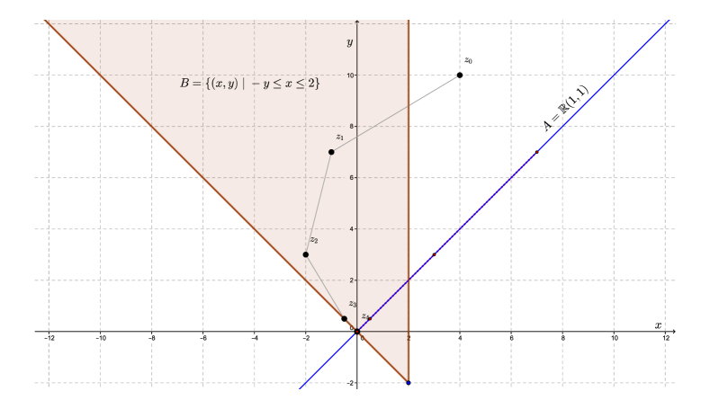
Figure 1: The DRA for the case when $B$ is not a Cartesian product.

4.2 Solving linear equalities with a strict positivity constraint

In this subsection, we assume that

$$X=\mathbb{R}^{N},$$ (87)

and that

$$A=\left\{{x\in X}~{}\big{|}~{}{Lx=a}\right\}\;\;\text{and}\;\;B=\mathbb{R}^{N}_{+},$$ (88)

where $L\in\mathbb{R}^{M\times N}$ and $a\in\mathbb{R}^{M}$. Note that the set $A\cap B$ is polyhedral yet $A\cap B$ has empty interior (unless $A=X$ which is a case of little interest). Thus, Spingarn’s finite-convergence result is never applicable. However, Theorem 3.7 guarantees finite convergence of the DRA provided that Slater’ condition

$$\mathbb{R}^{N}_{++}\cap L^{-1}a\neq\varnothing$$ (89)

holds. Using [5, Lemma 4.1], we obtain

$$P_{A}\colon X\to X\colon x\mapsto x-L^{\dagger}(Lx-a),$$ (90)

where $L^{\dagger}$ denotes the Moore-Penrose inverse of $L$. We also have (see, e.g., [2, Example 6.28])

$$P_{B}\colon X\to X\colon x=(\xi_{1},\dots,\xi_{N})\mapsto x=(\xi_{1}^{+},\dots,\xi_{N}^{+}),$$ (91)

where $\xi^{+}=\max\{\xi,0\}$ for every $\xi\in\mathbb{R}$. This implies $R_{A}\colon X\to X\colon x\mapsto x-2L^{\dagger}(Lx-a)$ and $R_{B}\colon X\to X\colon x=(\xi_{1},\dots,\xi_{N})\mapsto(|\xi_{1}|,\ldots,|\xi_{N}|)$. We will compare three algorithms, all of which generate a governing sequence with starting point $z_{0}\in X$ via

$$(\forall{n\in{\mathbb{N}}})\quad z_{n+1}=Tz_{n}.$$ (92)

The DRA uses, of course,

$$T=\operatorname{Id}-P_{A}+P_{B}R_{A}.$$ (93)

The second method is the classical method of alternating projections (MAP) where

$$T=P_{A}P_{B};$$ (94)

while the third method of reflection-projection (MRP) employs

$$T=P_{A}R_{B}.$$ (95)

We now illustrate the performance of these three algorithms numerically. For the remainder of this section, we assume that that $X=\mathbb{R}^{2}$, that $A=\left\{{(x,y)\in\mathbb{R}^{2}}~{}\big{|}~{}{x+5y=6}\right\}$, and that $B=\mathbb{R}_{+}^{2}$. Then $A$ and $B$ satisfy (89), and the sequence (93) generated by the DRA thus converges finitely to a point in $A\cap B$ regardless of the starting point. See Figure 2 for an illustration, created with GeoGebra [13].

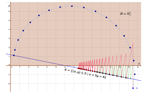
Figure 2: The orbits of DRA (blue), MAP (green) and MRP (red).

Note that the shadow sequence $(P_{A}z_{n})_{n\in{\mathbb{N}}}$ for the DRA finds a point in $A\cap B$ even before a fixed point is reached. For each starting point $z_{0}\in[-100,100]^{2}\subseteq\mathbb{R}^{2}$, we perform the DRA until $z_{n+1}=z_{n}$, and run the MAP and the MRP until $d_{B}(z_{n})=\max\{d_{A}(z_{n}),d_{B}(z_{n})\}<\varepsilon$, where we set the tolerance $\varepsilon=10^{-4}$. Figure 3 compares the number of iterations needed to stop each algorithm. Note that even though we put the DRA at an “unfair disadvantage” (it must find a true fixed point while the MAP and the MRP will stop with $\varepsilon$-feasible solutions), it does extremely well. In Figure 4, we level the playing field and compare the distance from $P_{A}z_{n}$ (for the DRA) or from $z_{n}$ (for the MAP and the MRP) to $B$, where $n\in\{5,10\}$.

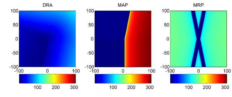
Figure 3: Number of iterations needed to get the solution of DRA, MAP and MRP.

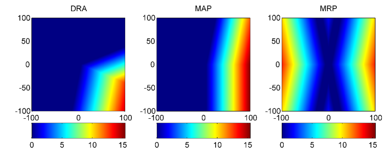
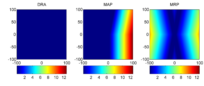
Figure 4: The distance from the monitored iterate to $B$ after $5$ steps (top) and $10$ steps (bottom).

Now we look at the process of reaching a solution for each algorithm. For the DRA, we monitor the shadow sequence $(P_{A}z_{n})_{n\in{\mathbb{N}}}$ and for the MAP and the MRP, we monitor $(z_{n})_{n\in{\mathbb{N}}}$. Note all three monitored sequences lie in $A$, and we thus are concerned about the distance to $B$. Our stopping criterion is that

$$d_{B}(P_{A}z_{n})<\varepsilon$$ (96)

for the DRA, and

$$d_{B}(z_{n})<\varepsilon$$ (97)

for the MAP and the MRP. From top to bottom in Figure 5, we check how many iterates are required to get to tolerance $\varepsilon=10^{-m}$, where $m\in\{2,4\}$, respectively.

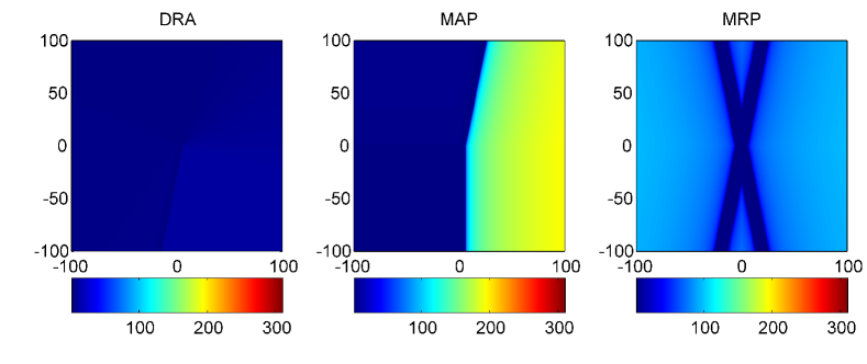
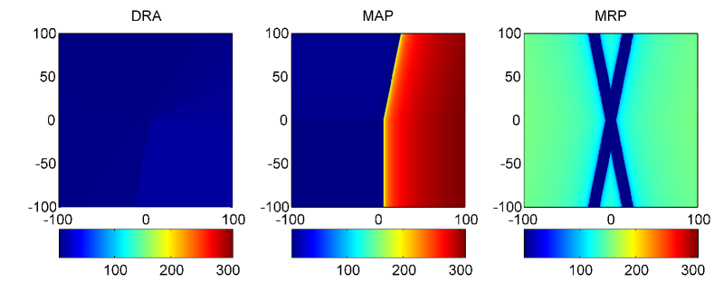
Figure 5: Number of iterations needed to get the tolerance $10^{-2}$ (top) and $10^{-4}$ (bottom) of DRA, MAP and MRP.

Computations were performed with MATLAB R2013b [18]. These experiments illustrate the superior convergence behaviour of the DRA compared to the MAP and the MRP.

5 The hyperplanar-epigraphical case with Slater’s condition

In this section we assume that

$$f\colon X\to\mathbb{R}$$ is convex and continuous. (98a)

We will work in $$X\times\mathbb{R}$$, where we set

$$A:=X\times\{0\}$$ (98b)

and

$$B:=\operatorname{epi}f:=\left\{{(x,\rho)\in X\times\mathbb{R}}~{}\big{|}~{}{f(x)\leq\rho}\right\}.$$ (98c)

Then

$$P_{A}\colon X\times\mathbb{R}\to X\times\mathbb{R}\colon(x,\rho)\mapsto(x,0),$$ (99)

and the projection onto $B$ is described in the following result.

Lemma 5.1

Let $(x,\rho)\in(X\times\mathbb{R})\smallsetminus B$. Then there exists $p\in X$ such that $P_{B}(x,\rho)=(p,f(p))$,

$$x\in p+\big{(}f(p)-\rho\big{)}\partial f(p)\;\text{and}\;\rho<f(p)\leq f(x)$$ (100)

and

$$(\forall y\in X)\quad\left\langle{y-p},{x-p}\right\rangle\leq\big{(}f(y)-f(p)\big{)}\big{(}f(p)-\rho\big{)}.$$ (101)

Moreover, the following hold:

1. If $u$ is a minimizer of $f$, then $\left\langle{u-p},{x-p}\right\rangle\leq 0$.

2. If $x$ is a minimizer of $f$, then $p=x$.

3. If $x$ is not a minimizer of $f$, then $f(p)<f(x)$.

Proof.

According to [2, Proposition 28.28], there exists $(p,p^{*})\in\operatorname{gra}\partial f$ such that $P_{B}(x,\rho)=(p,f(p))$ and $x=p+(f(p)-\rho)p^{*}$. Next, [2, Propositions 9.18] implies that $\rho<f(p)$ and (101). The subgradient inequality gives

$$f(x)-f(p)\geq\left\langle{p^{*}},{x-p}\right\rangle=\left\langle{p^{*}},{(f(p)-\rho)p^{*}}\right\rangle=(f(p)-\rho)\|p^{*}\|^{2}\geq 0.$$ (102)

Hence $f(p)\leq f(x)$, and this completes the proof of (100),

(i): It follows from (101) that $\left\langle{u-p},{x-p}\right\rangle\leq(f(u)-f(p))(f(p)-\rho)$. Since $f(p)-\rho>0$ and $f(u)\leq f(p)$, we have $\left\langle{u-p},{x-p}\right\rangle\leq 0$.

(ii): Apply (i) with $u=x$.

(iii): By (100), $\rho<f(p)\leq f(x)$. We show the contrapositive and thus assume that $f(p)=f(x)$. Since $f(p)-\rho>0$, (102) yields $p^{*}=0$, and so $0\in\partial f(p)$. It follows that $p$ is a minimizer of $f$, and therefore $x$ also minimizes $f$. ∎

Remark 5.2

When $X=\mathbb{R}$ and $u$ is a minimizer of $f$, then $(u-p)(x-p)\leq 0$ by Lemma 5.1(i). Therefore, $p$ lies between $x$ and $u$ (see also [4, Corollary 4.2]).

Define the DRA operator by

$$T:=\operatorname{Id}-P_{A}+P_{B}R_{A}.$$ (103)

It will be convenient to abbreviate

$$B^{\prime}:=R_{A}(B)=\left\{{(x,\rho)\in X\times\mathbb{R}}~{}\big{|}~{}{\rho\leq-f(x)}\right\}$$ (104)

and to analyze the effect of performing one DRA step in the following result.

Corollary 5.3 (one DRA step)

Let $z=(x,\rho)\in X\times\mathbb{R}$, and set $z_{+}:=(x_{+},\rho_{+})=T(x,\rho)$. Then the following hold:

1. Suppose that $z\in B^{\prime}$. Then $z_{+}=(x,0)\in A$. Moreover, either ($f(x)\leq 0$ and $z_{+}\in A\cap B$) or ($f(x)>0$ and $z_{+}\not\in B\cup B^{\prime}$).

2. Suppose that $z\not\in B^{\prime}$. Then there exists $x_{+}^{*}\in\partial f(x_{+})$ such that

   $$x_{+}=x-\rho_{+}x_{+}^{*},\;f(x_{+})\leq f(x),\;\text{and}\;\rho_{+}=\rho+f(x_{+})>0.$$ (105)

   Moreover, either ($\rho\geq 0$ and $z_{+}\in B$) or ($\rho<0$, $z_{+}\not\in B\cup B^{\prime}$ and $Tz_{+}\in B$).

3. Suppose that $z\in B\cap B^{\prime}$. Then $z_{+}\in A\cap B$.

4. Suppose that $z\in B\smallsetminus B^{\prime}$. Then $z_{+}\in B$.

Proof.

(i): We have $P_{A}z=(x,0)$ and $R_{A}z=(x,-\rho)\in B$. Thus $P_{B}R_{A}z=P_{B}(x,-\rho)=(x,-\rho)$, which gives

$$z_{+}=(\operatorname{Id}-P_{A}+P_{B}R_{A})z=(x,\rho)-(x,0)+(x,-\rho)=(x,0)\in A.$$ (106)

If $f(x)\leq 0$, then $z_{+}=(x,0)\in B$, and hence $z_{+}\in A\cap B$. Otherwise, $f(x)>0$ which implies $-f(x)<0$ and further $z_{+}=(x,0)\not\in B\cup B^{\prime}$.

(ii): We have $R_{A}z=(x,-\rho)\not\in B$, and by (100), $P_{B}(x,-\rho)=(p,f(p))$, where

$$p=x-(\rho+f(p))p^{*}\text{ for some }p^{*}\in\partial f(p),\quad\text{and}\quad-\rho<f(p)\leq f(x).$$ (107)

We obtain

$$z_{+}=(x_{+},\rho_{+})=(\operatorname{Id}-P_{A}+P_{B}R_{A})z=(x,\rho)-(x,0)+(p,f(p))=(p,\rho+f(p)),$$ (108)

which gives $x_{+}=p$ and $\rho_{+}=\rho+f(p)>0$, so (105) holds. If $\rho\geq 0$, then $\rho_{+}=\rho+f(x_{+})\geq f(x_{+})$, and thus $z_{+}\in B$. Otherwise, $\rho<0$, so $\rho_{+}<f(x_{+})$ and also $f(x_{+})>-\rho>0$. Hence $\rho_{+}>0>-f(x_{+})$, which implies $z_{+}\not\in B\cup B^{\prime}$, and then $Tz_{+}\in B$ because $\rho_{+}>0$ and the previous case applies.

(iii): We have $f(x)\leq\rho\leq-f(x)$, and so $f(x)\leq 0$. Now apply (i).

(iv): We have $\rho\geq f(x)$ and $\rho>-f(x)$. Then $\rho\geq|f(x)|\geq 0$, and (ii) gives $z_{+}\in B$. ∎

Theorem 5.4

Suppose that $\inf_{X}f<0$, and, given a starting point $z_{0}=(x_{0},\rho_{0})\in X\times\mathbb{R}$, generate the DRA sequence $(z_{n})_{n\in{\mathbb{N}}}$ by

$$(\forall{n\in{\mathbb{N}}})\quad z_{n+1}=(x_{n+1},\rho_{n+1})=Tz_{n}.$$ (109)

Then $(z_{n})_{n\in{\mathbb{N}}}$ converges finitely to a point $z\in A\cap B$.

Proof.

In view of Corollary 5.3(i)&(iii), we can and do assume that $z_{0}\in B\smallsetminus B^{\prime}$, where $B^{\prime}$ was defined in (104). It follows then from Corollary 5.3(iii)&(iv), that $(z_{n})_{n\in{\mathbb{N}}}$ lies in $B$.

Case 1: $(\exists n\in\mathbb{N})$ $z_{n}\in B\cap B^{\prime}$.
By Corollary 5.3(iii), $z_{n+1}\in A\cap B$ and we are done.

Case 2: $(\forall{n\in{\mathbb{N}}})$ $z_{n}\in B\smallsetminus B^{\prime}$.
By Corollary 5.3(ii),

$$(\forall{n\in{\mathbb{N}}})\quad f(x_{n+1})\leq f(x_{n})\;\;\text{and}\;\;\rho_{n+1}=\rho_{n}+f(x_{n+1})>0.$$ (110)

Next, it follows from [22, Lemma 7.3] that $\operatorname{int}B=\left\{{(x,\rho)\in X\times\mathbb{R}}~{}\big{|}~{}{f(x)<\rho}\right\}$. Because $\inf_{X}f<0$, we obtain $A\cap\operatorname{int}B\neq\varnothing$, which, due to Lemma 3.2(i) yields $z_{n}\to z=(x,\rho)\in A\cap B$. Since $z\in A$, we must have $\rho=0$. If $(\forall{n\in{\mathbb{N}}})$ $f(x_{n+1})\geq 0$, then, by (110), $0<\rho_{1}\leq\rho_{2}\leq\cdots\leq\rho_{n}\to\rho=0$ which is absurd. Therefore,

$$(\exists\,n_{0}\in\mathbb{N})\quad f(x_{n_{0}+1})<0.$$ (111)

In view of (110), we see that $(\forall n\geq n_{0}+1)$ $\rho_{n}\leq\rho_{n_{0}}+(n-n_{0})f(x_{n_{0}+1})$. Since $f(x_{n_{0}+1})<0$, there exists $n_{1}\in\mathbb{N}$, $n_{1}\geq n_{0}+1$ such that

$$\rho_{n_{0}}+(n_{1}-n_{0})f(x_{n_{0}+1})\leq-f(x_{n_{0}+1}).$$ (112)

Noting that $f(x_{n_{1}})\leq f(x_{n_{0}+1})$, we then obtain

$$\rho_{n_{1}}\leq\rho_{n_{0}}+(n_{1}-n_{0})f(x_{n_{0}+1})\leq-f(x_{n_{0}+1})\leq-f(x_{n_{1}}).$$ (113)

Hence $z_{n_{1}}\in B^{\prime}$, which contradicts the assumption of Case 2. Therefore, Case 2 never occurs and the proof is complete. ∎

We conclude by illustrating that finite convergence may be deduced from Theorem 5.4 but not necessarily from the finite convergence conditions of Section 2.6.

Example 5.5

Suppose that $X=\mathbb{R}$, that $A=\mathbb{R}\times\{0\}$, and that $B=\operatorname{epi}f$, where $f\colon\mathbb{R}\to\mathbb{R}\colon x\mapsto x^{2}-1$. Let $(\forall\varepsilon\in\mathbb{R}_{++})$ $z_{\varepsilon}=(1+\varepsilon,-\varepsilon)$. Then $(\forall\varepsilon\in\mathbb{R}_{++})$ $Tz_{\varepsilon}\notin\operatorname{Fix}T=[-1,1]\times\{0\}$, and $z_{\varepsilon}-Tz_{\varepsilon}\to 0$ as $\varepsilon\to 0^{+}$. Consequently, Luque’s condition (41) fails.

Proof.

Let $\varepsilon\in\mathbb{R}_{++}$. Then $-f(1+\varepsilon)=-2\varepsilon-\varepsilon^{2}<-\varepsilon$, and so $z_{\varepsilon}=(1+\varepsilon,-\varepsilon)\notin B^{\prime}$. By Corollary 5.3(ii), there exists $x_{\varepsilon}\in\mathbb{R}$ such that

$$Tz_{\varepsilon}=(x_{\varepsilon},-\varepsilon+f(x_{\varepsilon})),\quad x_{\varepsilon}=1+\varepsilon-(-\varepsilon+f(x_{\varepsilon}))2x_{\varepsilon},\quad\text{and}\quad-\varepsilon+f(x_{\varepsilon})>0.$$ (114)

The last inequality shows that $Tz_{\varepsilon}\notin\operatorname{Fix}T=[-1,1]\times\{0\}$. It follows from the expression of $x_{\varepsilon}$ that

$$2x_{\varepsilon}^{3}-(1+2\varepsilon)x_{\varepsilon}-1-\varepsilon=0.$$ (115)

Note that $(x_{\varepsilon},f(x_{\varepsilon}))+(0,-\varepsilon)=Tz_{\varepsilon}=z_{\varepsilon}-P_{A}z_{\varepsilon}+P_{B}R_{A}z_{\varepsilon}=(1+\varepsilon,-\varepsilon)-(1+\varepsilon,0)+P_{B}(1+\varepsilon,\varepsilon)=P_{B}(1+\varepsilon,\varepsilon)+(0,-\varepsilon)$ and hence $(x_{\varepsilon},f(x_{\varepsilon}))=P_{B}(1+\varepsilon,\varepsilon)$. Remark 5.2 gives $0\leq x_{\varepsilon}\leq 1+\varepsilon$. If $0\leq x_{\varepsilon}\leq 1$, then (115) yields $0\leq 2x_{\varepsilon}-(1+2\varepsilon)x_{\varepsilon}-1-\varepsilon=(x_{\varepsilon}-1)-2\varepsilon x_{\varepsilon}-\varepsilon<0$, which is absurd. Thus $1<x_{\varepsilon}\leq 1+\varepsilon$. Now as $\varepsilon\to 0^{+}$, we have $x_{\varepsilon}\to 1$, $f(x_{\varepsilon})\to f(1)=0$, and at the same time, $z_{\varepsilon}-Tz_{\varepsilon}=(1+\varepsilon-x_{\varepsilon},-f(x_{\varepsilon}))\to 0$. ∎

Acknowledgments

HHB was partially supported by the Natural Sciences and Engineering Research Council of Canada and by the Canada Research Chair Program. MND was partially supported by an NSERC accelerator grant of HHB.

References

- [1] H.H. Bauschke, J.Y. Bello Cruz, T.T.A. Nghia, H.M. Phan, and X. Wang, The rate of linear convergence of the Douglas–Rachford algorithm for subspaces is the cosine of the Friedrichs angle, Journal of Approximation Theory 185 (2014), 63–79.
- [2] H.H. Bauschke and P.L. Combettes, Convex Analysis and Monotone Operator Theory in Hilbert Spaces, Springer, 2011.
- [3] H.H. Bauschke, P.L. Combettes, and D.R. Luke, Finding best approximation pairs relative to two closed convex sets in Hilbert spaces, Journal of Approximation Theory 127 (2004), 178–192.
- [4] H.H. Bauschke, M.N. Dao, D. Noll, and H.M. Phan, Proximal point algorithm, Douglas–Rachford algorithm and alternating projections: a case study, Journal of Convex Analysis, to appear.
- [5] H.H. Bauschke and S.G. Kruk, Reflection–projection method for convex feasibility problems with an obtuse cone, Journal of Optimization Theory and Applications 120 (2004), 503–531.
- [6] H.H. Bauschke, D. Noll, and H.M. Phan, Linear and strong convergence of algorithms involving averaged nonexpansive operators, Journal of Mathematical Analysis and Applications 421 (2015), 1–20.
- [7] J.M. Borwein and W.B. Moors, Stability of closedness of convex cones under linear mappings, Journal of Convex Analysis 16 (2009), 699–705.
- [8] A. Cegielski, Iterative Methods for Fixed Point Problems in Hilbert Spaces, Springer, 2012.
- [9] Y. Censor and S.A. Zenios, Parallel Optimization, Oxford University Press, 1997.
- [10] P.L. Combettes, Iterative construction of the resolvent of a sum of maximal monotone operators, Journal of Convex Analysis 16 (2009), 727–748.
- [11] J. Douglas and H.H. Rachford, On the numerical solution of heat conduction problems in two and three space variables, Transactions of the AMS 82 (1956), 421–439.
- [12] J. Eckstein and D.P. Bertsekas, On the Douglas–Rachford splitting method and the proximal point algorithm for maximal monotone operators, Mathematical Programming 55 (1992), 293–318.
- [13] GeoGebra software, http://www.geogebra.org
- [14] R. Hesse and D.R. Luke, Nonconvex notions of regularity and convergence of fundamental algorithms for feasibility problems, SIAM Journal on Optimization 23 (2013), 2397–2419.
- [15] J. Lawrence and J.E. Spingarn, On fixed points of nonexpansive piecewise isometric mappings, Proceedings of the London Mathematical Society. Third Series 55 (1987), 605–624.
- [16] P.-L. Lions and B. Mercier, Splitting algorithms for the sum of two nonlinear operators, SIAM Journal on Numerical Analysis 16 (1979), 964–979.
- [17] F.J. Luque, Asymptotic convergence analysis of the proximal point algorithm, SIAM Journal on Control and Optimization 22 (1984), 277–293.
- [18] MATLAB software, http://www.mathworks.com/products/matlab/
- [19] P. Mahey, S. Oualibouch, and P.D. Tao, Proximal decomposition on the graph of a maximal monotone operator, SIAM Journal on Optimization 5 (1995), 454–466.
- [20] B.S. Mordukhovich and N.M. Nam, An Easy Path to Convex Analysis and Applications, Morgan & Claypool Publishers, 2014.
- [21] H.M. Phan, Linear convergence of the Douglas–Rachford method for two closed sets, preprint 2014, http://arxiv.org/abs/1401.6509
- [22] R.T. Rockafellar, Convex Analysis, Princeton University Press, 1970.
- [23] R.T. Rockafellar, Monotone operators and the proximal point algorithm, SIAM Journal on Control and Optimization 14(5) (1976), 877–898.
- [24] R.T. Rockafellar and R.J.-B. Wets, Variational Analysis, Springer-Verlag, 1998.
- [25] J.E. Spingarn, Partial inverse of a monotone operator, Applied Mathematics and Optimization 10 (1983), 247–265.
- [26] J.E. Spingarn, A primal-dual projection method for solving systems of linear inequalities, Linear Algebra and its Application 65 (1985), 45–62.