Modeling Recovery Curves With Application to Prostatectomy

Abstract

In many clinical settings, a patient outcome takes the form of a scalar time series with a recovery curve shape, which is characterized by a sharp drop due to a disruptive event (e.g., surgery) and subsequent monotonic smooth rise towards an asymptotic level not exceeding the pre-event value. We propose a Bayesian model that predicts recovery curves based on information available before the disruptive event. A recovery curve of interest is the quantified sexual function of prostate cancer patients after prostatectomy surgery. We illustrate the utility of our model as a pre-treatment medical decision aid, producing personalized predictions that are both interpretable and accurate. We uncover covariate relationships that agree with and supplement that in existing medical literature.

1 Introduction

In the medical community, there is a pressing need for personalized predictions of how a disruptive event, such as a treatment or disease, will impact particular bodily function levels. Of particular interest is the extent to which the function is initially perturbed by the event and the ensuing pattern of recovery. In many contexts, such as mental acuity following a stroke or sexual function following prostatectomy, the post-event trajectory generally exhibits what we call a recovery curve shape, characterized by an initial instantaneous drop followed by a monotonic rise towards an asymptotic level not exceeding the original function level. Here, we propose a Bayesian model that can be used to predict a patient’s expected recovery curve, given information about the patient that is available before the event.

This paper presents a decision aid for patients considering a medical treatment who want to know what adverse side effect the treatment would have on a particular bodily function. In particular, our model will be used to display to the patient a distribution over post-treatment function trajectories, conveying the uncertainty in predictions that should be considered in decision-making. We assume that the function level lies in some closed interval, the pre-treatment function level is known, and the adverse effect of the event on the function is a priori known by the medical community to be immediate, but wearing off over time.

If a model is to be widely adopted as a medical decision aid, it is not enough for it to merely produce predictions that are accurate; it must also be interpretable: it must give predictions that a healthcare provider or patient can readily understand. This is crucial in a clinical setting not only because of time constraints, but also because each additional point of confusion regarding the predictions decreases the flow of information to the patient and thus their trust in it. Any model, including ours, should be used only if it fits the data, and standard model checking should be performed. However, aggregate model fit and predictive accuracy are not sufficient; when a tool causes more questions than it answers, it will be less likely to be used.

In the applications we consider, we will predict time series that are expected to be recovery curves. These recovery curves occur in practice in situations where a medical procedure may cause a temporary inhibition or detriment in a patient, but will not improve the patient’s condition over a baseline value. In our case, we examine sexual function in patients with prostate cancer who are considering a prostatectomy. Though a prostatectomy will likely decrease sexual function in some patients, it will not improve a patient’s sexual function above the baseline.

We restrict the space of possible outputs to our model, therefore, to only include predictions that are recovery curves. In other words, our model outputs a distribution of post-event trajectories each of which is guaranteed to be a recovery curve, so that the function level drops instantaneously downwards at event time, and rises smoothly to approach an asymptotic level lying between the pre-treatment value and value immediately following treatment (we will use the words “level” and “value” interchangeably). Furthermore, our model encourages the posterior predictive distribution over trajectories to have a well defined mode, so that the distribution of curves, when plotted, can be visually easily interpreted as a single maximum a posteriori prediction along with the uncertainty in that single prediction. Thus, not only do the predictions match prior expections, but they are also simple, defined by a small set of salient features (i.e. initial drop, recovery rate, and range of uncertainty), not containing extraneous artifacts that slightly increase accuracy but greatly reduce interpretability.

We use our method to create a decision aid for prostate cancer patients who are considering a prostatectomy, predicting their sexual function trajectory, should they undergo a prostatectomy. We fit our model using data from a study that tracked the quantified sexual function level, expressed as a number between 0 and 1, of 237 patients both before radical prostatectomy surgery and at a common set of timepoints in the 4 years immediately following surgery. These numerical measures of sexual function were obtained by administering the Prostate Cancer Index, which is a multiple choice questionaire that first evaluates patient function and bother following prostate cancer treatment, and then converts the answers to a numerical score. Note that while our target population is patients merely considering a prostatectomy (and satisfies two properties listed shortly), our dataset only contains data from patients who actually did undergo a prostatectomy.

Prostate cancer will affect 1 out of 6 men, and low stage patients usually have several viable treatment options, each with different side effects. Radical prostatectomy is known to adversely affect sexual function. Thus, for patients considering prostatectomy, it is important to forecast the pattern of sexual function level should they undergo one. Past studies (Potosky and others, 2004) and our dataset indicate that sexual function trajectories after prostatectomy follow a recovery curve (at least up to 5 years post-treatment), suggesting our model may fit such trajectories well.

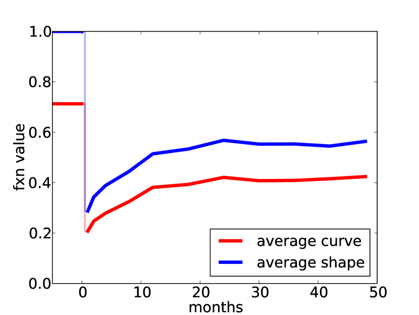
(a) The average function value and scaled function value over the prostatectomy dataset exhibit a recovery curve shape.

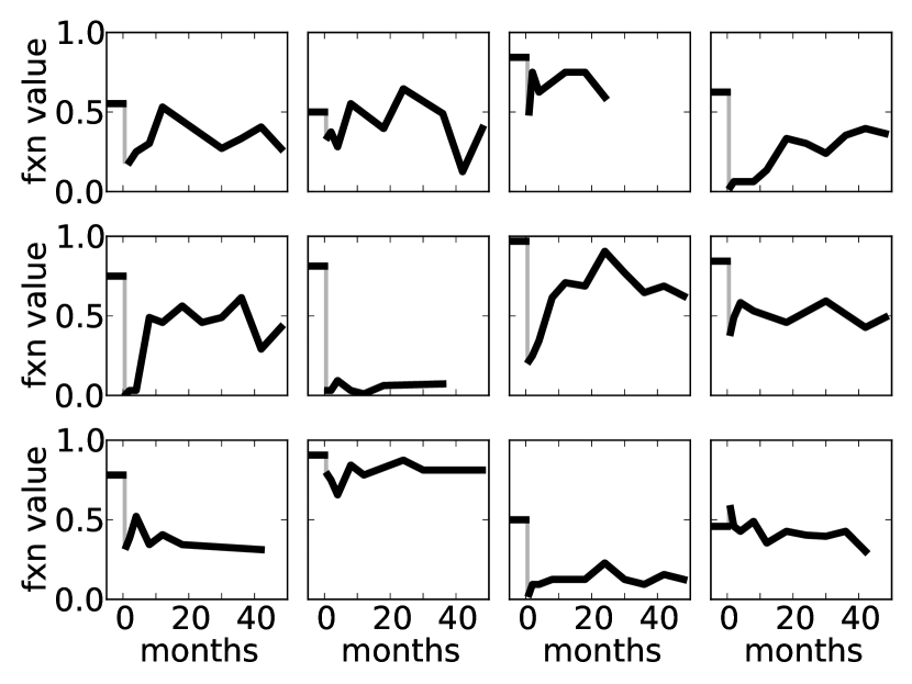
(b) Raw data of 12 randomly chosen patients who passed the filters as described in Section 6.1.

Figure 1: Sexual function trajectory (fxn value) following prostatectomy.

To illustrate, in Figure 1(a) we show the dataset-wide averages, for each timepoint, of sexual function level (fxn level), as well as dataset-wide averages, for each timepoint, of the patients’ sexual function values scaled by their respective value immediately before prostatectomy. We also show in Figure 1(b) the unscaled sexual function level time series of 12 randomly selected patients, which includes their unscaled sexual function level both post-treatment and right before treatment. We hypothesize that the function levels reported by individual patients are noisy versions of a latent smooth “true” function level. In this context, we use our method to study whether there are patient covariates that correlate with post-surgery sexual function trajectory.

The remainder of the paper is organized as follows. In Section 2 we contextualize our approach by describing related work. Then, we formally define the recovery curve shape in Section 3 and present the specifics of our model in Section 4. We demonstrate that the model performs well in simulation studies in Section 5 and then using the aforementioned prostatecomy data in Section 6.

2 Related Work

Past work on personalized prediction of sexual function following prostate cancer treatment has attempted to predict a post-operative binary outcome, typically whether one is able to achieve an erection sufficient for sex at some single timepoint following treatment (Regan and others, 2011; Descazeaud and others, 2006; Eastham and others, 2008; Ayyathurai and others, 2008), or the change in (Sanda and others, 2008) or absolute level (Talcott and others, 2003) of some continuous measure of sexual function such as the IIEF-5 score. Such models incorporated patient covariates in linear regression models for continuous outcomes, and logistic regression models for binary outcomes even though sexual function is not a binary outcome (Briganti and others, 2011). Another deficiency of logistic and linear regression is that they are not suitable for modeling longitudinal outcomes, whereas a patient would want to know their entire post-treatment function trajectory. The only longitudinal model in the literature uses linear regression to relate the change in function level between two fixed timepoints post-treatment (Potosky and others, 2004).

Functional data analysis (Ramsay and Silverman, 2002; Denison and others, 1998) and growth curve modeling (Jung and Wickrama, 2008) are rich areas of past study, but existing models from those fields do not guarantee that the predicted time series possesses a recovery curve shape, that it drops following the event and then monotonically approaches an asymptotic level no higher than the pre-event value. Parametric functions mentioned in Rogosa and Willett (1985) resemble the functional form we assume of recovery curves. However, they are modeling growth, not recovery after some disruptive event, and assume the initial level of the growth curve to be known, whereas we are trying to predict the entire post-treatment trajectory, which includes the initial post-treatment value. Furthermore, they do not place an upper bound on the asymptotic level of the predicted function. Isotonic regression models (Shively and others, 2009; Mammen, 1991; Neelon and Dunson, 2004; Cai and Dunson, 2007), enforce the predicted functions to be monotonic, but do not naturally output recovery curves as predictions.

Other statistical models have also been applied in contexts where the predicted time series is expected to exhibit a recovery curve shape. For example, in a medical context, growth curve techniques have been used to model recovery of a bodily function following a disruptive event. Warschausky and others (2001) model recovery of FIM-measured function following spinal surgery as being the sum of a linear and a plateauing function. Although the FIM-score must lie within a bounded interval, they do not guarantee that the predicted scores lie within that interval. Rolfe and others (2011) model verbal function following chemotherapy using a Bayesian latent basis model, but the model lacks incorporation of patient-correlates, and is instead specialized to infer average recovery at only two fixed timepoints. Tilling and others (2001) model a measure of quality of life - the Barthel Index - following stroke using a multilevel model where both patient-specific and time-specific contributions are modeled as a linear combination of a fractional polynomial basis. In all these models, the predicted time series is expected to possess a recovery curve shape, but there is no explicit constraint built into the models to ensure that the predicted trajectory actually does possesses a recovery curve shape.

Two past works suggest that a model of sexual function following prostatectomy needs a significant amount of interpretability-promoting features if it is to be used in practice. One work involved eliciting and incorporating the preferences of patients, providers, and design experts via a 3-step human-centered design process to design such dashboards (Hartzler and others, 2015). The second work measured patients’ abilities to understand 3 different visual displays communicating the same information - bar charts, line graph, and table, and examined how a patient’s understanding of those 3 displays related to their demographics (i.e. education level, race) and graphical and numerical literacy as measured through the REALM and SNS questionaires, two standard medical instruments (Nayak and others, 2015). One takeway from these works is just how much detail, care, and user feedback goes into designing visual dashboards and studying the impact of seemingly small changes to them. One example of a small design decision significant enough to warrant study was, in a pictogram used to communicate well-being, whether a sunny weather/cloudy weather icon should be used in place of a smiling/frowning face to represent well being. These meticulous studies reflect the sensitivity of patient comprehension to dashboard features, and suggest each additional feature improving the interpretability of our model can greatly improve patient comprehension and thus clinical applicability. A second takeaway from these works is that some patients prefer extremely simple dashboards. For example, some patients felt that putting confidence intervals on personalized predictions was too confusing, preferring a point prediction instead. This preference bolsters the case for our unimodality requirement - given that some patients do not even want to see uncertainty in predictions, were we to display them, we should do so in the simplest manner possible. In any case, this second takeaway suggests many interpretability-promoting features may be necessary for any clinical applicability at all.

3 Recovery Curves

3.1 Recovery Curve Definition

A recovery curve is a function $f(t)$ defined on $\mathbb{R^{+}}$. We will always define $f(t)$ piecewise as

$$f(t)=\begin{cases}\hfill S\hfill&\text{ for $t=0$},\\ \hfill f^{+}(t)\hfill&\text{ for $t>0$,}\\ \end{cases}$$ (3.1)

which is interpreted as the disruptive event occuring right after time 0, so that $S$ is the (known) pre-treatment function value, and $f^{+}(t)$ is the post-treatment trajectory. A recovery curve will satisfy the following:

$$(f^{+})^{\prime} >0\text{ for t $>$ 0},$$ (3.2)

$$f^{+}(t) \leq S\text{ for t $>$ 0, }$$ (3.3)

$$f^{+}(t) \geq 0\text{ for t $>$ 0, }$$ (3.4)

$$S \in[0,1].$$ (3.5)

3.2 Parameterizing Recovery Curves

We parameterize $f(t)$ scaled to the pre-treatment function value, instead of $f(t)$ itself, assuming:

$$f^{+}(t;S,\theta)=Sg(t;\theta).$$ (3.6)

Thus, the actual post-event trajectory is the shape of the post-event trajectory, $g(t;\theta)$, scaled to the pre-event function level. We choose this parameterization because in order to satisfy requirements of Equations 3.3 and 3.4, we just need to ensure that $g(t;\theta)\in(0,1)$ for $t>0$. In this work we will refer to the scaled post-event trajectory, denoted $g(t;\theta)$, as a recovery shape, and use the term scaled function value to refer to a patient’s function value normalized by their pre-treatment value; a patient’s recovery shape is a time series over their scaled function values.

We parameterize recovery shape $g(t;\theta)$ with 3 parameters: $A$, the asymptotic drop in scaled function level after surgery, $B$, the initial drop in scaled function value in excess of the asymptotic drop, and $C$, the rate of recovery of the scaled function value.

$$f(t;S,A,B,C) =Sg(t;A,B,C),\ \text{where}$$ (3.7)

$$g(t;A,B,C) =S\left(1-A-B(1-A)\exp\left({}^{-}\frac{t}{C}\right)\right),$$ (3.8)

$$A\in[0,1],B\in[0,1],C\geq 0.$$ (3.9)

$f(t;S,A,B,C)$ is a recovery curve if the constraints in Equations 3.2 to 3.5 are satisfied, and we respect those constraints in our model.

4 Model

The previous section formalized the definition or a recovery curve. To fit the curves to data and make meaningful predictions for patients, however, we need both the shape of the curve and a framework for inference. In this section, we describe a Bayesian approach to fitting recovery curves. We first describe the structure of the statistical model, then we note the properties of the model that make it well-suited for situations where we expect recovery curve trajectories.

Throughout the section, we refer to the $i\text{-}th$ patient’s covariate vector as $X_{i}\in\mathbb{R}^{K}$ where $K$ is the number of features per patient, and their observed function value at time $t$ by $y_{i}(t)$. Here, $y_{i}(t)$ is considered a noisy measurement of their “underlying” function value at time $t$, $f(t;S_{i},A_{i},B_{i},C_{i})$, where $f(\cdot;S_{i},A_{i},B_{i},C_{i})$ is the parameterization of post-treatment function value described in Section 3.2. The noise in $y_{i}(t)$ could arise from a number of sources, including short-term fluctuations in patients’ experiences or difficulty in recalling function between time periods. The “underlying” function value, $f(t;S_{i},A_{i},B_{i},C_{i})$, is a function of the patient’s pre-treatment function value $S_{i}$ and patient-specific random parameters $A_{i},B_{i},C_{i}$. To simplify notation, we abbreviate the latent function value as $f_{i}(t)$. When making a prediction for a new patient, we assume $S_{i}$ is known based on the patient’s experience before the procedure. In the Supplementary Materials, we study the robustness of our model to measurement error in $S_{i}$.

4.1 Model Components

As previously mentioned, we perform inference on recovery curves using a hierarchical Bayesian model. The Bayesian paradigm facilitates sharing information across similar, but not identical patients. This information sharing is critical in our context as data on outcomes after radical prostatectomy are very difficult to collect and rare. The remainder of this subsection provides a detailed description of the model.

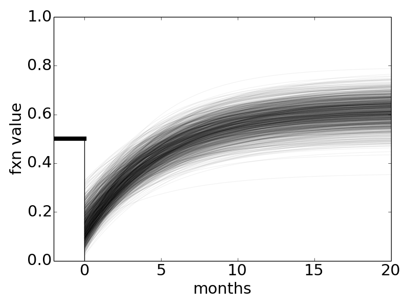
(a) This predictive distribution is unrealistic because some of the time series are not recovery curves, as their post-treatment function value exceeds that pre-treatment.

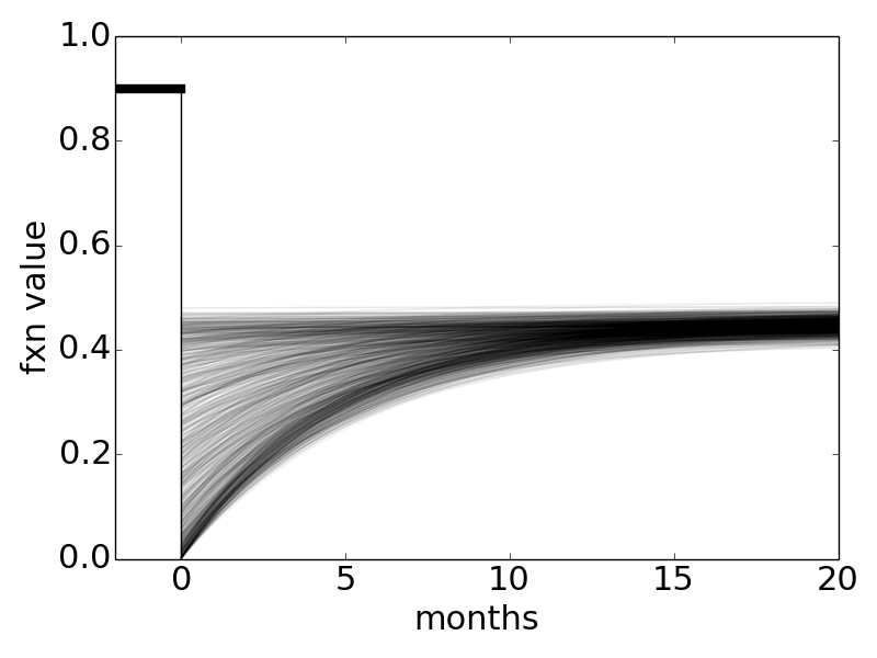
(b) This predictive distribution is unrealistic because the distribution is not unimodal. One can see this because there are two dark sets of curves, one for each mode of the posterior curve distribution.

Figure 2: Two unrealistic predictive distributions

Recall that our model is designed to be interpretable. In particular, a patient’s posterior over recovery curves firstly should only have support over the space of recovery curves, so that a posterior as in Figure 2(a) is not acceptable, containing support over trajectories whose aymptotic level exceeds that pre-treatment. Secondly, the posterior should be unimodal, so that a posterior as in Figure 2(b) is not acceptable. We encourage the first desiderata by appropriately constraining the support of relevant conditional distributions of the model, and the second by guaranteeing unimodality of those conditional distributions by using specialized distribution parameterizations.

First, recall the observed data $y_{i}(t)$ is a patient’s reported function level at time $t$. We assume the reported function level comes from a likelihood that is a mixture distribution of the form:

$$y_{i}(t)|f_{i}(t),\theta,p,\phi_{M} \sim\theta\operatorname{bernoulli}(p)+(1-\theta)\operatorname{beta}_{m,\phi}(f_{i}(t),\phi_{M}),\ \ \text{with}\ p,\theta,\phi_{M}\in(0,1),X_{i}\in\mathbb{R}^{K}.$$

We use a mixture distribution because patients can and do report values of 0 and 1. In the data presented in Section 6, approximately five percent of patient responses are on the boundary of the unit interval. The mixture distribution, therefore, places finite mass on the 0 and 1 responses, but also allows responses between 0 and 1 to be modeled using a recovery curve.

For values other than 0 and 1, we propose a beta distribution that depends on the patient’s (latent) recovery curve value at time $t$, $f_{i}(t)$. Even notwithstanding the potential for values on the boundary, parameterizing the unit interval in a way that is interpretable is challenging. To encourage unimodality of the $y_{i}(t)$, we would like this beta distribution to always be unimodal. For the typical parameterization of the beta distribution, $\operatorname{beta}_{\alpha,\beta}(\alpha^{\prime},\beta^{\prime})$), the mean ($\alpha^{\prime}/\alpha^{\prime}+\beta^{\prime}$) and mode ($\alpha^{\prime}-1/\alpha^{\prime}+\beta^{\prime}-1$) both depend on both parameters. Further, the distribution is only unimodal if $\alpha$ and $\beta$ are both greater than one. As our goal is to develop a method that is easy to explain to clinicians and patients, we chose to reparameterize the beta distribution in terms of mode $m$ and spread parameter $\phi$. This $\operatorname{beta}_{m,\phi}$ parameterization relates to the typical beta as:

$$\operatorname{beta}_{m,\phi}(m^{\prime},\phi^{\prime})=\operatorname{beta}_{\alpha,\beta}\left(1+\left(\frac{1}{\phi^{\prime}}-1\right)m^{\prime},1+\left(\frac{1}{\phi^{\prime}}-1\right)\left(1-m^{\prime}\right)\right).$$ (4.1)

Critically, our $\operatorname{beta}_{m,\phi}(m^{\prime},\phi^{\prime})$ distribution has mode $m^{\prime}$ and for all $m^{\prime}$, is unimodal if and only if spread parameter $\phi^{\prime}\in(0,1)$. Examples of such distributions and a full description of the steps to reparameterize are in Figure 6 and Section 1 of the Supplementary Materials.

For values not on the boundary, each respondents’ reported function value comes from a beta distribution centered on their true (latent) function value, $f_{i}(t)$, and with spread around that function value determined by parameter $\phi_{M}$. The patient’s latent function value takes the form of a recovery curve described in Section 3. Following the Bayesian paradigm, we specify prior distributions for the parameters of the recovery curve. We expect that patients that are observably similar will have similar recovery trajectories, so we model the parameters of each patient’s recovery curve as a function of observable covariates. Recall that the recovery curve depends on individual specific parameters $A_{i},B_{i}$ and $C_{i}$ controlling the asymptotic decrease in function post treatment, initial drop post treatment, and rate of recovery, respectively. Since $A_{i}$ and $B_{i}$ are scaled to be consistent across patients, they have support on $(0,1)$. The $C_{i}$ parameter is a rate and thus has support on $\mathbb{R}^{+}$. We model each with a generalized linear model of the form:

$$A_{i}|b_{A},\phi_{A};z_{A},X_{i} \sim\operatorname{beta}_{m,\phi}(\operatorname{logistic}(z_{A}+b_{A}^{T}X_{i}),\phi_{A})$$ (4.2)

$$B_{i}|b_{B},\phi_{B};z_{B},X_{i} \sim\operatorname{beta}_{m,\phi}(\operatorname{logistic}(z_{B}+b_{B}^{T}X_{i}),\phi_{B})$$ (4.3)

$$C_{i}|b_{C},\phi_{C};z_{C},X_{i} \sim\operatorname{gamma}_{m,\phi}(\operatorname{exp}(z_{C}+b_{C}^{T}X_{i}),\phi_{C}),\ \text{with}$$ (4.4)

$$b_{A},b_{B},b_{C} \in\mathbb{R}^{K},\ \phi_{A},\phi_{B},\phi_{C}\in(0,1),X_{i}\in\mathbb{R}^{K}.$$ (4.5)

Note that by assuming the recovery curve parameterization of Equation 3.8, we are effectively modeling a patient’s function values scaled by their known pre-treatment value. Justification for this approach is given in Section 5 of the Supplementary Materials.

To promote interpretability by encouraging unimodality of conditional distributions, we again use the alternative parameterization of the beta distribution described above for the likelihood. Each patient’s initial drop in function value ($B_{i}$) is centered at a mode given by the expected drop based on patients with similar observable characteristics but with spread $\phi_{B}$. A similar interpretation applies to the eventual drop, $A_{i}$. To ensure that $C_{i}$ is also interpretable, we perform a similar reparameterization for the gamma distribution. A $\operatorname{gamma}_{m,\phi}(m^{\prime},\phi^{\prime})$ distribution has mode $m^{\prime}$ and for all $m^{\prime}$, is unimodal if and only if spread parameter $\phi^{\prime}\in(0,1)$. Examples of such distributions and details of the reparameterization are in Figure 8 and Section 1 of the Supplementary Materials. Under this reparameterization the interpretation of the model for $C_{i}$ matches $A_{i}$ and $B_{i}$. The patient’s rate of recovery is modeled using a gamma distribution centered at the modal rate of observably similar patients, with spread around that mode given by $\phi_{C}$.

The necessity for these specialized parameterizations of the beta and gamma distributions becomes clear if we consider a model that does not use them. Consider the more traditional $\operatorname{beta}_{\mu,\beta}(\mu^{\prime},\beta^{\prime})$ parameterization, where a $\operatorname{beta}_{\mu,\beta}(\mu^{\prime},\beta^{\prime})$ distribution has mean $\mu^{\prime}$, and $\beta^{\prime}$ is a spread parameter. Suppose we had let $A_{i}|b_{A},\phi_{A};z_{A},X_{i}\sim\operatorname{beta}_{\mu,\beta}(\operatorname{logistic}(z_{A}+b_{A}X_{i}),\phi_{A})$. A $\operatorname{beta}_{\mu,\beta}(\mu^{\prime},\beta^{\prime})$ distribution is unimodal if and only if $\beta^{\prime}>1$ and $\mu^{\prime}>\tfrac{1}{1+\beta^{\prime}}$. Given $\beta^{\prime}$, there is some $\mu^{\prime}$ for which a $\operatorname{beta}_{\mu,\beta}(\mu^{\prime},\beta^{\prime})$ distribution is not unimodal. Thus given $b_{A}$ and $\phi_{A}$, there would exist some $X_{i}$ for which $A_{i}|b_{A},\phi_{A};z_{A},X_{i}$ would not be unimodal, which violates Property 3. Similar reasoning applies to the gamma parameterization.

At this point only the prior distributions for the hyperparameters must be specified to complete the model description. We encourage regularization on the regression coefficients by letting:

$$\phi_{A};\lambda_{A}\sim\operatorname{exp}(\lambda_{A},1),\ \phi_{B};\lambda_{B}\sim\operatorname{exp}(\lambda_{B},1),\ \phi_{C};\lambda_{C}\sim\operatorname{exp}(\lambda_{C},1)$$ (4.6)

where $\operatorname{exp}(\lambda,1)$ denotes an exponential distribution with rate parameter $\lambda$ truncated on the right at $1$ and $\lambda_{A},\lambda_{B},\lambda_{C}$ are hyperparameters.

Further, we assume there is some “average” recovery shape $g(\cdot;\mu_{A},\mu_{B},\mu_{C})$ such that the prior expected recovery curve of a “average” patient (one whose value of each feature is equal to the mean of that feature in the dataset) is centered about $S_{i}g(\cdot;\mu_{A},\mu_{B},\mu_{C})$ (see Equation 3.7). That is, for the “average” patient, we want the conditional prior distributions of $A_{i},B_{i},C_{i}$ to be centered at $\mu_{A},\mu_{B},\mu_{C}$, respectively. We will normalize all features to have mean 0 and unit standard deviation, so that the “average” patient has a feature vector consisting of all 0’s. Thus in light of Equations 4.2, 4.3, 4.4, we let

$$z_{A}\sim\operatorname{normal}(\operatorname{logit}(\mu_{A}),s_{A}),\ z_{B}\sim\operatorname{normal}(\operatorname{logit}(\mu_{B}),s_{B}),\ z_{C}\sim\operatorname{normal}(\operatorname{exp}(\mu_{C}),s_{C}),\ \text{and}$$ (4.7)

$$b_{A}\sim\operatorname{multi\_normal}(\vec{0},s_{A}I),\ b_{B}\sim\operatorname{multi\_normal}(\vec{0},s_{B}I),\ b_{C}\sim\operatorname{multi\_normal}(\vec{0},s_{C}I),\$$ (4.8)

where $\mu_{A},\mu_{B},\mu_{C}\in\mathbb{R},s_{A},s_{B},s_{C}\in\mathbb{R}^{+}$ are hyperparameters, $\vec{0}$ is the $K$-dimensional 0 vector, and $I$ is the $K$-dimensional identity matrix. Note that the intercept for the regressions of Equations 4.2, 4.3, 4.4 is given a prior and not fixed.

Finally, without any prior belief about the parameters $p,\theta$ governing the likelihood, we let:

$$p\sim\operatorname{unif}(0,1),\ \theta\sim\operatorname{unif}(0,1).$$ (4.9)

4.2 Recap of Model features

We recap below the desired properties of our model, and how our model satisfies those properties.

1. Property: Observed within-patient function values should be dependent, and post-treatment values for patients with similar covariates should be shrunk towards each other.
   Solution: We adopted a hierarchical Bayesian model. Shrinkage was accomplished by letting $A_{i}$ be drawn from a single covariate dependent distribution. In particular, $A_{i}$ was modelled using (a variant of) a generalized linear model. An analogous approach models $B_{i}$ and $C_{i}$.

2. Property: For the sake of interpretability, for each patient, their distribution over the underlying post-treatment function value should be a recovery curve - those functions satisfying requirements 3.2 - 3.5. A predictive distribution like that in Figure 2(a) is not acceptable.
   Solution: We respect the constraints of Equation 3.9 in modelling $A_{i},B_{i},C_{i}$, letting their generalized linear models have beta, beta, and gamma response distributions, respectively, as these are canonical distributions with the desired support.

3. Property: For the sake of interpretability, we want the posterior of $f_{i}(t)$ to be unimodal. For example, we do not want the predictive distribution to be bimodal, like that in Figure 2(b).
   Solution: The conditional distribution $A_{i}|b_{A},\phi_{A};X_{i}$ was constrained to be unimodal, for all $X_{i}$, $b_{A}$, and $\phi_{A}$. An analogous approach and constraint were used to model $B_{i}$ and $C_{i}$. Ensuring this unimodality required special parameterizations of the beta and gamma distributions.

4. Property: $y_{i}(t)$ should have support on the closed unit interval, because we observed that roughly 5% of the time, patients recorded a 0 or 1 response.
   Solution: $y_{i}(t)$ comes from a mixture of a beta centered at $f_{i}(t)$ and a Bernoulli distribution.

5. Property: In the prior, a patient’s distribution over recovery shapes should be centered about some “average” shape, given by curve parameters $\mu_{A},\mu_{B},\mu_{C}$.
   Solution: The GLM modeling $A_{i}$ depends on hyperparameter bias term $z_{A}$. $z_{A}$ was chosen so that in the prior, $A_{i}|B_{A},\phi_{A};X_{i}$ is centered at $\mu_{A}$. Analogous approaches model $B_{i}$ and $C_{i}$.

5 Simulation Studies

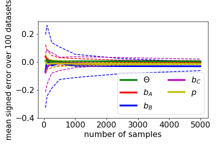
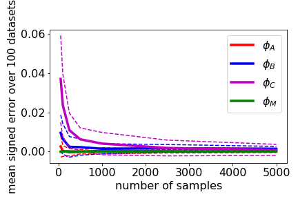
Figure 3: For each parameter, the mean signed error over the simulated datasets decreases with the size of the simulated datasets. Dotted lines denote 1 standard deviation.

Here, we examine the ability of our model to recover the model parameters as the amount of data simulated using those parameters grew. We chose a single set of shared model parameters and hyperparameters $\mu_{A},\mu_{B},\mu_{C}$. Then, we performed the following for several values of $N$, the number of patients in a simulated dataset: We simulated 100 datasets, where for each dataset we used that set of chosen parameters to simulate observed function values $y_{i}(t)$ for $N$ patients at times $t\in\{1,2,4,8,12,18,24,30,36,42,48\}$, the same times at which data were observed in the prostate cancer dataset. For each dataset, we obtained for each parameter a point prediction as its posterior median, and calculated two quantities: the signed error and unsigned error. Figure 3 shows the mean and standard deviation of the signed error across the 100 datasets for each parameter, for various values of N (N$\in\{50,100,250,500,1000,2500,5000\}$). Please see Figure 10 of the Supplementary Materials for the analogous information, for the unsigned error. Note that Figure 3 thus shows the bias and variance of the point estimates of the parameters, with the estimator being their respective posterior medians.

The set of parameters we used was simply one that was not pathological. We used $b_{A}=1,b_{B}=2,b_{C}=3,\theta=0.1,p=0.3,\phi_{A}=\phi_{B}=\phi_{C}=\phi_{M}=0.01$, and $\mu_{A}=0.4,\mu_{B}=0.7,\mu_{C}=5$. We assume only 1 feature, which for each sample is generated from a unit normal distribution. For inference, we set $s_{A}=s_{B}=s_{C}=1$, $\lambda_{A}=\lambda_{B}=\lambda_{C}=10$ and $\lambda_{M}=10$. To obtain posterior samples, we used Stan (Hoffman and Gelman, 2011), obtaining 2500 samples from each of 4 chains with no thinning, using 2500 burn-in steps. We assessed convergence both by using the Gelman statistic (Gelman and Rubin, 1992) and visual examination of the traces for each parameter. We checked that in fitting the model to each simulated dataset, the maximum Gelman statistic over parameters was less than $1.2$. The meaning of errors in the regression parameter is provided by Equations 4.2-4.4, and the meaning of errors in the spread parameters $\phi_{A},\phi_{B},\phi_{C},\phi_{M}$ is provided by the plots of beta and gamma distributions in Figures 6 and 8 of the Supplementary Materials.

6 Analysis of Prostate Cancer Dataset

6.1 Dataset Description

Our data comes from a study (Gore and others, 2009, 2010) that prospectively tracked the sexual function as measured using the UCLA Prostate Cancer Index (Litwin and others, 1998) of 304 patients who underwent radical prostatectomy to treat clinically localized prostate cancer. After applying dataset filters as detailed in Section 3 of the Supplementary Materials, data from 237 patients is retained. Their sexual function levels were collected right before treatment and over a 48-month post-treatment study period via mailed surveys at 1,2,4,8,12,18,24,30,36,42, and 48 months after their respective treatments, and missing data was due to lack of survey response. The Prostate Cancer Index, derived from answers to a series of multiple choice questions, is a numerical measure of a patient’s level of sexual function that lies between 0 and 100, which we scale to the unit interval. Various patient covariates were collected at time of treatment, including age, cancer grade/stage, physical/mental condition, uninary/bowel function, and comorbidity count.

Prostate cancer patients’ post-prostatectomy sexual function outcomes can be modulated by non-mandatory post-prostectomy treatments such as the use of an erectile aid. As such additional treatments are non-standard, our goal in this particular analysis is to model the sexual function outcomes for patients who would not receive them. Furthermore, we are not interested in modeling the post-prostatectomy sexual function of patients whose sexual function prior to the potential prostatectomy is already close to 0, as such patients’ post-treatment sexual function would be expected to remain constant afterwards, following a different model that is uninteresting to analyze. Thus, we define the target population of this model to be patients considering a prostatectomy, who satisfy the following two properties: firstly, they would not use any additional remedial treatments post-prostatectomy, such as an erectile aid, and secondly, they would have a non-neglible level of sexual function prior to receiving the potential prostatectomy. The dataset filters we applied retain members of this target population.

6.2 Choosing Features

To identify potential correlates of recovery curve shapes, for every patient, we used curve fitting to find the $A,B,C$ parameters corresponding to their post-event recovery shapes. We made scatter plots of each of those parameters against all available covariates to identify ones that correlated with curve parameters, and identified the pre-treatment sexual function level (referred to as “init” in all figures) and patient age (at treatment time) to be the 2 covariates most strongly correlated with curve parameters. From the scatter plots (in Figure 11 of the Supplementary Materials), we saw the relationship between those 2 covariates and curve parameters is likely nonlinear. Thus we created binned categorical features based on age and pre-treatment function level. The bins for the categorical features we used were as follows:

• age (in years): 0 to 55, 55 to 65, 65+

• pre-treatment function level: 0 to 41, 41 to 60, 60 to 80, 80 to 100

We note that such subdivisions matches with the urologist co-author’s clinical experience regarding how urologists categorize age and pre-treatment function level.

Thus, in our model, patients belong to 1 of 12 classes, depending on into which of the three age groups they fall into, and which of the four intervals their pre-treatment sexual function level lies. These features were normalized. To visualize the effect of these 2 covariates on recovery shape from another view, we stratified the patients by age category and pre-treatment sexual function level category, and plotted (see Figure 12 of the Supplementary Materials) the average shape of the patients in each category.

6.3 Fitting Our Model

Now, we describe how we chose hyperparameters, and the fitting of the model. To choose $\mu_{A},\mu_{B},\mu_{C}$, which describe the average recovery shape for the “average” patient in the target population, we fit a recovery shape using our parametric form to the training fold-wide average scaled function value shown in Figure 1(a) (labeled “average shape”). The values we used for the remaining hyperparameters were $s_{A}=s_{B}=s_{C}=1$ and $l_{A}=l_{B}=l_{C}=l_{M}=10$. We show in Section 6.1 of the Supplementary Materials that out-of-sample performance (as described in Section 6.4) is not sensitive to the particular choice of those hyperparameters.

To fit the model, we used Stan (Hoffman and Gelman, 2011), for each of 4 chains, running 2500 steps with 2500 burn-in steps and no thinning, and assessed convergence using the Gelman statistic (Gelman and Rubin, 1992) (The maximum value of the Gelman statistic over all parameters was 1.11). Please see Section 6.3 of the Supplementary Materials for posterior predictive checks.

6.4 Out-of-Sample Performance

We measure the performance of our model by its ability to predict $y_{i}(t)$, the observed function values. We obtain a point prediction of $y_{i}(t)$, denoted $\hat{y}_{i}(t)$, via the median of the posterior distribution of $f_{i}(t)$, the “underlying” function value. The loss function we use to measure performance was absolute prediction error: the absolute difference between $y_{i}(t)$ and $\hat{y}_{i}(t)$. To measure out-of-sample performance, we performed 5-fold cross-validation, obtaining, for each test sample, point predictions from our model, and examined the average, over the test folds, of loss at a given time as measured by absolute prediction error. (The average loss at time $t$ for a test fold consisting of the patient index set $I$ for which function values were recorded at time $t$ is $\tfrac{1}{|I|}\sum_{i\in I}|\hat{y}_{i}(t)-y_{i}(t)|$ where $\hat{y}_{i}(t)$ is the point prediction of the function level of patient $i$ at time $t$ and $|I|$ is the size of index set $I$.) In particular, the entire time series for patients in the testing folds are predicted given the entire time series of the patients in the training fold. Data from the early part of one patient’s time series is not used to predict the same patient’ s future values. We plot, over time, the out-of-sample performance of our model, as well as that of two baseline models in Figure 4(a). Note that all comparison models, like our model, first predict the patient’s scaled function values, and then multiply it by their pre-treatment value to obtain a prediction of absolute function value. To compare the improvement of our method to the status quo, in which a doctor merely tells a patient the population-wide average shape, we plotted the performance of simply predicting a patient to have the average recovery shape, labelled “mean”. We compared the performance of our model to a timewise scaled regression that, at each of the 11 common timepoints, uses a separate generalized linear regression model to relate the scaled function value at the timepoint to patient features. This model, labelled “scaled regression”, uses a logistic inverse link function and assumes a normal response distribution. Finally, because of the high variance in our data, we show for comparison the in-sample performance of a model that is prone to overfitting. This model, labelled “median”, in order to make a prediction for a patient at a given time, looks at which of the 12 patient classes the patient belongs to and then calculates the median scaled function value, at the given time, of patients who belong to that patient class, over the entire dataset. As can be seen in Figure 4(a), the out-of-sample performance of our model is roughly equivalent to that of the scaled regression model, though our model is more interpretable. Error bars show the variance in estimates of the expected loss at each time.

6.5 Interpretability of Model

Our model achieves out-of-sample performance comparable to that of the timewise scaled regression described in Section 6.4. However, our model produces much more easily understood predictions, outputting a distribution over time series consisting solely of recovery curves, so that they are smoothly increasing monotonically towards an asymptote, and do not exceed the pre-treatment value. In contrast, the timewise scaled regression model produces a time series that is not guaranteed to be smooth or monotonically increasing. In addition to matching prior expectations, our model’s predictions are more quickly processed by the patient, which, as our references to interpretability indicated, are crucial in a clinical setting. To illustrate, in Figure 4(b) for several of the 12 classes of patients, we plot the scaled function values produced by scaled timewise regression, the distribution over $f_{t}$ from our model, and the timewise median of that distribution. A patient, expecting to see a recovery curve, can with a quick glance of the red curves (timewise median of our predictions), pick up what the initial drop, asymptotic drop, and recovery rate of their predicted recovery curve are. On the other hand, with the scaled timewise regression, the patient tries to extrapolate what those same quantities are from the jagged predictions, finds it hard to do so, wondering whether the fluctuations are a real trend or just noise.

Furthermore, we have designed our model so that prediction uncertainty is easily interpretable when a patient’s posterior distribution of curves is plotted. Because we encourage the a patient’s recovery curve parameter distribution to be unimodal in the posterior, we expect the pointwise distribution of curve values, namely that of $f_{t}$, to be unimodal. This is why in Figure 4(b), the distribution of curves appears clustered about the red curve. It is important that one can visually extract from a plot of posterior distribution of curves a single most likely curve. Then, such a plot can be interpreted as giving a single curve prediction, along with the uncertainty in that prediction. On the other hand, if the posterior distribution of curves were clustered around, say, two curves, there would be no such clear interpretation.

6.6 Dependence of Recovery Shape on Covariates and Comparison with Literature

Our analysis teases apart the dependence of recovery shape on age and pre-treatment value. In Figure 5(a), we examine the effect of patient age on recovery curve shape by stratifying those curves by pre-treatment level. We find when pre-treatment level is controlled for, patients younger than 55 years of age have a smaller asymptotic drop in sexual function level, proportional to their pre-treatment level. (We performed a one-sided z-test that the scaled function value at 48 months for patients younger than 55 years of age was larger than those not; p-value = $.005$.) This effect is diminished for patients with pre-treatment level higher than 0.80. When pre-treatment level is not controlled for, the asymptotic proportional drop in function level for younger patients is lower. In both cases, the proportional initial drop in function level does not depend on age. In Figure 5(b) we examine the effect of pre-treatment sexual function level on recovery shape by stratifying those curves by age. We find that when age is controlled for, patients with pre-treatment level higher than 0.80 have a smaller asymptotic drop in function level, proportional to their pre-treatment level. (One sided z-test p-value = $4.17\text{\times}{10}^{-7}$.) However, this effect is diminished for patients younger than 55. The proportional initial drop in function depends mildly on pre-treatment level.

Unlike past methods, which have mostly focused on modeling a continuous or binary measure of sexual function at a single fixed time, our model makes predictions of the entire post-treatment function trajectory. Regardless, we can still compare our findings to them. Past work that modeled a continuous measure of sexual function found that lower age and higher pre-treatment sexual function level are statistically linked to higher absolute levels of that measure (Talcott and others, 2003), and that lower age is linked to a smaller change in that measure of function level (Sanda and others, 2008). Likewise, when a binary indicator of satisfactory sexual function has been logistically regressed against patient covariates, lower age (Regan and others, 2011; Ayyathurai and others, 2008) and higher pre-treatment function level (Regan and others) have been found to lead to a higher probability of having satisfactory sexual function. One can conclude from these past statistical analyses, as well as model-free data analyses (Rabbani and others, 2000; Michl and others, 2006), that lower age and higher pre-treatment sexual function level, by any measure, are linked to higher post-treatment sexual function level, agreeing with our findings. Though, we stress that unlike any previous analysis, we model the link between patient features and longitudinal sexual function levels proportional to the pre-treatment level.

7 Conclusion

We presented a Bayesian model that can be used to predict recovery curves, which arise in many medical contexts. Our overarching goal is to facilitate the flow of information from the data to the user, who may not be statistically inclined. Towards this end, we impart interpretability to both the model and its output, a model that is easily explained and produces believable outputs is more clinically applicable. In particular, our model predicts quantities that are of natural interest, and guarantees that its output is in fact the recovery curve that we assume a domain expert to expect of a prediction. Furthermore, our model is designed for easy visualization of predictions and the associated uncertainty, as we encourage the posterior distribution over recovery curves to have a clear ’mode’. We used our model to analyze the impact of prostatectomy on a patient’s post-treatment sexual function trajectory, and characterized the extent of that impact on patient age and pre-treatment sexual function level, producing conclusions that agree with and supplement past findings. We believe our model can provide insights in other medical domains as well.

8 Supplementary Materials

The Supplementary Materials are available at http://biostatistics.oxfordjournals.org. It contains details of the reparameterizations of the beta and gamma distributions, exploratory plots and details of filtering of the prostatectomy dataset, as well as an additional simulation study. Furthermore, it contains further analysis of the prostatectomy dataset as it relates to our model: posterior predictive checks and sensitivity of results to hyperparameters and measurement error in the pre-treatment function level. Finally, it contains high resolution plots of the posterior predictive distribution for the patients in the prostatectomy dataset. Simulated data and code are available at https://github.com/fultonwang/recovery_curve.

9 Acknowledgements

This work was supported by National Science Foundation CAREER grant IIS-1053407 to C. Rudin and National Science Foundation grant DMS-1737673 to T. McCormick. We thank Dr. Jim Michaelson of Massachusetts General Hospital for helpful discussions.

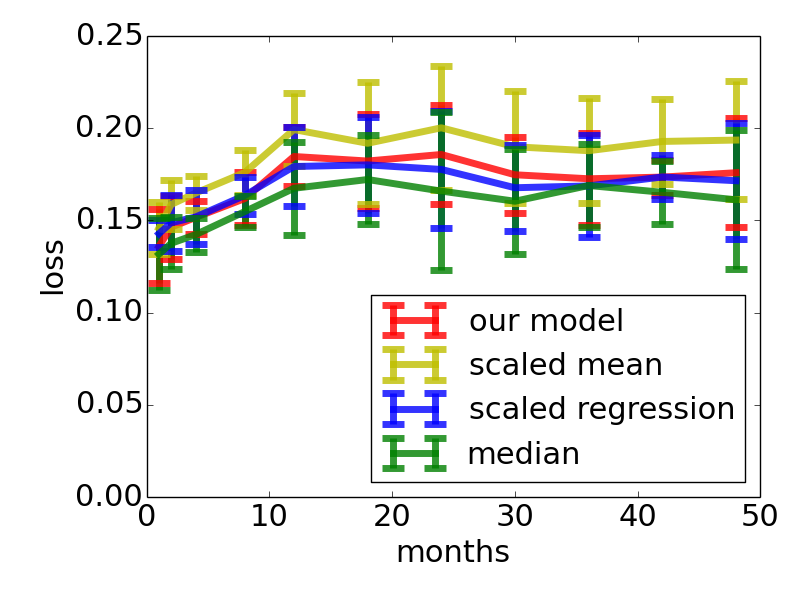
(a) The out-of-sample performance of our model is comparable to that of timewise scaled regression, and approaches the in-sample performance of “median”, a method prone to overfitting.

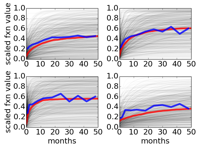
(b) The posterior predictive distribution over recovery curves (black) and timewise medians of it (red) convey more plausible predictions than that of timewise scaled regression (blue), whose prediction is not guaranteed to be a recovery curve.

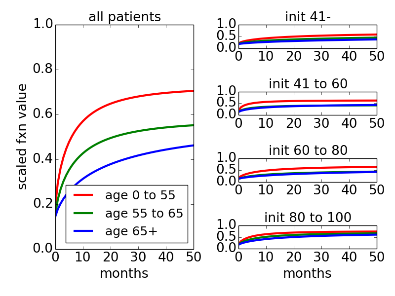
(a) age trend

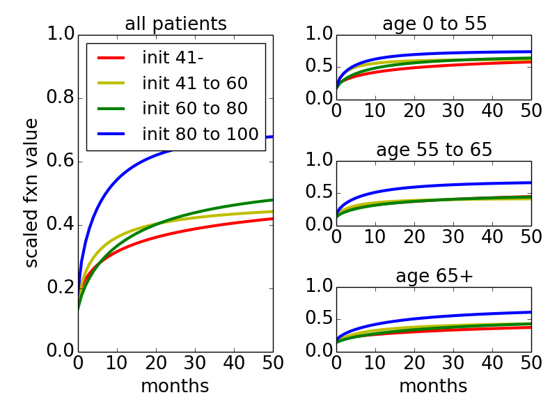
(b) pre-treatment level trend

Figure 5: Our model identifies the relationship between pre-treatment level, age, and a patient’s latent recovery shape.

Supplementary Material

1 Reparameterization of beta and gamma distributions

Our $\operatorname{beta}_{m,\phi}(\cdot,\cdot)$ parameterization is based on the traditional $\operatorname{beta}_{\alpha,\beta}(\cdot,\cdot)$ parameterization. A $\operatorname{beta}_{\alpha,\beta}(\alpha^{\prime},\beta^{\prime})$ distribution is unimodal with mode $\frac{\alpha^{\prime}-1}{\alpha^{\prime}+\beta^{\prime}-1}$ if and only if $\alpha^{\prime}>1,\beta^{\prime}>1$. Making the substitution $\alpha=1+sm$ and $\beta=1+s(1-m)$, we obtain the parameterization $\operatorname{beta}_{m,s}(m^{\prime},s^{\prime})=\operatorname{beta}_{\alpha,\beta}(1+s^{\prime}m^{\prime},1+s^{\prime}(1-m^{\prime}))$. It can be easily checked that a $\operatorname{beta}_{m,s}(m^{\prime},s^{\prime})$ distribution, for all $m^{\prime}$, is unimodal with mode $m^{\prime}$ if and only if $s^{\prime}>0$. Finally, we make the substitution $s=\frac{1}{\phi}-1$ to obtain the desired $\operatorname{beta}_{m,\phi}(\cdot,\cdot)$ parameterization, where a $\operatorname{beta}_{m,\phi}(m^{\prime},\phi^{\prime})$ distribution, for all $m^{\prime}$, is unimodal with mode $m^{\prime}$ if and only if spread parameter $\phi^{\prime}\in(0,1)$:

$$\operatorname{beta}_{m,\phi}(m^{\prime},\phi^{\prime})=\operatorname{beta}_{\alpha,\beta}\left(1+\left(\frac{1}{\phi^{\prime}}-1\right)m^{\prime},1+\left(\frac{1}{\phi^{\prime}}-1\right)\left(1-m^{\prime}\right)\right).$$ (1.1)

Examples of such beta distributions are in Figure 6, and the regions of unimodality for our beta distribution parameterization compared to the traditional one are in Figure 7.

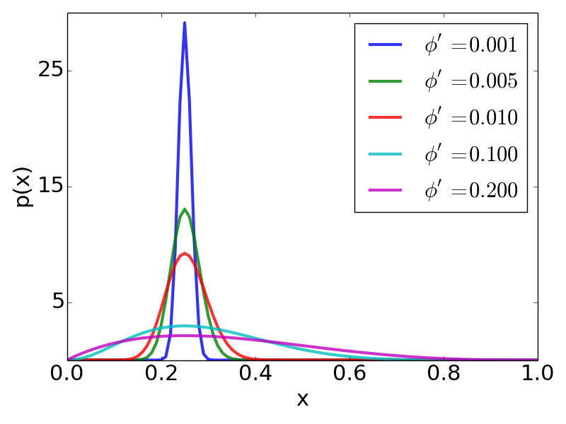
(a) pdfs of $\operatorname{beta}_{m,\phi}(m^{\prime},\phi^{\prime})$ distributions with $m^{\prime}=0.25$

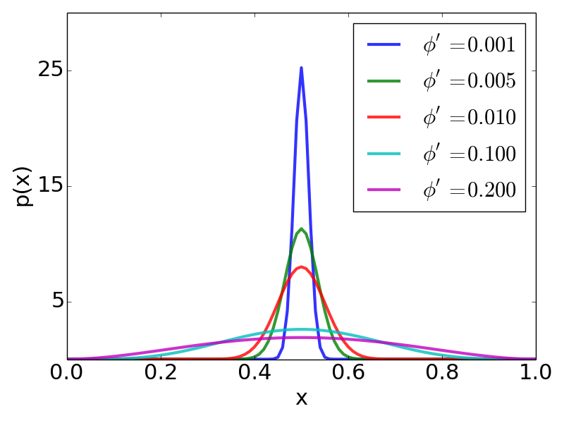
(b) pdfs of $\operatorname{beta}_{m,\phi}(m^{\prime},\phi^{\prime})$ distributions with $m^{\prime}=0.5$

Figure 6: Illustrations of our parameterization of the beta distribution

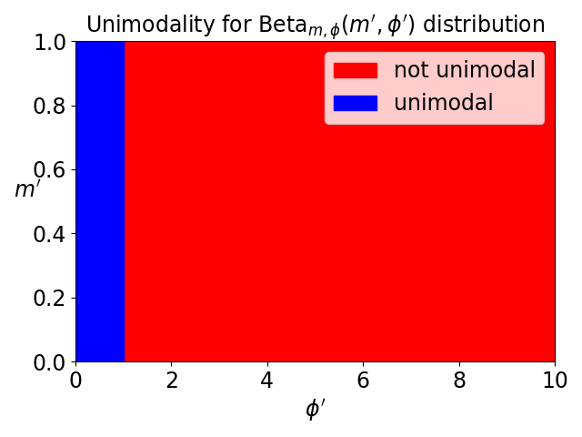
(a) A $\operatorname{beta}_{m,\phi}(\cdot,\cdot)$ parameterization suits our purposes because for a given $\phi^{\prime}<1$ (a constraint we enforce), a $\operatorname{beta}_{\mu,\phi}(m^{\prime},\phi^{\prime})$ distribution is unimodal for all $m^{\prime}$.

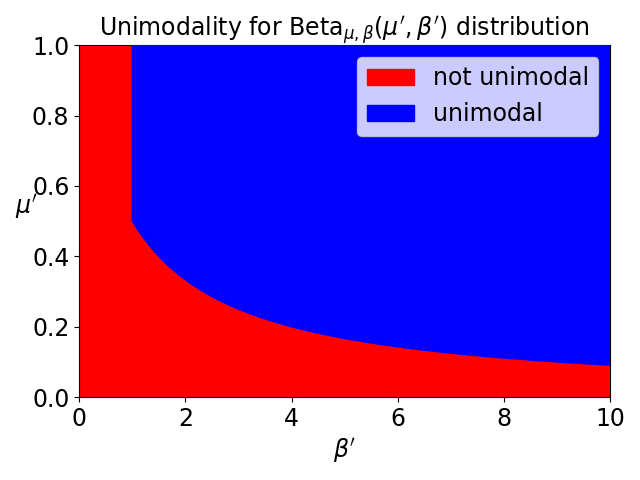
(b) A $\operatorname{beta}_{\mu,\beta}(\cdot,\cdot)$ parameterization is unsuitable because for a given $\beta^{\prime}$, there exists $m^{\prime}$ such that a $\operatorname{beta}_{\mu,\beta}(m^{\prime},\beta^{\prime})$ distribution is not unimodal.

Figure 7: Regions of unimodality for two different beta distribution parameterizations

Our $\operatorname{gamma}_{m,\phi}(\cdot,\cdot)$ parameterization is based on the traditional $\operatorname{gamma}_{\alpha,\beta}(\cdot,\cdot)$ parameterization. A $\operatorname{gamma}_{\alpha,\beta}(\alpha^{\prime},\beta^{\prime})$ distribution is unimodal with mode $\frac{\alpha^{\prime}-1}{\beta^{\prime}}$ if and only if $\alpha^{\prime}>1$. Substituting $\beta=\frac{\alpha-1}{m}$ and $\alpha=\frac{1}{\phi}$, we obtain the $\operatorname{gamma}_{m,\phi}(\cdot,\cdot)$ parameterization. A $\operatorname{gamma}_{m,\phi}(m^{\prime},\phi^{\prime})$ distribution is unimodal with mode $m^{\prime}$ if and only if spread parameter $\phi^{\prime}\in(0,1)$:

$$\operatorname{gamma}_{m,\phi}(m^{\prime},\phi^{\prime})=\operatorname{gamma}_{\alpha,\beta}\left(\frac{1}{\phi^{\prime}},\frac{\nicefrac{{1}}{{\phi^{\prime}}}-1}{m^{\prime}}\right).$$ (1.2)

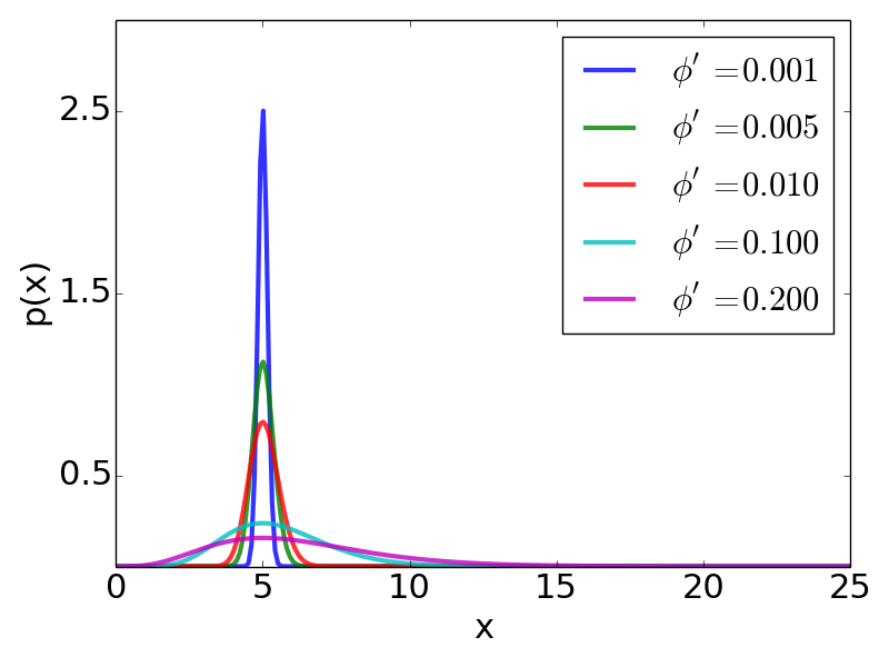
(a) pdfs of $\operatorname{gamma}_{m,\phi}(m^{\prime},\phi^{\prime})$ distributions with $m^{\prime}=15$

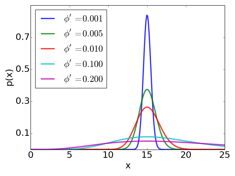
(b) pdfs of $\operatorname{gamma}_{m,\phi}(m^{\prime},\phi^{\prime})$ distributions with $m^{\prime}=15$

Figure 8: Illustrations of our parameterization of the gamma distribution

Examples of such gamma distributions are in Figure 8.

Note that both a $\operatorname{beta}_{m,\phi}(m^{\prime},\phi^{\prime})$ and $\operatorname{gamma}_{m,\phi}(m^{\prime},\phi^{\prime})$ have variance increasing in $\phi^{\prime}$. That is why we regard $\phi^{\prime}$ as a spread parameter.

2 Additional Simulation Studies

Here, we examine our model’s robustness to simulated data violating the underlying model assumptions. We performed the following for various values of $M$, the number of noise samples: We simulated a single dataset by first simulating observed function values for $5000$ samples using the same parameters as in the first experiment. However, then we added to the dataset an additional $M$ noise samples whose observed function values which were not generated from the model. Instead, for those $M$ noise samples, at each time point for which the function value is observed, we drew the observed value uniformly from the unit interval. For inference, we used the same hyperparameters, sampling method, and convergence diagnostics as before. We then calculated, for each parameter, the error: the signed difference between its median posterior distribution and the true value used to simulate (part of) the dataset. In Figure 9, we plot for each parameter this signed difference (as well as the 25-th and 75-th percentile of the error) as $M$, the number of noise data samples, varies. As expected, the magnitude of this error is increasing in $M$.

We also include here an additional plot describing the results of the simulation study in Section 5 of the manuscript. Recall that the purpose of the simulation study was to examine the ability of our model to recover the model parameters as the amount of data simulated using those parameters grew. We chose a single set of shared model parameters and hyperparameters $\mu_{A},\mu_{B},\mu_{C}$. Then, we performed the following for several values of $N$, the number of patients in a simulated dataset: We simulated 100 datasets, where for each dataset we used that set of chosen parameters to simulate observed function values $y_{i}(t)$ for $N$ patients at times $t\in\{1,2,4,8,12,18,24,30,36,42,48\}$, the same times at which data were observed in the prostate cancer dataset. For each dataset, we obtained for each parameter a point prediction as its posterior median, and calculated the unsigned error. Figure 10 shows the mean and standard deviation of the signed error across the 100 datasets for each parameter, for various values of N (N$\in\{50,100,250,500,1000,2500,5000\}$). Note that in the manuscript, we had shown the analogous results for the signed error. Please see the manuscript for further details on the values of the parameters used to simulate the data as well as the inference method.

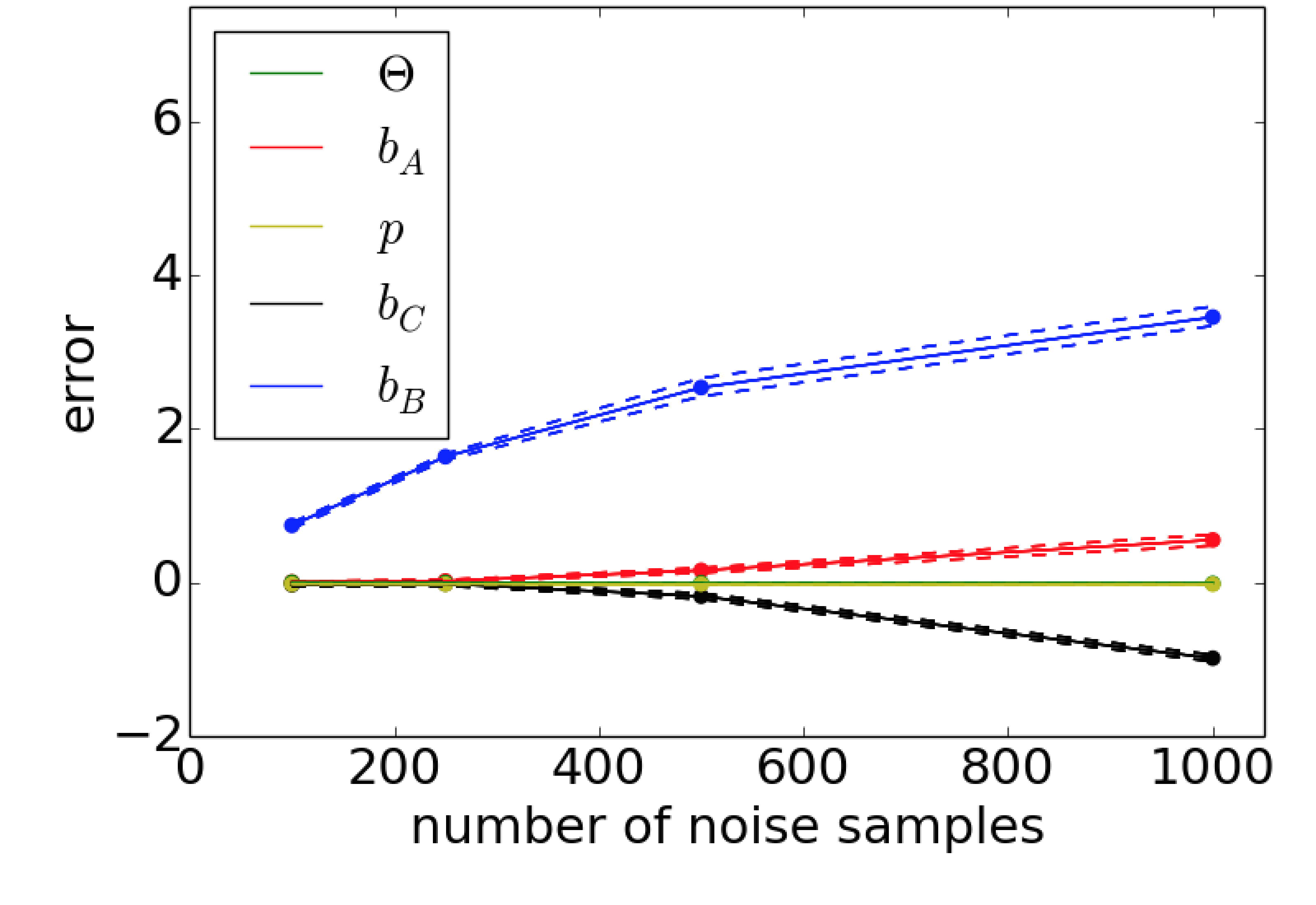
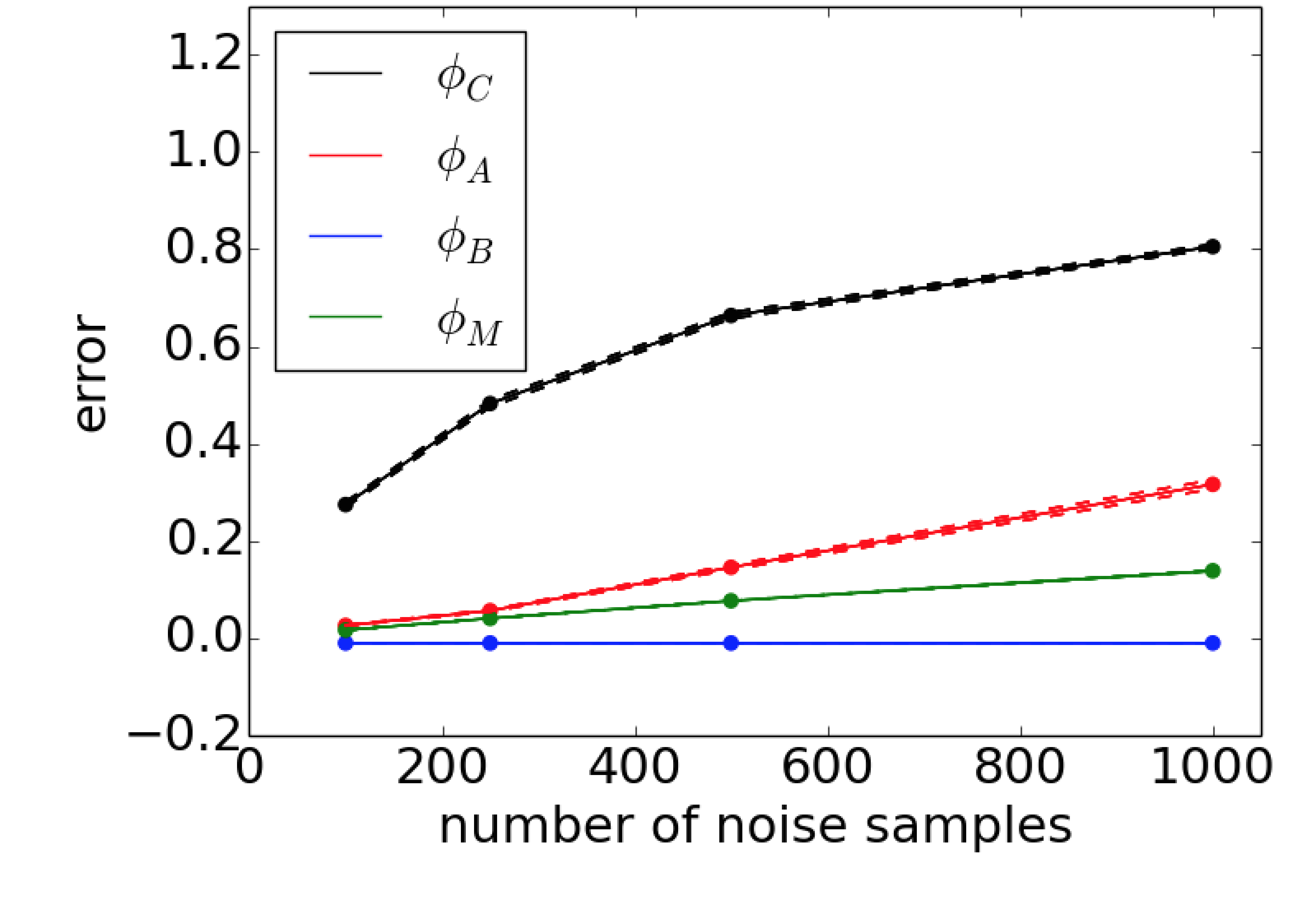
Figure 9: For each parameter, the magnitude of the difference between posterior median parameter and true value increases with amount of noise data.

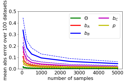
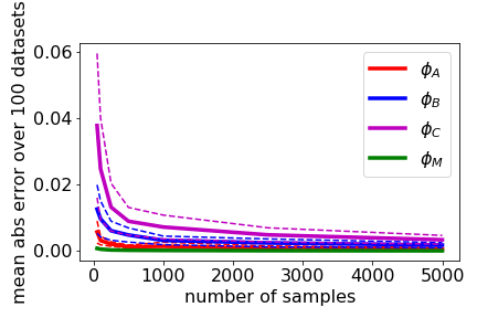
Figure 10: For each parameter, the mean absolute error over the simulated datasets decreases with the size of the simulated datasets. Dotted lines denote 1 standard deviation.

3 Dataset Filtering

We apply two filters to our dataset such that the retained patients possess the properties required of the target population, retaining 237 out of the original 304 patients’ data. We note that while our target population includes patients merely considering a prostatectomy, our actual dataset only contains data from patients who actually underwent a prostatectomy. Our assumption is that patients passing the two filters will belong to the target population, not differing from it on any unmeasured covariates impacting sexual function trajectory. For the first filter, we removed 17 patients whose pre-treatment sexual function level was less than 0.1, as our target population was defined to have a non-negligible pre-treatment function level. Secondly, as our dataset contains patients who both did and did not use an erectile aid post-treatment, we wish to remove patients who did use an erectile aid. Unfortunately, our dataset did not record whether an aid was used, and we had to instead infer its usage from the data, based on a criteria set by the urologist co-author: For the second filter, we removed patients whose representative curve, obtained by fitting a curve (under least squares error, where the asymptotic level was not constrained) to their data points, was, at 48 months post-treatment (the last time for which data was available), higher than their pre-treatment value. Doing so removed an additional 50 patients, so that our final retained dataset contained 237 out of the original 304 patients. This second filter is justified by the urologist co-author’s past clinical experience that a prostatectomy patient who does not use an erectile aid has a negligible chance of having their long-term sexual function exceed that pre-treatment. Thus, this filter will remove a neglible number of patients that did not use an erectile aid, though actually it retains some patients not in the target population - those who used an aid, but whose sexual function did not improve long-term.

4 Exploratory Plots

To identify potential correlates of recovery curve shapes, for every patient, we used curve fitting to find the $A,B,C$ parameters corresponding to their post-event recovery shapes. We made scatter plots of each of those parameters against all available covariates to identify ones that correlated with curve parameters, and identified the pre-treatment sexual function level (referred to as “init” in all figures) and patient age (at treatment time) to be the 2 covariates most strongly correlated with curve parameters. The scatter plots relating curve parameters and those 2 covariates are in Figure 11, and guided the creation of binned categorical features based on patient age and pre-treatment function level. To visualize the effect of these 2 covariates on recovery shape from another view, we stratified the patients by age bin and pre-treatment sexual function level bin, and plotted in Figure 12 the average shape of the patients in each bin. (The ranges of the of the bins we used in the categorical features are contained in the figure.)

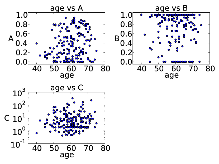
(a) parameters vs age

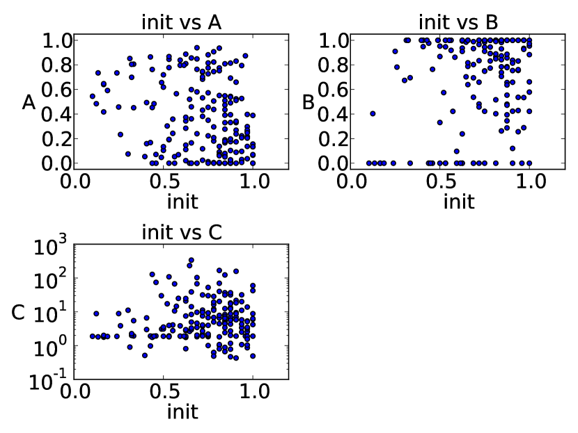
(b) parameters vs pre-treatment level

Figure 11: The three curve parameters show some dependence on a patient’s age and pre-treatment sexual function value.

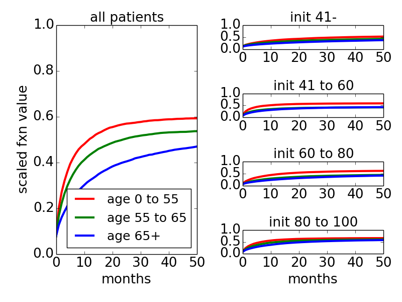
(a) Averaged scaled function values stratified by age

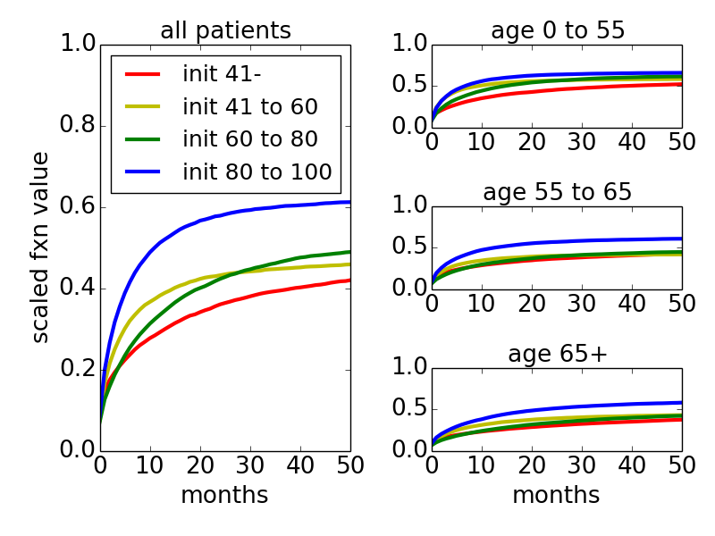
(b) Averaged scaled function values stratified by pre-treatment value

Figure 12: Plotting the average scaled function values over the dataset stratified by age and pre-treatment sexual function value suggests the dependence of latent recovery shapes on age and pre-treatment value.

5 Modeling Scaled Function Values

In general there are 2 potential approaches to modeling patients’ absolute function values - we can do so directly, or instead model their scaled function value (absolute function value divided by pre-treatment function value), and then scale it by their pre-treatment value. As we take the latter approach, we examine the prostatectomy dataset to justify doing so, showing that naive models that model scaled function value have superior in-sample performance on the prostatectomy dataset to their unscaled analogue. The measure of performance we consider here and throughout the rest of the paper is loss as given by average absolute prediction error.

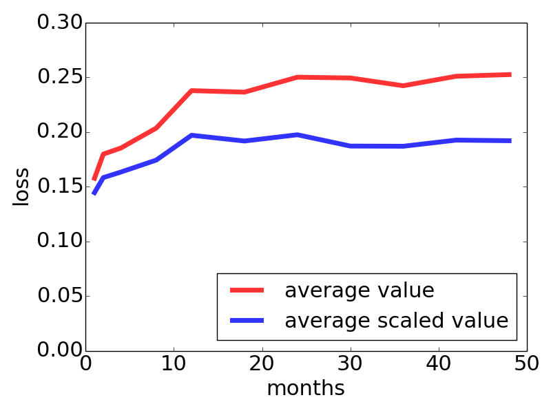
(a) covariate-independent models

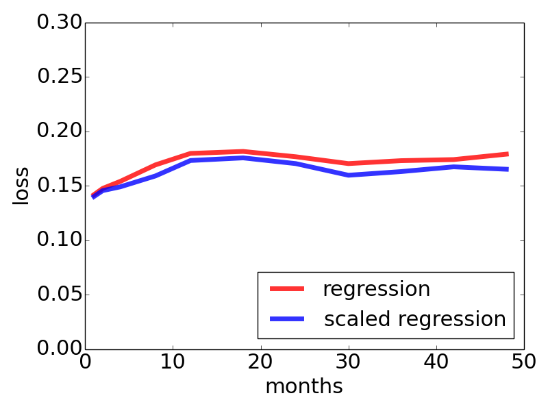
(b) regression models

Figure 13: In-sample performance is better when using models that model scaled function value as opposed to absolute function value.

First, we consider a baseline model where at each timepoint, each patient is predicted to possess the average absolute function value (over the dataset) at that timepoint (labeled “average value”). We compare its in-sample predictive performance (fit) to a model where each patient is predicted to have the average scaled function value at that timepoint (labeled “average scaled value”) in Figure 13(a). Next, we plot in Figure 13(b) the in-sample predictive performance of two analogous models that use separate generalized linear regression models at each of the 11 common timepoints to model a patient’s absolute and scaled function value, respectively, as a function of patient features. In other words, one model (labeled “regression”) regresses the absolute function value at each timepoint against patient features, and the other model (labeled “scaled regression”) regresses the scaled function value against features, and to obtain a prediction of absolute function value, assumes that a patient’s absolute function value is their scaled function value divided by their pre-treatment function value. The generalized linear regression models employ a logistic inverse link function and assume a normal response distribution. As can be seen, in both the cases, the models that predict scaled function value have superior predictive performance.

6 Additional Analysis of Prostatectomy Dataset

In the following subsections, we perform additional analysis of the prostatectomy dataset as it relates to our model.

6.1 Sensitivity of Out-Of-Sample Performance to Hyperparameters

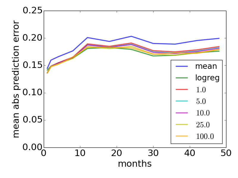
(a) Out-of-sample performance as the tied values of $l_{A},l_{B},l_{C}$ vary. The numerical labels indicate the tied value of $l_{A},l_{B},l_{C}$.

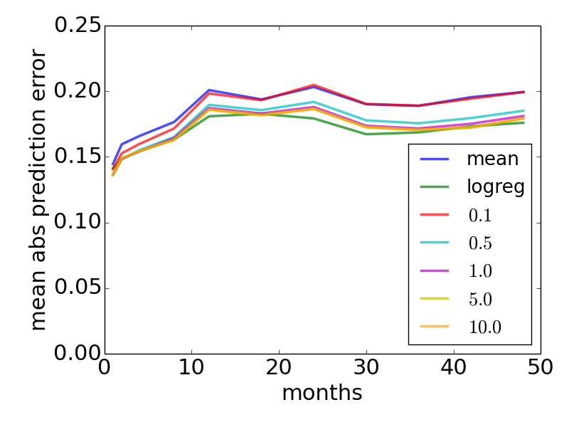
(b) Out-of-sample performance as the tied values of $s_{A},s_{B},s_{C}$ vary. The numerical labels indicate the tied value of $s_{A},s_{B},s_{C}$.

Figure 14: Sensitivity of out-of-sample performance to hyperparameters.

We provide a sense in Figures 14(a) and 14(b) how out-of-sample performance changes with the values of hyperparameters $s_{A},s_{B},s_{C}$ and $l_{A},l_{B},l_{C}$. The joint setting of those hyperparameter values we used in the analysis of the prostatectomy data was $l_{A}=l_{B}=l_{C}=10$, $s_{A}=s_{B}=s_{C}=1.0$ (and $l_{M}=10$, though performance was not sensitive to $l_{m}$). In Figure 14(a), we tie $\l_{A}=\l_{B}=l_{C}$, and illustrate how out-of-sample performance changes as the tied value of $l_{A},l_{B},l_{C}$ changes, with the remaining hyperparameters set to their original values. In Figure 14(b), we tie $s_{A}=s_{B}=s_{C}$ and illustrate how out-of-sample performance changes as the tied value of $s_{A},s_{B},s_{C}$ changes, with the remaining hyperparameters set to their original values. In both figures, we also include for comparison the performance of the “scaled mean” (denoted by “mean” in the figure) and “scaled regression” (denoted by “logreg” in the figure) models as described in Section 6.4 of the main text.

6.2 Sensitivity of posterior predictive variance to hyperparameters

Here, we examine the sensitivity of posterior predictive variance to variance hyperparameters $l_{A},l_{B},l_{C}$. In particular, we fix $s_{A}=s_{B}=s_{C}=1.0$ and $l_{m}=10$. Then, for several values of $v$, we set $l_{A}=l_{B}=l_{C}=v$, and for each time point $t$ for which there was recorded data, calculated the following: for each patient $i$ in the dataset, we calculated the standard deviation of the posterior predictive distribution of their “underlying” function value at time $t$, $f_{i}(t)$ , and then averaged these standard deviations over the entire dataset to get the mean standard deviation of the posterior predictive distribution at time $t$. In Figure 15, we plot, for several values of $v$ (the legend indicates $v$), the mean posterior standard deviation over time.

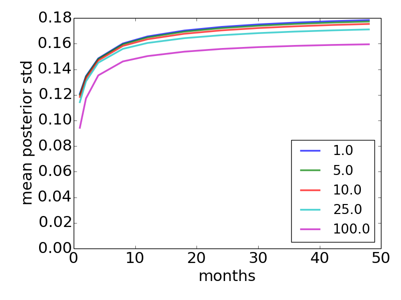
Figure 15: The standard deviation of the posterior predictive distribution, averaged over the dataset, is robust to the tied value of $l_{A},l_{B},l_{C}$, indicated by the labels.

6.3 Posterior Predictive Checks

To assess model fit, we performed standard posterior predictive checks with the following test statistics of the data:

• average total drop: pre-treatment level minus level at the last available time, averaged over patients.

• average relative total drop: pre-treatment level minus level at the last available time, divided by pre-treatment level, averaged over patients.

• average initial drop: pre-treatment level minus level at the first available time, averaged over patients.

• average relative initial drop: pre-treatment level minus level at the first available time, divided by pre-treatment level, averaged over patients.

• average recovery: level at last available time minus level at first available time post-treatment, averaged over patients

• average relative recovery: level at last available time minus level at first available time post-treatment, divided by pre-treatment level, averaged over patients

In Figure 16, the distribution of the test statistic over replicate datasets is shown in red for each test statistic, as is the actual test statistic for the data in blue. We see that under the 3 test statistics that are defined relative to the pre-treatment value, the data are fit quite well. Though, this is less the case for the other 3 test statistics that are not defined relative to the pre-treatment value. However, we believe the pattern of recovery relative to the pre-treatment value is a more important feature of the data than the absolute pattern of recovery - this is in part why we chose to model the relative function level rather than the absolute function level.

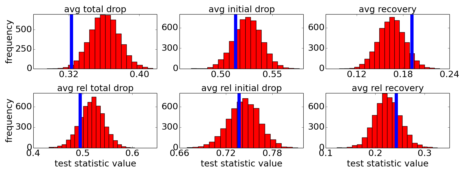
Figure 16: The empirical “relative” test statistics (blue vertical lines) are not extreme relative to that of the posterior over replicate datasets.

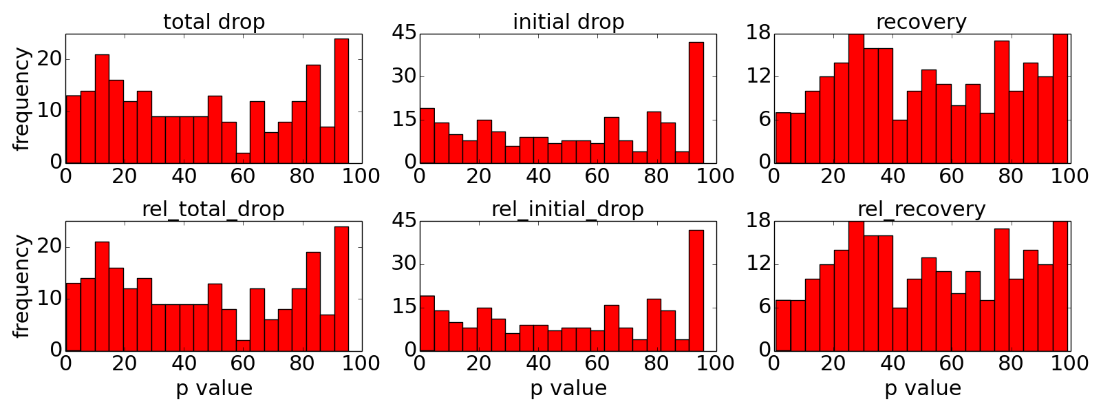
Figure 17: Most patients do not have an extreme empirical patient-specific test statistic relative to that of the posterior over replicate datasets, aside from the initial (relative) drop test statistic.

The above analysis addresses how the dataset as a whole is fit by the model. To assess how well individual patients’ data are fit by the model, we then defined a test statistic that is a function of only a single patient’s data. We then calculated the test statistic for each patient, thus obtaining 237 patient-specific test statistic values. Then, for each of the 237 patients, we calculated the p-value of their actual test statistic relative to that under replicate datasets simulated from the posterior. We then report in Figure 17 the distribution of the p-values, for that test statistic, over the patients in the dataset. These test statistics are the similar to before, except without averaging (they are all functions of a single patient’s data):

• total drop: pre-treatment level minus level at the last available time

• initial drop: pre-treatment level minus level at the first available time

• recovery: level at last available time minus level at first available time post-treatment

• relative total drop: pre-treatment level minus level at the last available time, divided by pre-treatment level.

• relative initial drop: pre-treatment level minus level at the first available time, divided by pre-treatment level.

• relative recovery: level at last available time minus level at first available time post-treatment, divided by pre-treatment level.

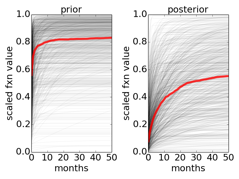
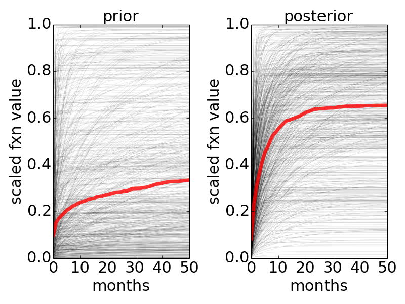
Figure 18: The prior vs posterior predictive distribution for 2 patients.

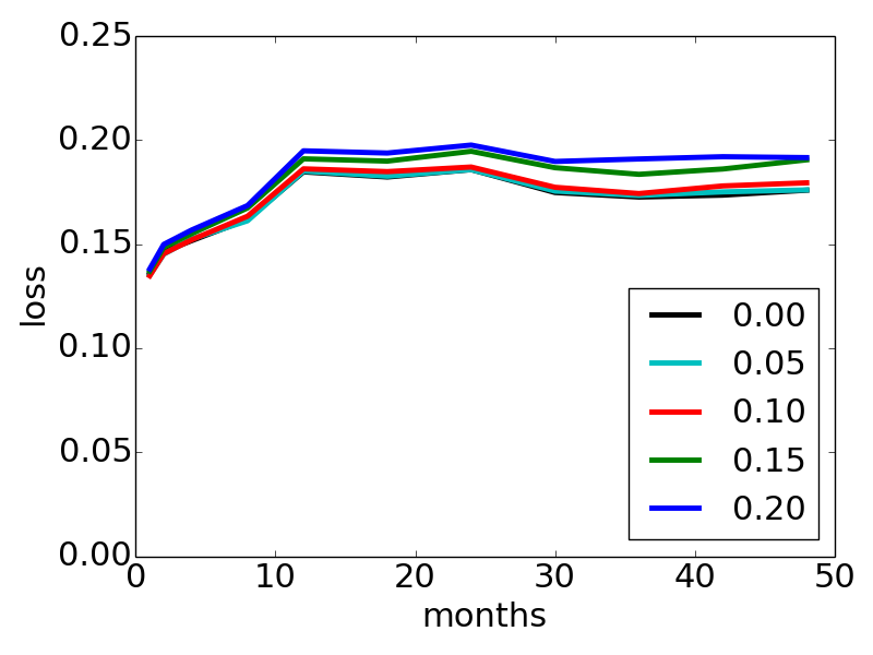
Figure 19: Predictive performance is robust to moderate measurement error in pre-treatment function level. Labels indicate the standard deviation of the perturbation noise distribution.

We see that for most patients, their (relative) total drop and (relative) recovery are not too extreme relative to the respective values in the replicate datasets. However, for for roughly 45 patients, their (relative) initial drop was at the 95th percentile of the respective initial drops in the replicate datasets, indicating that for those patients, their initial drop was greater than that predicted by the fit model. In fact, every single one of those 45 patients reported a sexual function value of exactly 0 at the first time for which data was available post-treatment. The likelihood allows the reported values, $y^{(i)}(t)$, to take on a value 0, with a probability that is constant across patients and time. One remedy would be to allow this probability to depend on patients and time, perhaps through the patient’s underlying function value, $f^{(i)}(t)$. However, as this feature of the data is likely noise, we opted not to do so.

6.4 Impact of the Data on Posterior

To understand the impact of the data on the posterior predictivedistribution, we illustrate for two patients their prior and posterior distribution over recovery curves in Figure 18.

6.5 Robustness to Measurement Error of Pre-treatment Function Level

In our model, we assume the pre-treatment function level is known. Here, we study the effect of measurement error in the pre-treatment function level on predictive performance. In particular, we performed an experiment where for each patient $i$ in our dataset, we obtained a draw from a normal distribution with mean 0 and fixed standard deviation (denoted $c$), and perturbed $S_{i}$ by that random amount (by choosing a perturbation direction of up or down randomly, then moving in that direction, reflecting off the boundaries of 0 and 1 if necessary) to obtain a single perturbed dataset. For a fixed value of $c$, we then obtained 8 perturbed datasets, and can then plot the cross validation performance over time (using the same evaluation metric as in evaluating out-of-sample performance in Section 6.4 of the main text), averaged over the 8 datasets. Figure 19 then shows the average cross validation performance, for several values of $c$.

6.6 Posterior Predictive Distributions for Patients

In the following pages, we display the posterior predictive distributions for all 12 types of patients in the prostatectomy dataset. Recall that patients belong to 1 of 3 strata based on their age, and 1 of 4 strata based on their pre-treatment level (see Figure 12 of the manuscript), which gives a total of 12 types of patients. The titles of the plots indicate the age and pre-treatment level strata of the patient whose posterior predictive distribution is displayed (the notation is the same as in Figure 13 of the manuscript.)

See pages - of all_12_predictions.pdf

References

- Ayyathurai and others (2008) Ayyathurai, R., Manoharan, M., Nieder, A. M., Kava, B. and Soloway, M. S. (2008). Factors affecting erectile function after radical retropubic prostatectomy: results from 1620 consecutive patients. BJU international 101(7), 833–6.
- Briganti and others (2011) Briganti, A., Gallina, A., Suardi, N., Capitanio, U., Tutolo, M., Bianchi, M., Salonia, A., Colombo, R., Di Girolamo, V., Martinez-Salamanca, J. I., Guazzoni, G., Rigatti, P. and others. (2011). What is the definition of a satisfactory erectile function after bilateral nerve sparing radical prostatectomy? The Journal of Sexual Medicine 8(4), 1210–7.
- Cai and Dunson (2007) Cai, B. and Dunson, D. B. (2007). Bayesian multivariate isotonic regression splines. Journal of the American Statistical Association 102(480), 1158–1171.
- Denison and others (1998) Denison, D. G. T., Mallick, B. K. and Smith, A. F. M. (1998). Automatic Bayesian curve fitting. Journal of Royal Statistical Society Series B.
- Descazeaud and others (2006) Descazeaud, A., Debré, B. and Flam, T. A. (2006). Age difference between patient and partner is a predictive factor of potency rate following radical prostatectomy. The Journal of Urology 176(6), 2594–2598.
- Eastham and others (2008) Eastham, J. A., Scardino, P. T. and Kattan, M. W. (2008). Predicting an optimal outcome after radical prostatectomy: the trifecta nomogram. The Journal of Urology 179(6), 2207–2211.
- Gelman and Rubin (1992) Gelman, A. and Rubin, D. (1992). Inference from iterative simulation using multiple sequences. Statistical Science 7(4), 457–511.
- Gore and others (2010) Gore, J. L., Gollapudi, K., Bergman, J., Kwan, L., Krupski, T. L. and Litwin, M. S. (2010). Correlates of bother following treatment for clinically localized prostate cancer. The Journal of Urology 184(4), 1309–15.
- Gore and others (2009) Gore, J. L., Kwan, L., Lee, S. P., Reiter, R. E. and Litwin, M. S. (2009). Survivorship beyond convalescence: 48-month quality-of-life outcomes after treatment for localized prostate cancer. Journal of the National Cancer Institute 101(12), 888–92.
- Hartzler and others (2015) Hartzler, A. L., Izard, J. P., Dalkin, B. L., Mikles, S. P. and Gore, J. L. (2015). Design and feasibility of integrating personalized pro dashboards into prostate cancer care. Journal of the American Medical Informatics Association.
- Hoffman and Gelman (2011) Hoffman, M. D. and Gelman, A. (2011). The No-U-Turn sampler: adaptively setting path lengths in Hamiltonian Monte Carlo. Journal of Machine Learning Research, 30.
- Jung and Wickrama (2008) Jung, T. and Wickrama, K. (2008). An introduction to latent class growth analysis and growth mixture modeling. Social and Personality Psychology Compass 2(1), 302–317.
- Litwin and others (1998) Litwin, M. S., Hays, R. D., Fink, A., Ganz, P. A., Leake, B. and Brook, R. H. (1998). The UCLA Prostate Cancer Index: development, reliability, and validity of a health-related quality of life measure. Medical Care 36(7), 1002–12.
- Mammen (1991) Mammen, E. (1991). Estimating a smooth monotone regression function. The Annals of Statistics 19(2), 724–740.
- Michl and others (2006) Michl, U. H. G., Friedrich, M. G., Graefen, M., Haese, A., Heinzer, H. and Huland, H. (2006). Prediction of postoperative sexual function after nerve sparing radical retropubic prostatectomy. The Journal of Urology 176(1), 227–31.
- Nayak and others (2015) Nayak, J. G., Hartzler, A. L., Macleod, L. C., Izard, J. P., Dalkin, B. M. and Gore, J. L. (2015). Relevance of graph literacy in the development of patient-centered communication tools. Patient Education and Counseling.
- Neelon and Dunson (2004) Neelon, B. and Dunson, D. B. (2004). Bayesian isotonic regression and trend analysis. Biometrics 60(2), 398–406.
- Potosky and others (2004) Potosky, A. L., Davis, W. W., Hoffman, R. M., Stanford, J. L., Stephenson, R., Penson, D. F. and Harlan, L. C. (2004). Five-year outcomes after prostatectomy or radiotherapy for prostate cancer: The Prostate Cancer Outcomes Study. Journal of the National Cancer Institute 96(18)(18), 1358–67.
- Rabbani and others (2000) Rabbani, F., Stapleton, A. M., Kattan, M. W., Wheeler, T. M. and Scardino, P. T. (2000). Factors predicting recovery of erections after radical prostatectomy. The Journal of Urology 164(6), 1929–34.
- Ramsay and Silverman (2002) Ramsay, J. O. and Silverman, B. W. (editors). (2002). Applied functional data analysis: methods and case studies, Springer Series in Statistics. New York, NY.
- Regan and others (2011) Regan, M. M., Cooperberg, M. R., Wei, J. T., Michalski, J. M., Sandler, H. M., Litwin, M. S., Klein, E., Kibel, A. S., Hamstra, D. A., Pisters, L. L., Kuban, D. A., Kaplan, I. D., Wood, D. P., Ciezki, J., Dunn, R. L., Carroll, P. R. and others. (2011). Prediction of erectile function following treatment for prostate cancer. Journal of the American Medical Association 306(11), 1205–1214.
- Rogosa and Willett (1985) Rogosa, D. R. and Willett, J. B. (1985). Understanding correlates of change by modeling individual differences in growth. Psychometrika 50(2), 203–228.
- Rolfe and others (2011) Rolfe, M. I., Mengersen, K. L., Vearncombe, K. J., Andrew, B. and Beadle, G. F. (2011). Bayesian estimation of extent of recovery for aspects of verbal memory in women undergoing adjuvant chemotherapy treatment for breast cancer. Journal of the Royal Statistical Society: Series C (Applied Statistics) 60(5), 655–674.
- Sanda and others (2008) Sanda, M. G, Dunn, R. L., Michalski, J., Sandler, H. M., Northouse, L., Hembroff, L., Lin, X., Greenfield, T. K., Litwin, M. S., Saigal, C. S., Mahadevan, A., Klein, E., Kibel, A., Pisters, L. L., Kuban, D., Kaplan, I., Wood, D., Ciezki, J., Shah, N. and others. (2008). Quality of life and satisfaction with outcome among prostate-cancer survivors. The New England Journal of Medicine 358(12), 1250–1261.
- Shively and others (2009) Shively, T. S., Sager, T. W. and Walker, S. G. (2009). A Bayesian approach to non-parametric monotone function estimation. Journal of the Royal Statistical Society: Series B (Statistical Methodology) 71(1), 159–175.
- Talcott and others (2003) Talcott, J. A., Manola, J., Clark, J. A., Kaplan, I., Beard, C. J., Mitchell, S. P., Chen, R. C., O’Leary, M. P., Kantoff, P. W. and D’Amico, A. V. (2003). Time course and predictors of symptoms after primary prostate cancer therapy. Journal of Clinical Oncology 21(21), 3979–86.
- Tilling and others (2001) Tilling, K., Sterne, J. A. C. and Wolfe, C. D. A. (2001). Multilevel growth curve models with covariate effects : application to recovery after stroke. Statistics in Medicine 20(5), 685–704.
- Warschausky and others (2001) Warschausky, S., Kay, J. B. and Kewman, D. G. (2001). Hierarchical linear modeling of FIM instrument growth curve characteristics after spinal cord injury. Archives of Physical Medicine and Rehabilitation 82(3), 329–34.