The mean spectral measures of random Jacobi matrices related to Gaussian beta ensembles

Abstract

An explicit formula for the mean spectral measure of a random Jacobi matrix is derived. The matrix may be regarded as the limit of Gaussian beta ensemble (G$\beta$E) matrices as the matrix size $N$ tends to infinity with the constraint that $N\beta$ is a constant.

Keywords. random Jacobi matrix, Gaussian beta ensemble, spectral measure, self-convolutive recurrence

2010 Mathematics Subject Classification. Primary 47B80; secondary 15A52, 44A60, 47B36

1 Introduction

The paper studies spectral measures of random (symmetric) Jacobi matrices of the form

$$J_{\alpha}=\begin{pmatrix}{\mathcal{N}}(0,1)&\tilde{\chi}_{2\alpha}\\ \tilde{\chi}_{2\alpha}&{\mathcal{N}}(0,1)&\tilde{\chi}_{2\alpha}\\ &\ddots&\ddots&\ddots\end{pmatrix},\quad(\alpha>0),$$

where the diagonal is an i.i.d. (independent identically distributed) sequence of standard Gaussian ${\mathcal{N}}(0,1)$ random variables, the off diagonal is also an i.i.d. sequence of $\tilde{\chi}_{2\alpha}$-distributed random variables. Here $\tilde{\chi}_{2\alpha}=\chi_{2\alpha}/\sqrt{2}$ with $\chi_{2\alpha}$ denoting the chi distribution with $2\alpha$ degree of freedom. As explained later, $J_{\alpha}$ is regarded as the limit of Gaussian beta ensembles (G$\beta$E for short) as the matrix size $N$ tends to infinity and the parameter $\beta$ also varies with the constraint that $N\beta=2\alpha$.

Let us explain some terminologies and introduce main results of the paper. A (semi-infinite) Jacobi matrix is a symmetric tridiagonal matrix of the form

$$J=\begin{pmatrix}a_{1}&b_{1}\\ b_{1}&a_{2}&b_{2}\\ &\ddots&\ddots&\ddots\\ \end{pmatrix},\text{ where }a_{i}\in{\mathbb{R}},b_{i}>0.$$

For a Jacobi matrix $J$, there is a probability measure $\mu$ on ${\mathbb{R}}$ such that

$$\int_{\mathbb{R}}x^{k}d\mu=\langle J^{k}e_{1},e_{1}\rangle=J^{k}(1,1),\quad k=0,1,\dots,$$

where $e_{1}=(1,0,\dots)^{T}\in\ell^{2}$. Here $\langle u,v\rangle$ denotes the inner product of $u$ and $v$ in $\ell^{2}$, while $\langle\mu,f\rangle:=\int fd\mu$ will be used to denote the integral of a function $f$ with respect to a measure $\mu$. Then the measure $\mu$ is unique if and only if $J$, as a symmetric operator defined on $D_{0}=\{x=(x_{1},x_{2},\dots.):x_{k}=0\text{ for $k$ sufficiently large}\}$, is essentially self-adjoint, that is, $J$ has a unique self-adjoint extension in $\ell^{2}$. When the measure $\mu$ is unique, it is called the spectral measure of $J$, or more precisely, the spectral measure of $(J,e_{1})$. It is known that the condition

$$\sum_{i=1}^{\infty}\frac{1}{b_{i}}=\infty$$

implies the essential self-adjointness of $J$, [6, Corollary 3.8.9].

For the random Jacobi matrix $J_{\alpha}$, the above condition holds almost surely because its off diagonal elements are positive i.i.d. random variables. Thus spectral measures $\mu_{\alpha}$ are uniquely determined by the following relations

$$\langle\mu_{\alpha},x^{k}\rangle=J_{\alpha}^{k}(1,1),\quad k=0,1,\dots.$$

Then the mean spectral measure $\bar{\mu}_{\alpha}$ is defined to be a probability measure satisfying

$$\langle\bar{\mu}_{\alpha},f\rangle={\mathbb{E}}[\langle\mu_{\alpha},f\rangle],$$

for all bounded continuous functions $f$ on ${\mathbb{R}}$. It then follows that

$$\langle\bar{\mu}_{\alpha},x^{k}\rangle={\mathbb{E}}[\langle\mu_{\alpha},x^{k}\rangle],\quad k=0,1,\dots,$$

provided that the right hand side of the above equation is finite for all $k$.

The purpose of this paper is to identify the mean spectral measure $\bar{\mu}_{\alpha}$. Our main results are as follows.

Theorem 1.

• The mean spectral measure $\bar{\mu}_{\alpha}$ coincides with the spectral measure of the non-random Jacobi matrix $A_{\alpha}$, where

  $$A_{\alpha}=\begin{pmatrix}0&\sqrt{\alpha+1}\\ \sqrt{\alpha+1}&0&\sqrt{\alpha+2}\\ &\ddots&\ddots&\ddots\end{pmatrix}.$$

• The measure $\bar{\mu}_{\alpha}$ has the following density function

  $$\bar{\mu}_{\alpha}(y)=\frac{e^{-y^{2}/2}}{\sqrt{2\pi}}\frac{1}{|\hat{f}_{\alpha}(y)|^{2}},$$

  where

  $$\hat{f}_{\alpha}(y)=\sqrt{\frac{2}{\pi}}\int_{0}^{\infty}f_{\alpha}(t)e^{iyt}dt,\quad f_{\alpha}(t)=\pi\sqrt{\frac{\alpha}{\Gamma(\alpha)}}t^{\alpha-1}\frac{e^{-\frac{t^{2}}{2}}}{\sqrt{2\pi}}.$$

Let us sketch out main ideas for the proof of the above theorem. To show the first statement, the key idea is to regard the Jacobi matrix $J_{\alpha}$ as the limit of G$\beta$E as the matrix size $N$ tends to infinity with $N\beta=2\alpha$. More specifically, let $T_{N}(\beta)$ be a finite random Jacobi matrix whose components are (up to the symmetry constraints) independent and are distributed as

$$T_{N}(\beta)=\begin{pmatrix}{\mathcal{N}}(0,1)&\tilde{\chi}_{(N-1)\beta}\\ \tilde{\chi}_{(N-1)\beta}&{\mathcal{N}}(0,1)&\tilde{\chi}_{(N-2)\beta}\\ &\ddots&\ddots&\ddots\\ &&\tilde{\chi}_{\beta}&{\mathcal{N}}(0,1)\end{pmatrix}.$$

Then it is well known in random matrix theory that the eigenvalues of $T_{N}(\beta)$ are distributed as G$\beta$E, namely,

$$(\lambda_{1},\dots,\lambda_{N})\propto\prod_{l=1}^{N}e^{-\lambda_{l}^{2}/2}\prod_{1\leq j<k\leq N}|\lambda_{k}-\lambda_{j}|^{\beta}.$$

Moreover, by letting $N\to\infty$ with $\beta=2\alpha/N$, the matrices $T_{N}(\beta)$ converge, in some sense, to $J_{\alpha}$. That crucial observation together with a result on moments of G$\beta$E ([2, Theorem 2.8]) makes it possible to show that $\bar{\mu}_{\alpha}$ coincides with the spectral measure of $A_{\alpha}$.

The next step is to establish the following self-convolutive recurrence for even moments of $\bar{\mu}_{\alpha}$,

$$u_{n}(\alpha)=(2n-1)u_{n-1}(\alpha)+\alpha\sum_{i=0}^{n-1}u_{i}(\alpha)u_{n-1-i}(\alpha),$$

where $u_{n}(\alpha)$ is the $2n$th moment of $\bar{\mu}_{\alpha}$. Note that its odd moments are all vanishing because the spectral measure of $A_{\alpha}$ is symmetric. Finally, the explicit formula for $\bar{\mu}_{\alpha}$ is derived by using the method in [4].

The paper is organized as follows. In the next section, we mention some known results on G$\beta$E needed in this paper. In Section 3, we introduce the matrix model and step by step, prove the main theorem.

2 A result on Gaussian $\beta$-ensembles

The Jacobi matrix model for G$\beta$E, a finite random Jacobi matrix, was discovered by Dumitriu and Edelman [1]. First of all, let us mention some preliminary facts about finite Jacobi matrices. Assume that $J$ is a finite Jacobi matrix of order $N$ (with the requirement that the off diagonal elements are positive). Then the matrix $J$ has exactly $N$ distinct eigenvalues $\lambda_{1},\lambda_{2},\dots,\lambda_{N}$. Let $v_{1},v_{2},\dots,v_{N}$ be the corresponding eigenvectors which are chosen to be an orthonormal basis in ${\mathbb{R}}^{N}$. Then the spectral measure $\mu$, which is well defined by $\langle\mu,x^{k}\rangle=J^{k}(1,1),k=0,1,\dots,$ can be expressed as

$$\mu=\sum_{j=1}^{N}q_{j}^{2}\delta_{\lambda_{j}},\quad q_{j}=|v_{j}(1)|,$$

where $\delta_{\lambda}$ denotes the Dirac measure. It is known that a finite Jacobi matrix of order $N$ is one-to-one correspondence with a probability measure supported on $N$ points, or a set of Jacobi matrix parameters $\{a_{i}\}_{i=1}^{N},\{b_{j}\}_{j=1}^{N-1}$ is one-to-one correspondence with the spectral data $\{\lambda_{i}\}_{i=1}^{N},\{q_{j}\}_{j=1}^{N}$.

The Jacobi matrix model for G$\beta$E is defined as follows. Let $\{a_{i}\}_{i=1}^{N}$ be an i.i.d. sequence of standard Gaussian ${\mathcal{N}}(0,1)$ random variables and $\{b_{j}\}_{j=1}^{N-1}$ be a sequence of independent random variables having $\tilde{\chi}$ distributions with parameters $(N-1)\beta,(N-2)\beta,\dots,1$, respectively, which is independent of $\{a_{i}\}_{i=1}^{N}$. Here $\tilde{\chi}_{k},$ for $k>0$, denotes the distribution with the following probability density function

$$\frac{2}{\Gamma(k/2)}u^{k-1}e^{-u^{2}},u>0,$$

which is nothing but $\chi_{k}/\sqrt{2}$, or the square root of the gamma distribution with parameter $(k/2,1)$. We form a random Jacobi matrix $T_{N}(\beta)$ from $\{a_{i}\}_{i=1}^{N}$ and $\{b_{j}\}_{j=1}^{N-1}$ as follows,

$$T_{N}(\beta)=\begin{pmatrix}{\mathcal{N}}(0,1)&\tilde{\chi}_{(N-1)\beta}\\ \tilde{\chi}_{(N-1)\beta}&{\mathcal{N}}(0,1)&\tilde{\chi}_{(N-2)\beta}\\ &\ddots&\ddots&\ddots\\ &&\tilde{\chi}_{\beta}&{\mathcal{N}}(0,1)\end{pmatrix}.$$

Then the eigenvalues $\{\lambda_{i}\}_{i=1}^{N}$ and the weights $\{q_{j}\}_{j=1}^{N}$ are independent, with the distribution of the former given by

$$(\lambda_{1},\lambda_{2},\dots,\lambda_{N})\propto\prod_{l=1}^{N}e^{-\lambda_{l}^{2}/2}\prod_{1\leq j<k\leq N}|\lambda_{k}-\lambda_{j}|^{\beta},$$

and the distribution of the latter given by

$$(q_{1},q_{2},\dots,q_{N})\propto\frac{1}{q_{N}}\prod_{i=1}^{N}q_{i}^{\beta-1},\quad(q_{i}>0,\sum_{i=1}^{N}q_{i}^{2}=1).$$

It is also known that $q=(q_{1},\dots,q_{N})$ is distributed as a vector $(\tilde{\chi}_{\beta},\dots,\tilde{\chi}_{\beta})$ with i.i.d. components, normalized to unit length.

The trace of $T_{N}(\beta)^{n}$ and $T_{N}(\beta)^{n}(1,1)$ can be expressed in term of the spectral data as

$$\operatorname{Tr}(T_{N}(\beta)^{n})=\sum_{j=1}^{N}\lambda_{j}^{n},\quad T_{N}(\beta)^{n}(1,1)=\sum_{j=1}^{N}q_{j}^{2}\lambda_{j}^{n}.$$

Consequently,

$${\mathbb{E}}[T_{N}(\beta)^{n}(1,1)] ={\mathbb{E}}[\sum_{j=1}^{N}q_{j}^{2}\lambda_{j}^{n}]=\sum_{j=1}^{N}{\mathbb{E}}[q_{j}^{2}]{\mathbb{E}}[\lambda_{j}^{n}]=\frac{1}{N}\sum_{j=1}^{N}{\mathbb{E}}[\lambda_{j}^{n}]$$

$$=\frac{1}{N}{\mathbb{E}}[\operatorname{Tr}(X_{N}(\beta)^{n})].$$

In the rest of this section, for convenience, we use the parameter ${\hat{\beta}}=\beta/2$. Let $m_{p}(N,{\hat{\beta}})={\mathbb{E}}[T_{N}(2{\hat{\beta}})^{2p}(1,1)]$. It is clear that $m_{p}(N,{\hat{\beta}})$ is a polynomial of degree $p$ in $N$, and thus $m_{p}(N,{\hat{\beta}})$ is defined for all $N\in{\mathbb{R}}$. Then a result for the trace of $T_{N}(\beta)^{n}$ can be rewritten for $m_{p}(N,{\hat{\beta}})$ as follows.

Theorem 2 (cf. [2, Theorem 2.8] and [7, Theorem 2]).

It holds that

$$m_{p}(N,{\hat{\beta}})=(-1)^{p}{\hat{\beta}}^{p}m_{p}(-{\hat{\beta}}N,{\hat{\beta}}^{-1}).$$

Observe that ${\hat{\beta}}^{-p}m_{p}(N,{\hat{\beta}})$ is the expectation of the $2p$th moment of the spectral measure of the following Jacobi matrix

$$\frac{1}{\sqrt{{\hat{\beta}}}}T_{N}(2{\hat{\beta}})=\frac{1}{\sqrt{{\hat{\beta}}}}\begin{pmatrix}{\mathcal{N}}(0,1)&\tilde{\chi}_{(N-1)2{\hat{\beta}}}\\ \tilde{\chi}_{(N-1)2{\hat{\beta}}}&{\mathcal{N}}(0,1)&\tilde{\chi}_{(N-2)2{\hat{\beta}}}\\ &\ddots&\ddots&\ddots\\ &&\tilde{\chi}_{2{\hat{\beta}}}&{\mathcal{N}}(0,1)\end{pmatrix}.$$

As ${\hat{\beta}}\to\infty$, it holds that

$$\frac{{\mathcal{N}}(0,1)}{\sqrt{{\hat{\beta}}}}\to 0,\quad\frac{\tilde{\chi}_{k2{\hat{\beta}}}}{\sqrt{{\hat{\beta}}}}=\left(\frac{\Gamma(k{\hat{\beta}},1)}{{\hat{\beta}}}\right)^{1/2}\to\sqrt{k}\text{ (in $L^{q}$ for any $q\geq 1$).}$$

The convergences also hold almost surely. Therefore as ${\hat{\beta}}\to\infty$,

$$\frac{1}{\sqrt{{\hat{\beta}}}}T_{N}(2{\hat{\beta}})\to\begin{pmatrix}0&\sqrt{N-1}\\ \sqrt{N-1}&0&\sqrt{N-2}\\ &\ddots&\ddots&\ddots\\ &&1&0\end{pmatrix}=:H_{N}.$$

Here the convergence of matrices means the convergence (in $L^{q}$) of their elements. Let $h_{p}(N)=H_{N}^{2p}(1,1)$ for $N>p$. Then $h_{p}(N)$ is a polynomial of degree $p$ in $N$ so that $h_{p}(N)$ is defined for all $N\in{\mathbb{R}}$. The above convergence of matrices implies that for fixed $p$ and fixed $N$,

$$h_{p}(N)=\lim_{{\hat{\beta}}\to\infty}{\hat{\beta}}^{-p}m_{p}(N,{\hat{\beta}}).$$ (1)

Let

$$A_{\alpha}=\begin{pmatrix}0&\sqrt{\alpha+1}\\ \sqrt{\alpha+1}&0&\sqrt{\alpha+2}\\ &\ddots&\ddots&\ddots\end{pmatrix},$$

and let $u_{p}(\alpha)=A_{\alpha}^{2p}(1,1)$. Then $u_{p}(\alpha)$ is also a polynomial of degree $p$ in $\alpha$. In addition, it is easy to see that

$$u_{p}(\alpha)=(-1)^{p}h_{p}(-\alpha).$$ (2)

As a direct consequence of Theorem 2 and relations (1) and (2), we get the following result.

Proposition 3.

As $N\to\infty$ with ${\hat{\beta}}={\hat{\beta}}(N)=\alpha/N$,

$$m_{p}(N,{\hat{\beta}})\to u_{p}(\alpha)=A^{2p}_{\alpha}(1,1).$$

3 Random Jacobi matrices related to Gaussian $\beta$ ensembles

3.1 A matrix model and proof of Theorem 1(i)

Consider the following random Jacobi matrix

$$J_{\alpha}=\begin{pmatrix}{\mathcal{N}}(0,1)&\tilde{\chi}_{2\alpha}\\ \tilde{\chi}_{2\alpha}&{\mathcal{N}}(0,1)&\tilde{\chi}_{2\alpha}\\ &\ddots&\ddots&\ddots\end{pmatrix},$$

where all components are independent random variables. More precisely, the diagonal $\{a_{i}\}_{i=1}^{\infty}$ is an i.i.d. sequence of standard Gaussian ${\mathcal{N}}(0,1)$ random variables and the off diagonal $\{b_{j}\}_{j=1}^{\infty}$ is another i.i.d. sequence of $\tilde{\chi}_{2\alpha}$ random variables. Then the spectral measure $\mu_{\alpha}$ of $J_{\alpha}$ exists and is unique almost surely because

$$\sum_{j=1}^{\infty}\frac{1}{b_{j}}=\infty\text{(almost surely).}$$

The mean spectral measure $\bar{\mu}_{\alpha}$ is defined to be a probability measure satisfying

$$\langle\bar{\mu}_{\alpha},f\rangle={\mathbb{E}}[\langle\mu,f\rangle],$$

for all bounded continuous functions $f$ on ${\mathbb{R}}$. Then Theorem 1(i) states that the measure $\bar{\mu}_{\alpha}$ coincides with the spectral measure of $(A_{\alpha},e_{1})$.

Proof of Theorem 1(i).

Note that the spectral measure of $A_{\alpha}$, a probability measure $\mu$ satisfying

$$\langle\mu,x^{k}\rangle=A_{\alpha}^{k}(1,1),\quad k=0,1,\dots,$$

is unique because

$$\sum_{j=1}^{\infty}\frac{1}{\sqrt{\alpha+j}}=\infty.$$

Also, it is clear that

$$\langle\bar{\mu}_{\alpha},x^{k}\rangle={\mathbb{E}}[\langle\mu_{\alpha},x^{k}\rangle],\quad k=0,1,\dots,$$

because ${\mathbb{E}}[\langle\mu_{\alpha},|x|^{k}\rangle]<\infty$ for all $k=0,1,\dots.$ Therefore, our task is now to show that for all $k=0,1,\dots,$

$$\langle\bar{\mu}_{\alpha},x^{k}\rangle=A_{\alpha}^{k}(1,1).$$ (3)

We consider the case of even $k$ first. For any fixed $j$, all moments of the $\tilde{\chi}_{(N-j)2{\hat{\beta}}}$ distribution converge to those of the $\tilde{\chi}_{2\alpha}$ distribution as $N\to\infty$ with ${\hat{\beta}}=\alpha/N$. Thus for fixed $p$, as $N\to\infty$ with ${\hat{\beta}}=\alpha/N$,

$$m_{p}(N,{\hat{\beta}})={\mathbb{E}}[T_{N}(2{\hat{\beta}})^{2p}(1,1)]\to{\mathbb{E}}[J_{\alpha}^{2p}(1,1)]={\mathbb{E}}[\langle\mu_{\alpha},x^{2p}\rangle].$$

Consequently, for even $k$, namely, $k=2p$,

$$\langle\bar{\mu}_{\alpha},x^{k}\rangle=A_{\alpha}^{k}(1,1),$$

by taking into account Proposition 3.

For odd $k$, both sides of the equation (3) are zeros. Indeed, $A^{k}_{\alpha}(1,1)=0$ when $k$ is odd because the diagonal of $A_{\alpha}$ is zero. Also all odd moments of $\bar{\mu}_{\alpha}$ are vanishing,

$$\langle\bar{\mu}_{\alpha},x^{2p+1}\rangle={\mathbb{E}}[\langle\mu_{\alpha},x^{2p+1}\rangle]=0,$$

because the expectation of odd moments of any diagonal element of $J_{\alpha}$ are zero. The proof is completed. ∎

3.2 Moments of the spectral measure of $A_{\alpha}$

Recall that

$$u_{n}(\alpha)=A_{\alpha}^{2n}(1,1),n=0,1,\dots.$$

Proposition 4.

• $u_{n}(\alpha)$ is a polynomial of degree $n$ in $\alpha$ and satisfies the following relations

  $$\begin{cases}u_{n}(\alpha)=(\alpha+1)\sum_{i=0}^{n-1}u_{i}(\alpha+1)u_{n-1-i}(\alpha),\quad n\geq 1,\\ u_{0}(\alpha)=1.\end{cases}$$ (4)

• $\{u_{n}(\alpha)\}_{n=0}^{\infty}$ also satisfies the following relations

  $$\begin{cases}u_{n}(\alpha)=(2n-1)u_{n-1}(\alpha)+\alpha\sum_{i=0}^{n-1}u_{i}(\alpha)u_{n-1-i}(\alpha),\quad n\geq 1,\\ u_{0}(\alpha)=1.\end{cases}$$ (5)

Remark 5.

The sequences $\{u_{n}(\alpha)\}_{n\geq 0}$, for $\alpha=1$ and $\alpha=2$, are the sequences A000698 and A167872 in the On-line Encyclopedia of Integer Sequences [5], respectively. Relations (4) and (5) as well as many interesting properties for those sequences can be found in the above reference. In the proof below, we give another explanation of $u_{n}(\alpha)$ as the total sum of weighted Dyck paths of length $2n$.

Proof.

In this proof, for convenience, let the index of the matrix $A_{\alpha}$ start from $0$. Since the diagonal of $A_{\alpha}$ is zero, it follows that

$$A_{\alpha}^{2n}(0,0)=\sum_{\{i_{0},i_{1},\dots,i_{2n}\}\in\mathfrak{D}_{2n}}\prod_{j=0}^{2n-1}A_{\alpha}(i_{j},i_{j+1}),$$

where $\mathfrak{D}_{2n}$ denotes the set of indices $\{i_{0},i_{1},\dots,i_{2n}\}$ satisfying that

$$i_{0}=0,i_{2n}=0,i_{j}\geq 0,$$

$$|i_{j+1}-i_{j}|=1,j=0,1,\dots,2n-1.$$

Each element in $\mathfrak{D}_{2n}$ corresponds to a path of length $2n$ consisting of rise steps or rises and fall steps or falls which starts at $(0,0)$ and ends at $(2n,0)$, and stays above the $x$-axis, called a Dyck path. We also use $\mathfrak{D}_{2n}$ to denote the set of all Dyck paths of length $2n$.

A Dyck path $p$ is assigned a weight $w(p)$ as follows. We assign a weight $(\alpha+k+1)$ for each rise step from level $k$ to $k+1$, and the weight $w(p)$ is the product of all those weights. Then

$$u_{n}(\alpha)=A_{\alpha}^{2n}(0,0)=\sum_{p\in\mathfrak{D}_{2n}}w(p).$$

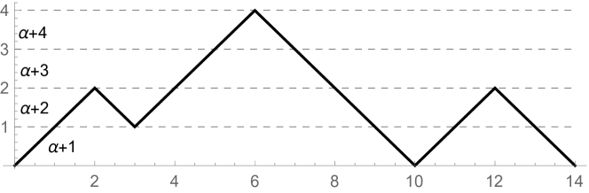
Figure 1: A Dyck path $p$ with weight $w(p)=(\alpha+1)^{2}(\alpha+2)^{3}(\alpha+3)(\alpha+4)$.

Let $\mathfrak{D}_{2n}^{*}$ be the set of all Dyck paths of length $2n$ which do not meet the $x$-axis except the starting and the ending points. Let

$$v_{n}(\alpha)=\sum_{p\in\mathfrak{D}^{*}_{2n}}w(p).$$

Since each Dyck path $p=(i_{0},i_{1},\dots,i_{2n-1},i_{2n})\in\mathfrak{D}_{2n}^{*}$ is one-to-one correspondence with a Dyck path $q=(i_{1}-1,i_{2}-1,\dots,i_{2n-1}-1)$ of length $2(n-1)$, it follows that

$$v_{n}(\alpha)=(\alpha+1)u_{n-1}(\alpha+1).$$

Moreover, let $2i$ be the first time that the Dyck path $p$ meets the $x$-axis. Then either $i=n$ or the Dyck path $p$ is the concatenation of a Dyck path in $\mathfrak{D}_{2i}^{*},(1\leq i<n),$ and another Dyck path of length $2(n-i)$. Thus,

$$u_{n}(\alpha) =v_{n}(\alpha)+\sum_{i=1}^{n-1}v_{i}(\alpha)u_{n-i}(\alpha)$$

$$=(\alpha+1)u_{n-1}(\alpha+1)+\sum_{i=1}^{n-1}(\alpha+1)u_{i-1}(\alpha+1)u_{n-i}(\alpha)$$

$$=(\alpha+1)\sum_{i=0}^{n-1}u_{i}(\alpha+1)u_{n-1-i}(\alpha).$$

The proof of (i) is complete. We will prove the second statement after the next lemma. ∎

Lemma 6.

Let $\alpha\geq 0$ be fixed. Let $\{a_{n}\}$ be a sequence defined recursively by

$$\begin{cases}a_{n}=(2n-1)a_{n-1}+\alpha\sum_{i=0}^{n-1}a_{i}a_{n-1-i},\quad n\geq 1,\\ a_{0}=1.\end{cases}$$ (6)

Let $\{b_{n}\}$ be a sequence defined by the following relations $b_{0}=1,$

$$a_{n}=(\alpha+1)\sum_{i=0}^{n-1}b_{i}a_{n-1-i},\quad n\geq 1.$$ (7)

Then $\{b_{n}\}$ satisfies an analogous recursive relation as $\{a_{n}\}$,

$$\begin{cases}b_{n}=(2n-1)b_{n-1}+(\alpha+1)\sum_{i=0}^{n-1}b_{i}b_{n-1-i},\quad n\geq 1,\\ b_{0}=1.\end{cases}$$ (8)

Proof.

Consider the field of formal Laurent series over ${\mathbb{R}}$, denoted by ${\mathbb{R}}((X))$,

$${\mathbb{R}}((X))=\left\{f(X)=\sum_{n\in{\mathbb{Z}}}c_{n}X^{n}:c_{n}\in{\mathbb{R}},c_{n}=0\text{ for }n<n_{0}\right\}.$$

The addition is defined as usual and the multiplication is well defined as

$$f(X)g(X)=\sum_{n\in{\mathbb{Z}}}\left(\sum_{i\in{\mathbb{Z}}}c_{i}d_{n-i}\right)X^{n},$$

for $f(X)=\sum c_{n}X^{n},g(X)=\sum d_{n}X^{n}\in{\mathbb{R}}((X))$. The quotient $f(X)/g(X)$ is understood as $f(X)g(X)^{-1}$ for $g(X)\neq 0$. The formal derivative is also defined as

$$f^{\prime}(X)=\sum_{n\in{\mathbb{Z}}}c_{n}nX^{n-1}\in{\mathbb{R}}((X)).$$

Now let

$$f(X)=\sum_{n=0}^{\infty}a_{n}X^{n},\quad g(X)=\sum_{n=0}^{\infty}b_{n}X^{n}.$$

It is straightforward to show that the recursive relation (6) is equivalent to the following equation

$$f(X)-1=2X^{2}f^{\prime}(X)+Xf(X)+\alpha Xf^{2}(X).$$

In addition, the relation (7) leads to

$$g(X)=\frac{f(X)-1}{(\alpha+1)Xf(X)}.$$

Finally, we can easily check that $g(X)$ satisfies

$$g(X)-1=2X^{2}g^{\prime}(X)+Xg(X)+(\alpha+1)Xg^{2}(X),$$

which is equivalent to the recursive relation (8). The proof is complete. ∎

Proof of Proposition 4(ii).

When $\alpha=0$, it is well known that $u_{n}(0)$ is the $2n$th moment of the standard Gaussian distribution, and is given by

$$u_{n}(0)=(2n-1)!!.$$

Consequently, the conditions in Lemma 6 are satisfied for $a_{n}=u_{n}(0),b_{n}=u_{n}(1)$ and $\alpha=0$. It follows that the recursive relation (5) then holds for $\alpha=1$. Continue this way, it follows that the recursive relation (5) holds for any $\alpha\in{\mathbb{N}}$. We conclude that it holds for all $\alpha$ because of the fact that $\{u_{n}(\alpha)\}$ is a polynomial of degree $n$ in $\alpha$. The proof is complete. ∎

3.3 Explicit formula for the spectral measure of $A_{\alpha}$, proof of Theorem 1(ii)

In this section, by using the method of Martin and Kearney [4], we derive the explicit formula for the mean spectral measure $\bar{\mu}_{\alpha}$ from the relation (5),

$$\begin{cases}u_{n}(\alpha)=(2n-1)u_{n-1}(\alpha)+\alpha\sum_{i=0}^{n-1}u_{i}(\alpha)u_{n-1-i}(\alpha),\quad n\geq 1,\\ u_{0}(\alpha)=1.\end{cases}$$

Recall that $u_{n}(\alpha)=\langle\bar{\mu}_{\alpha},x^{2n}\rangle$ and $\bar{\mu}_{\alpha}$ is a symmetric probability measure.

Let us extract here the main result of [4]. The problem is to find a function $\nu$ for which

$$\int_{0}^{\infty}x^{n-1}\nu(x)dx=u_{n},\quad n=1,2,\dots,$$

where the sequence $\{u_{n}\}$ is given by a general self-convolutive recurrence

$$\begin{cases}u_{n}=(\alpha_{1}n+\alpha_{2})u_{n-1}+\alpha_{3}\sum_{i=1}^{n-1}u_{i}u_{n-i},\quad n\geq 2,\\ u_{1}=1,\end{cases}$$ (9)

$\alpha_{1},\alpha_{2}$ and $\alpha_{3}$ being constants. Then the solution is given by (Eq. (13)–Eq. (16) in [4]),

$$\nu(x)=\frac{k(kx)^{-b}e^{-kx}}{\Gamma(a+1)\Gamma(a-b+1)}\frac{1}{U_{R}(kx)^{2}+U_{I}(kx)^{2}},$$

where,

$$U_{R}(x) =e^{-x}\bigg{(}\frac{\Gamma(1-b)}{\Gamma(a-b+1)}{}_{1}F_{1}(b-a;b;x)$$

$$\hskip 85.35826pt-(\cos\pi b)\frac{\Gamma(b-1)}{\Gamma(a)}x^{1-b}{}_{1}F_{1}(1-a;2-b;x)\bigg{)},$$

$$U_{I}(x) =(\sin\pi b)e^{-x}\frac{\Gamma(b-1)}{\Gamma(a)}x^{1-b}{}_{1}F_{1}(1-a;2-b;x),$$

and $k=1/\alpha_{1},a=\alpha_{3}/\alpha_{1},b=-1-\alpha_{2}/\alpha_{1}$, provided $\alpha_{1}\neq 0$. Here ${}_{1}F_{1}(a;b;z)$ is the Kummer function.

The sequence $\{u_{n}(\alpha)\}_{n\geq 0}$ is a particular case of the self-convolutive recurrence (9) with parameters $\alpha_{1}=2,\alpha_{2}=-3$ and $\alpha_{3}=\alpha$. Note that our sequence $\{u_{n}(\alpha)\}$ starts from $n=0$, and thus $\alpha_{2}=-3$. By direct calculation, we get $k=1/2,a=\alpha/2,$ and $b=1/2$. Therefore, the function $\nu_{\alpha}(x)$ for which $u_{n}(\alpha)=\int_{0}^{\infty}x^{n}d\nu_{\alpha}(x)dx,n=0,1,\dots,$ is given by

$$\nu_{\alpha}(x)=\frac{1}{\sqrt{2}\Gamma(\frac{\alpha}{2}+1)\Gamma(\frac{\alpha}{2}+\frac{1}{2})}\frac{1}{\sqrt{x}}e^{-\frac{x}{2}}\frac{1}{U_{R}(x/2)^{2}+U_{I}(x/2)^{2}},\quad x>0,$$

where

$$U_{R}(x) =e^{-x}\frac{\Gamma(\frac{1}{2})}{\Gamma(\frac{\alpha}{2}+\frac{1}{2})}{}_{1}F_{1}(\frac{1}{2}-\frac{\alpha}{2};\frac{1}{2};x),$$ (10)

$$U_{I}(x) =e^{-x}\frac{\Gamma(-\frac{1}{2})}{\Gamma(\frac{\alpha}{2})}x^{1/2}{}_{1}F_{1}(1-\frac{\alpha}{2};\frac{3}{2};x).$$ (11)

It is clear that $\nu_{\alpha}(x)>0$ for any $x>0$. Now it is easy to check that the function $\bar{\mu}_{\alpha}(y)$ defined by

$$\bar{\mu}_{\alpha}(y)=|y|\nu_{\alpha}(y^{2}),\quad y\in{\mathbb{R}},$$

satisfies the following relations

$$\int_{{\mathbb{R}}}y^{2n+1}\bar{\mu}_{\alpha}(y)dy=0,\quad\int_{{\mathbb{R}}}y^{2n}\bar{\mu}_{\alpha}(y)dy=u_{n}(\alpha),\quad n=0,1,\dots,$$

In other words, $\bar{\mu}_{\alpha}(y)$ is the density of the mean spectral measure $\bar{\mu}_{\alpha}$ with respect to the Lebesgue measure.

We are now in a position to simplify the explicit formula of $\bar{\mu}_{\alpha}$. Let

$$V_{R}(y) =\left(\frac{\Gamma(\frac{\alpha}{2}+1)\Gamma(\frac{\alpha}{2}+\frac{1}{2})}{\Gamma(\frac{1}{2})}\right)^{1/2}U_{R}(y^{2}/2),$$

$$=2^{-\frac{\alpha}{2}}\Gamma(\alpha+1)^{\frac{1}{2}}\frac{\Gamma(\frac{1}{2})}{\Gamma(\frac{\alpha}{2}+\frac{1}{2})}e^{-\frac{y^{2}}{2}}{}_{1}F_{1}(\frac{1}{2}-\frac{\alpha}{2};\frac{1}{2};\frac{y^{2}}{2}),$$

$$V_{I}(y) =-\left(\frac{\Gamma(\frac{\alpha}{2}+1)\Gamma(\frac{\alpha}{2}+\frac{1}{2})}{\Gamma(\frac{1}{2})}\right)^{1/2}U_{I}(y^{2}/2)$$

$$=-2^{-\frac{\alpha}{2}-\frac{1}{2}}\Gamma(\alpha+1)^{\frac{1}{2}}\frac{\Gamma(-\frac{1}{2})}{\Gamma(\frac{\alpha}{2})}{y}e^{-\frac{y^{2}}{2}}{}_{1}F_{1}(1-\frac{\alpha}{2};\frac{3}{2};\frac{y^{2}}{2}).$$

Here, in the above expressions, we have used the following relation for Gamma function

$$\frac{\Gamma(\frac{\alpha}{2}+\frac{1}{2})\Gamma(\frac{\alpha}{2}+1)}{\Gamma(\frac{1}{2})}=2^{-\alpha}\Gamma(\alpha+1).$$ (12)

Then $\bar{\mu}_{\alpha}(y)$ can be written as

$$\bar{\mu}_{\alpha}(y)=\frac{e^{-\frac{y^{2}}{2}}}{\sqrt{2\pi}}\frac{1}{V_{R}(y)^{2}+V_{I}(y)^{2}}.$$

Next, we will show that $V_{R}(y)$ and $V_{I}(y)$ are the Fourier cosine transform and Fourier sine transform of

$$f_{\alpha}(t)=\pi\sqrt{\frac{\alpha}{\Gamma(\alpha)}}t^{\alpha-1}\frac{e^{-\frac{t^{2}}{2}}}{\sqrt{2\pi}},$$

respectively. Let us now give definitions of Fourier transforms. The Fourier transform of a function $f\colon{\mathbb{R}}\to{\mathbb{C}}$ is defined to be

$${\mathcal{F}}(f)(y)=\frac{1}{\sqrt{2\pi}}\int_{-\infty}^{\infty}f(t)e^{iyt}dt,\quad(y\in{\mathbb{R}}),$$

and the Fourier cosine transform, the Fourier sine transform are defined to be

$${\mathcal{F}}_{c}(f)(y)=\sqrt{\frac{2}{\pi}}\int_{0}^{\infty}f(t)\cos(yt)dt,\quad(y>0),$$

$${\mathcal{F}}_{s}(f)(y)=\sqrt{\frac{2}{\pi}}\int_{0}^{\infty}f(t)\sin(yt)dt,\quad(y>0),$$

respectively. Then those transforms are related as follows

$$\begin{cases}{\mathcal{F}}(f)(y)={\mathcal{F}}_{c}(f)(y),\quad(y\geq 0),&\text{if $f(t)$ is even,}\\ {\mathcal{F}}(f)(y)=i{\mathcal{F}}_{s}(f)(y),\quad(y\geq 0),&\text{if $f(t)$ is odd.}\end{cases}$$

For $\alpha>0$, we have (cf. Formula 3.952(8) in [3])

$${\mathcal{F}}_{c}(t^{\alpha-1}e^{-\frac{t^{2}}{2}})=\frac{2^{\frac{\alpha}{2}-\frac{1}{2}}\Gamma(\frac{\alpha}{2})}{\sqrt{\pi}}e^{-\frac{y^{2}}{2}}{}_{1}F_{1}(\frac{1}{2}-\frac{\alpha}{2};\frac{1}{2};\frac{y^{2}}{2}).$$

Then by some simple calculations, we arrive at the following relation

$$V_{R}(y)={\mathcal{F}}_{c}(f_{\alpha}(t))(y),\quad y\geq 0.$$

Similarly,

$$V_{I}(y)={\mathcal{F}}_{s}(f_{\alpha}(t))(y),\quad y\geq 0,$$

by using Formula 3.952(7) in [3],

$${\mathcal{F}}_{s}(t^{\alpha-1}e^{-\frac{t^{2}}{2}})=\frac{2^{\frac{\alpha}{2}}\Gamma(\frac{\alpha}{2}+\frac{1}{2})}{\sqrt{\pi}}ye^{-\frac{y^{2}}{2}}{}_{1}F_{1}(1-\frac{\alpha}{2};\frac{3}{2};\frac{y^{2}}{2}).$$

By definitions, $V_{R}(y)$ is an even function and $V_{I}(y)$ is an odd function. Thus the following expression holds for all $y\in{\mathbb{R}}$,

$$V_{R}(y)+iV_{I}(y) =\sqrt{\frac{2}{\pi}}\int_{0}^{\infty}f_{\alpha}(t)(\cos(yt)+i\sin(yt)dt$$

$$=\sqrt{\frac{2}{\pi}}\int_{0}^{\infty}f_{\alpha}(t)e^{iyt}dt=:\hat{f}_{\alpha}(y).$$

Consequently,

$$V_{R}(y)^{2}+V_{I}(y)^{2}=|\hat{f}_{\alpha}(y)|^{2},$$

which completes the proof of Theorem 1(ii).

We plot the graph of the density $\bar{\mu}_{\alpha}(y)$ for several values $\alpha$ as in the following figure by using Mathematica. It follows from the Jacobi matrix form that the spectral measure of $\frac{1}{\sqrt{\alpha}}A_{\alpha}$ converges weakly to the semicircle law as $\alpha$ tends to infinity. Note that the semicircle law, the probability measure supported on $[-2,2]$ with the density

$$\frac{1}{2\pi}\sqrt{4-x^{2}},(-2\leq x\leq 2),$$

is the spectral measure of the following Jacobi matrix

$$\begin{pmatrix}0&1\\ 1&0&1\\ &1&0&1\\ &&\ddots&\ddots&\ddots\end{pmatrix}.$$

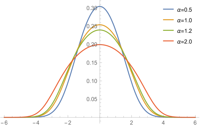
Figure 2: The density $\bar{\mu}_{\alpha}(y)$ for several values $\alpha$.

Remark 7.

When $\alpha$ in a positive integer number, we can give even more explicit expressions for $V_{R}(y)$ and $V_{I}(y)$.

• $\alpha=2n,n\in{\mathbb{N}}$. In this case, $f_{\alpha}(t)$ is an odd function. Therefore

  $$V_{I}(y)={\mathcal{F}}_{s}(f_{\alpha}(t))=-i{\mathcal{F}}(f_{\alpha}(t)).$$

  Note that

  $${\mathcal{F}}(e^{-\frac{t^{2}}{2}})=e^{-\frac{y^{2}}{2}}.$$

  Therefore, for integer $\alpha\geq 1$,

  $${\mathcal{F}}(t^{\alpha-1}e^{-\frac{t^{2}}{2}})=(i)^{\alpha-1}\frac{d^{\alpha-1}}{dy^{\alpha-1}}(e^{-\frac{y^{2}}{2}}).$$

  Consequently,

  $$V_{I}(y) =-i^{\alpha}\pi\sqrt{\frac{\alpha}{\Gamma(\alpha)}}\frac{d^{\alpha-1}}{dy^{\alpha-1}}(e^{-\frac{y^{2}}{2}})\frac{1}{\sqrt{2\pi}}$$

  $$=-i^{\alpha}\pi\sqrt{\frac{\alpha}{\Gamma(\alpha)}}e^{\frac{y^{2}}{2}}\frac{d^{\alpha-1}}{dy^{\alpha-1}}(e^{-\frac{y^{2}}{2}})\frac{e^{-\frac{y^{2}}{2}}}{\sqrt{2\pi}}$$

  $$=-i^{\alpha}\pi\sqrt{\frac{\alpha}{\Gamma(\alpha)}}He_{\alpha-1}\frac{e^{-\frac{y^{2}}{2}}}{\sqrt{2\pi}}.$$

  Here $He_{m}$ denotes probabilists’ Hermite polynomials.

• $\alpha=2n+1$. This case is very similar. Since $f_{\alpha}(t)$ is an even function, it follows that

  $$V_{R}(y)={\mathcal{F}}_{c}(f_{\alpha}(t))(y)={\mathcal{F}}(f_{\alpha}(t))=i^{\alpha-1}\pi\sqrt{\frac{\alpha}{\Gamma(\alpha)}}He_{\alpha-1}\frac{e^{-\frac{y^{2}}{2}}}{\sqrt{2\pi}}.$$

Trinh Khanh Duy

Institute of Mathematics for Industry

Kyushu University

Fukuoka 819-0395, Japan

e-mail: trinh@imi.kyushu-u.ac.jp

Tomoyuki Shirai

Institute of Mathematics for Industry

Kyushu University

Fukuoka 819-0395, Japan

e-mail: shirai@imi.kyushu-u.ac.jp

References

- [1] I. Dumitriu and A. Edelman: Matrix models for beta ensembles, J. Math. Phys. 43 (2002), no. 11, 5830–5847.
- [2] I. Dumitriu and A. Edelman: Global spectrum fluctuations for the -Hermite and -Laguerre ensembles via matrix models, J. Math. Phys. 47 (2006), no. 6, 063302, 36pp.
- [3] I.S. Gradshteyn and I.M. Ryzhik: Table of integrals, series, and products. Translated from the Russian. Translation edited and with a preface by Alan Jeffrey and Daniel Zwillinger. With one CD-ROM (Windows, Macintosh and UNIX). Seventh edition. Elsevier/Academic Press, Amsterdam, 2007.
- [4] R.J. Martin and M.J. Kearney: An exactly solvable self-convolutive recurrence, Aequationes Math. 80 (2010), no. 3, 291–318.
- [5] OEIS, the On-line Encyclopedia of Integer Sequences. https://oeis.org/
- [6] B. Simon: Szegö’s theorem and its descendants. Spectral theory for perturbations of orthogonal polynomials. M. B. Porter Lectures. Princeton University Press, Princeton, NJ, 2011.
- [7] N.S. Witte and P.J. Forrester: Moments of the Gaussian ensembles and the large- expansion of the densities, J. Math. Phys. 55 (2014), 083302 .