Simulations to study the static polarization limit for RHIC lattice with the Polymorphic Tracking Code

Abstract

We report a study of spin dynamics based on simulations with the Polymorphic Tracking Code (PTC), exploring the dependence of the static polarization limit on various beam parameters and lattice settings for a practical RHIC lattice.

Introduction

The motion of the spin expectation value (the “spin”) $\vec{S}$ of a charged particle traveling in the electric and magnetic fields in a circular accelerator is described by the Thomas-BMT equation L.H.Thomas1927 , ${d\vec{S}}/{d\theta}=\vec{\Omega}(\vec{z},\theta)\times\vec{S}$, where $\theta$ is the azimuthal angle, $\vec{z}$ is the location in the 6-dimensional (6D) phase space and $\vec{\Omega}$ contains the electric and magnetic fields in the laboratory frame. For calculations it is convenient to write $\vec{\Omega}(\vec{z},\theta)={\vec{\Omega}}_{0}(\theta)+\vec{\omega}(\vec{z},\theta)$ where ${\vec{\Omega}}_{0}(\theta)$ is the contribution from motion on the closed orbit and $\vec{\omega}(\vec{z},\theta)$ is the contribution from the synchro-betatron motion.

It is often necessary to describe spin motion with the help of a unit vector field ${\hat{n}}(z,\theta)$ (the ”invariant spin field”, or ISF for short) D.P.Barber2004 and this object will play a central rôle in this paper. This satisfies the Thomas-BMT equation along particle trajectories and is periodic with respect to $\theta$: $\vec{n}(\vec{z},\theta+2\pi)=\vec{n}(\vec{z},\theta)$. The product $J_{s}=\vec{S}\cdot\vec{n}$ is an invariant of motion, and the motion of $\vec{S}$ is simply a precession around the local $\vec{n}$-axis. The spin precession frequency around $\hat{n}$ is characterized by the amplitude dependent spin tune $\nu_{s}$ D.P.Barber2004 . Let us assume that the 6D orbital motion is integrable and away from orbital resonances and spin-orbit resonances (defined below). Then the static polarization limit Vogt $P_{\text{lim}}=|\langle\vec{n}(\vec{z},\theta)\rangle|$, with the inner average taken over orbital phases, is the maximum achievable equilibrium beam polarization on a phase-space torus. On the closed orbit, $\vec{n}$ is denoted by $\vec{n}_{0}$ and it is normally vertical in the arcs and $\nu_{s}$ reduces to the closed orbit spin tune $\nu_{0}$. In a perfectly aligned planar ring, $\nu_{0}=G\gamma_{0}$, where $G=1.79284739$ for protons, and $\gamma_{0}$ is the relativistic factor for the design energy. The $\vec{n}$-axis diverges from $\vec{n}_{0}$ near the following spin-orbit resonances (or “spin resonances” in short), and $P_{\text{lim}}$ can be small,

$$\nu_{s}=k+k_{x}\nu_{x}+k_{y}\nu_{y}+k_{z}\nu_{z},~{}~{}~{}k,~{}k_{x},~{}k_{y},~{}k_{z}\in\mathbb{Z}.$$ (1)

Note that $\nu_{s}$ is usually undefined on orbital resonances, otherwise $\nu_{s}$ is only a function of the orbital actions $\vec{J}$ and the optical state of the ring. In particular, if $\nu_{s}(\vec{J})$ is an amplitude dependent spin tune, then the fractional part of $\pm\nu_{s}(\vec{J})+l_{0}+\vec{l}\cdot\vec{\nu}$, with $l_{0}\in\mathbb{Z}$ and $\vec{l}\in\mathbb{Z}^{3}$ is also an amplitude dependent spin tune. In other words, there is an equivalence class of amplitude dependent spin tunes D.P.Barber2004 . In addition, the dip in $P_{\text{lim}}$ across a spin resonance is accompanied by a jump in the amplitude dependent spin tune so that a system can never actually sit at a resonance as defined in Eq. (1) Vogt ; Hoffstaetter:2004ra . The order of a resonance is defined as $|k_{x}|+|k_{y}|+|k_{z}|$. Normally $\nu_{s}$ stays close to $\nu_{0}$.

In a planar ring, the most important spin resonances are those due to vertical closed orbit distortions, which occur near $\nu_{0}=k,~{}k\in\mathbb{Z}$, namely the imperfection spin resonances; and those driven by the vertical betatron oscillations, which occur near $\nu_{0}=k\pm\nu_{y},~{}k\in\mathbb{Z}$, namely the first order intrinsic spin resonances with $|k_{y}|=1$. The major challenge in a high energy polarized proton synchrotron like RHIC is to preserve the beam polarization during acceleration RHICPPCMan ; prl_205GeV . The well-known Frossart-Stora formula Froissart-Stora describes the polarization loss after crossing a single isolated spin resonance. Introduction of a pair of diametrically opposed orthogonal Siberian snakes Derbenev1978 renders the closed orbit spin tune to be $\nu_{0}=0.5$ and independent of the beam energy. Therefore intrinsic resonances are avoided for normal $\nu_{y}$ during acceleration and even with misalignments, $\nu_{0}$ remains close to $0.5$ independently of the energy so that imperfection resonances are avoided too. However, at rational vertical tunes satisfying the condition $1/2+k=m\nu_{y},~{}m,k\in\mathbb{Z}$, there still can be strong loss of polarization during acceleration. This phenomeon is traditionally called “snake resonance” S.Y.Lee1986 ; S.Y.Lee1997 although for rational $\nu_{y}$ the amplitude dependent spin tune does not exist so that this condition does not correspond to higher-order resonance as defined in Eq. 1 . Of course in a real ring with misalignments, $\nu_{0}$ need not be exactly 0.5. Then pairs of real resonances in the sense of Eq. 1 with irrational $\nu_{y}$ can appear, sitting symmetrically on each side of the $\nu_{y}$ for the “snake resonance”. These doublets can also cause loss of polarization during acceleration.

Inspired by the Froissart-Stora formula, in rings without snakes, it is common practice to compute the strengths of the imperfection and intrinsic resonances for a practical lattice, and identify the most dangerous ones. Near one of these dangerous spin resonances, one can invoke the so-called “single resonance model” Courant1980 ; S.R.Mane1988 . This model is based on the rotating wave approximation whereby the effect of $\vec{\omega}$ is dominated by one particular Fourier harmonic at $\kappa=k+k_{x}\nu_{x}+k_{y}\nu_{y}+k_{z}\nu_{z},~{}k,k_{x},k_{y},k_{z}\in\mathbb{Z}$, with $|k_{x}|+|k_{y}|+|k_{z}|\leq 1$, and the corresponding resonance strength is $\epsilon_{\kappa}$. This lattice-independent model is analytically solvable, and can be extended to include Siberian snakes, often modeled by “point-like” spin rotations. These lattice-independent models have been extensively studied for proton storage rings. Analytical solutions for ${\nu_{s}}$ S.R.Mane2008 and the $\vec{n}$-axis S.R.Mane2002b ; S.R.Mane2003 ; S.R.Mane2008 have been obtained, as well as $P_{\text{lim}}$ S.R.Mane2004 . Thus as in Ref. S.R.Mane2008 , $\nu_{s}$ is 0.5 independently of the betatron amplitude, if $\nu_{y}$ is irrational. Moreover, as shown in Barber2003 ; Barber2006 simulations with these lattice-independent models are a great help for understanding the peculiar features of spin dynamics for rational $\nu_{y}$ and, in particular, on and near “snake resonances”.

However, in high-energy proton rings, the basic spin resonances (i.e., without snakes) of interest might not be well isolated, then a lattice-dependent study is necessary. For example, as we explain in Sections II.1 and  II.2 below, doublets of higher-order resonances at irrational $\nu_{y}$ can occur near to the $\nu_{y}$ of a “snake resonance” since $\nu_{s}$ need not be 0.5.

An extensive lattice-dependent study of the behavior of $P_{\text{lim}}$ throughout the whole energy range was made in the study of polarized proton beams up to 920 GeV in HERA Vogt ; G.H.Hoffstaetter2006 , as an approach complementary to direct spin tracking for acceleration. It is also interesting to study $P_{\text{lim}}$ for the store conditions of RHIC, with a beam energy of 255GeV, since this is relevant for the study of polarization variation during physics stores with constant beam energy V.Schoefer2012 ; Spin2014 .

In section I, methods for modeling and simulation based on the Polymorphic Tracking Code (PTC) are described, and in section II the results of the simulation are presented.

I The model for the simulations and the methods

The simulations in this paper utilize the Polymorphic Tracking Code (PTC) developed by E. Forest Schmidt:2002vp . Designed to model various geometries of particle accelerators, PTC is capable of symplectic tracking of the orbital motion and length-preserving transport of spin S.Mane2009PTC , where vectors of particle coordinates and Taylor maps can be tracked in a polymorphic manner, and where the latter enables the normal form analysis of the one-turn map using FPP fppipac2006 . Fortran programs have been developed to do the spin tracking, which call PTC as a library. The modeling of the RHIC lattice is presented first, followed by an explanation of the methods of simulation.

I.1 Modeling of the RHIC lattice

The MADX model of the RHIC lattice is exported into an input file for PTC, which is read by the Fortran program. When a particle is tracked through an integration step of a magnet body, the orbital transfer map is sandwiched in between two spin kicks in equal amounts and each orbital transfer map is a second-order symplectic integrator while each spin kick is represented by a $3\times 3$ orthogonal rotation matrix. The quadrupoles must be split into many integration steps to ensure the accuracy of orbital and spin tracking. An upper limit is set for the spin rotation angle of each integration step, calculated for the betatron amplitude of the tracked particle. In this study, we use about 7 integration steps for each arc quadrupole, and up to 81 integration steps for the quadrupoles in the final focus triplets.

There are two different implementations of a Siberian snake in this study. The first method implements a zero length spin kick that rotates a spin by 180 degrees around an axis in the lattice, namely a “point-like snake”, while the second method implements helical dipoles HelicalDipole into the lattice, namely a “helical dipole snake”. In PTC, a helical dipole is modeled with a symplectic transfer map accurate to the 4-th order. Note that the longitudinal magnetic field inside helical dipoles will introduce a small transverse coupling at large orbital excursions.

This study implements a pair of diametrically opposed snakes and therefore the closed-orbit spin tune is 0.5. Note that the spin rotators around IP6 (interaction point at 6 o’clock) and IP8 (interaction point at 8 o’clock) are not included in this study, but they can also be modeled in a similar way.

The beam-beam interaction is the major beam-current-dependent effect that might affect the beam polarization during physics stores. The effect of the beam-beam interaction on the beam polarization was studied through long-term tracking, with a lattice-independent model Batygin and element-by-element tracking Lucio1997 , where the beam-beam kick on spin motion was taken into account. However, the total beam-beam parameter Hirata from the two IPs in RHIC is within -0.015, and the contribution from the linearized beam-beam kick to the intrinsic resonance strength, is less than that of an arc quadrupole Lucio1997 . Therefore, the beam-beam spin kick is not too important. Nevertheless, the beam-beam interaction also introduces an incoherent tune shift for beam particles. This effect is studied in this work, with a thin-lens weak-strong beam-beam kick implemented for the orbital motion.

I.2 Simulation method

The $\vec{n}$-axis is calculated in PTC using stroboscopic averaging K.Heinemann1996 . Once $\vec{n}$ is computed for a phase space point $\vec{z}$ at an azimuth $\theta$, a particle is launched at the same location with spin parallel to $\vec{n}$ and tracked for $5000$ turns. If none of the three orbital tunes is rational, then the turn-by-turn orbital coordinates trace phase space points on the same torus, and the turn-by-turn spins $\{\vec{S}^{\parallel}_{j}\},j=1,2{\cdots}5000$ are the local $\vec{n}$ at the corresponding phase space points. Therefore, $P_{\text{lim}}$ can be calculated as an average over $\{\vec{S}^{\parallel}_{j}\}$ for such a phase space torus. In addition, the amplitude dependent spin tune can be obtained by a Fourier analysis of the spin motion according to Ref. D.P.Barber2004 . So a particle is launched with its spin perpendicular to $\vec{n}$, and tracked for $5000$ turns, and a turn-by-turn spin series $\{\vec{S}^{\bot}_{j}\}$ is obtained. The NAFF algorithm Laskar is then applied to calculate the fundamental frequency of the complex series $\{S^{\bot}_{xj}+iS^{\bot}_{zj}\}$, i.e., the amplitude dependent spin tune, in the range $[0.4,0.5]$.

II Simulation of RHIC polarization at store

In this section, the dependence of $P_{\text{lim}}$ on various beam parameters is studied for the Run 12 baseline lattice of the RHIC Blue ring, during physics stores. The default working point is $\nu_{x}/\nu_{y}=28.695/29.685$, and $\beta_{x}/\beta_{y}=0.62\text{m}/0.64\text{m}$ at the two interaction points IP6 and IP8 where the detectors STAR and PHENIX are located, respectively. the chromaticities are corrected to $\xi_{x}/\xi_{y}=1.85/2.27$ with two families of arc sextupoles. $\vec{n}$ and $P_{\text{lim}}$ are calculated at IP6, while $\nu_{s}$ is independent of the azimuthal angle. The betatron amplitudes are normalized with the amplitude corresponding to a normalized 95% emittance of $10\pi\text{mm}\cdot\text{mrad}$. Two cases with two different beam energies are simulated, and the relevant parameters are shown in Table. 1. Note that Case 1 is the beam energy of physics data taking, while Case 2 corresponds to the beam energy of a very strong intrinsic resonance around $[\nu_{y}]=0.7$ during the energy ramp.

Parameter	Case 1	Case 2
Beam energy(GeV)	254.8675	200.6022
$G\gamma_{0}$	487	383.31
Normalized 95% emittance($\pi~{}\text{mm}\cdot\text{mrad}$)	10.0	10.0
Intrinsic resonance strength	0.0026/0.0013	0.175

Table 1: Parameters of the RHIC lattice used in scans of $P_{\text{lim}}$

II.1 Amplitude scan

For a fixed lattice, different betatron amplitudes contribute to different underlying spin resonance strengths. Therefore they will lead to different behaviors of the $\vec{n}$-axis on the tori and different values of $P_{\text{lim}}$. In this study, a scan of $P_{\text{lim}}$ and $\nu_{s}$ over different vertical betatron amplitudes is investigated for Case 1 and Case 2, while the synchrotron amplitude is set to zero. Note that for the cases with helical dipole snakes, the snakes introduce a small transverse coupling so that there is a nonzero but small horizontal betatron amplitude.

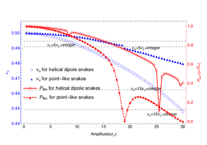
(a) Case 1

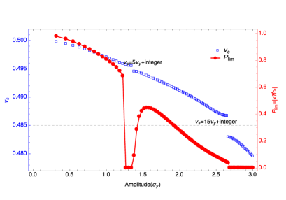
(b) Case 2

Figure 1: (color online) $P_{\text{lim}}$ and $\nu_{s}$ versus vertical amplitudes for Cases 1 and 2. Here, the range of vertical betatron amplitudes is ten times larger in Case 1 than that in Case 2. The betatron amplitudes are normalized by 10$\pi~{}\text{mm}\cdot\text{mrad}$. The fractional vertical betatron tune near the closed orbit is set to 0.699. The helical dipole snakes are implemented for both cases, while the point-like snakes are also implemented for Case 1. In addition, the locations of visible higher order spin resonances are indicated as the intersections between the horizontal dashed lines and the $\nu_{s}$ curves in the plots. Note that there are two resonances of the form $\nu_{s}=15\nu_{y}+\text{integer}$ in Case 1, due to the variation of $\nu_{y}$ with such large vertical betatron amplitudes.

In Fig. 1, the behavior of $P_{\text{lim}}$ and $\nu_{s}$ is compared between Case 1 and Case 2, and between different snake implementations. $P_{\text{lim}}$ in general becomes smaller with increasing vertical betatron amplitude, and has dips near spin resonances. Note that the range of vertical betatron amplitudes in Case 1 is 10 times larger than that in Case 2, and $P_{\text{lim}}$ decreases with amplitude much slower in Case 1 than Case 2, with a much smaller underlying intrinsic resonance strength. In the lattice-independent model with a single vertical resonance driving term and two diametrically opposed orthogonal Siberian snakes, it was shown Barber2003 ; S.R.Mane2008 that $\nu_{s}$ is 0.5 independently of the betatron amplitude, if the fractional betatron tune is irrational. However, when the betatron amplitude becomes larger in the real lattice, the nearby spin resonances are no longer isolated in both cases, and this analytical model is violated. Then we find that $\nu_{s}$ is shifted away from 0.5 with amplitude, due to interference between nearby spin resonances. Note that the shift of $\nu_{s}$ from 0.5 is in general much larger in Case 2 than Case 1 for the same betatron amplitude. Moreover, the locations of the spin resonances $5\nu_{y}-\nu_{s}=\text{integer}$ are indicated in the plots and match the sudden dips of $P_{\text{lim}}$ and the jump of $\nu_{s}$. Several other higher order spin resonances are also visible and indicated in the plot, and big jumps correlate with wide resonances. In Case 1, the betatron amplitude becomes so large that the amplitude dependent orbital tune shift is not negligible, and there are two locations corresponding to the same kind of spin resonance $\nu_{s}=15\nu_{y}+\text{integer}$. In addition, in Case 1, except for the location of spin resonances, $P_{\text{lim}}$ decreases faster with amplitude for the point-like snakes, while $\nu_{s}$ shifts faster away from $0.5$ with amplitude for the helical dipole snakes, and the spin resonance $\nu_{s}=5\nu_{y}+\text{integer}$ is wider for the point-like snakes. Because the helical dipoles also contribute to the driving term of the spin resonances, for this case, it appears that the contribution from the helical dipoles cancels part of the total resonance strength mainly driven by the quadrupoles.

II.2 Betatron tune scan

For a fixed vertical betatron amplitude, different vertical betatron tunes correspond to different distances from major spin resonances. Therefore they will lead to different values of $P_{\text{lim}}$ at the same vertical betatron amplitude. In this section, the integer part of betatron tunes are kept constant so that “vertical betatron tune” refers to the fractional vertical betatron tune. A list of vertical betatron tunes in a selected range is generated with a fixed step size, and the lattice is then fitted accordingly for each case with a fixed fractional horizontal tune $\nu_{x}=0.69$. $P_{\text{lim}}$ is computed for these lattice settings with the same vertical betatron amplitude 10$\pi~{}\text{mm}\cdot\text{mrad}$. Helical dipole snakes are used in this simulation.

Fig. 2 is a scan in the range $\nu_{y}\in[0.501,0.98]$ with a step size of 0.0005.

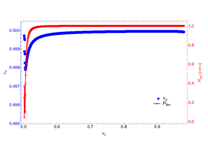
(a) Case 1

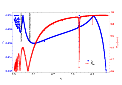
(b) Case 2

Figure 2: (color online) $P_{\text{lim}}$ versus fractional vertical betatron tune in the range $[\nu_{y}]\in[0.501,0.980]$. For both cases, the step size of tune scan is 0.0005. The vertical normalized emittance is 10$\pi~{}\text{mm}\cdot\text{mrad}$, and the horizontal tune is set to 0.69. Helical dipole snakes are implemented in both cases. Two locations of “nonresonant beam polarization” are indicated in Case 2.

It is clearly seen that in Case 2, $P_{\text{lim}}$ is generally smaller when $\nu_{y}$ is closer to $0.5$, which indicates that the spin resonance $\nu_{s}=\nu_{y}+\text{integer}$ is so strong that it affects the behavior of $P_{\text{lim}}$ in the whole scan range. In Case 1, however, the strength of the resonance $\nu_{s}=\nu_{y}+\text{integer}$ appears to be much smaller. Moreover, several other higher order spin resonances are also visible in Case 2, indicating that their widths are comparable or larger than the step size $0.0005$ in the vertical tune dimension. Several locations of “non-resonant beam depolarization” are also observed in this plot, where the the dips in $P_{\text{lim}}$ do not correspond to a jump in $\nu_{s}$, i.e., the locations of spin resonances. As shown in Ref. S.R.Mane2004 , for the lattice-independent model with an isolated vertical resonance driving term and two diametrically opposed orthogonal snakes, $P_{\text{lim}}$ can be analytically expressed via a special function $a_{0}$ of the resonance strength, betatron tune and $G\gamma_{0}$, which goes to zero at the locations of “non-resonant beam depolarization” of that model. This is an example where the study of these lattice-independent models leads to physical insights that are nontrivial to obtain otherwise.

The vertical betatron tune range $[0.67,0.74]$ is of particular interests because the vertical tunes of current RHIC operations are in this range. The scan result with a step size $0.0001$ is shown in Fig. 3, where helical dipole snakes are applied.

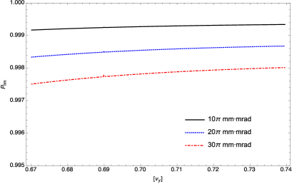
(a) Case 1

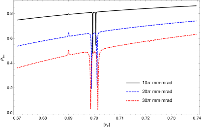
(b) Case 2

Figure 3: (color online) $P_{\text{lim}}$ versus fractional vertical betatron tune in the range of $[\nu_{y}]\in[0.67,0.74]$ for both cases, the step size of the tune scan is 0.0001. Three different vertical amplitudes are shown for Case 1 and Case 2. The horizontal tune is set to 0.69. Helical dipole snakes are implemented in both cases.

In Case 2, with this step size, it is clear that the 7/10 “snake resonance” is split into a doublet, due to the fact that $\nu_{s}$ shifts with $\nu_{y}$. So the locations of the double resonances shift with amplitude as well, while the widths of these spin resonances increase with amplitude. Due to the transverse coupling introduced by the helical dipoles, there is a small blip in $P_{\text{lim}}$ at $\nu_{y}=\nu_{x}=0.69$, which is not visible if point-like snakes are used instead. However, in Case 1, the widths of the spin resonances are very small and invisible in the plot. Moreover, except for the resonance locations, it is shown that $P_{\text{lim}}$ increases with the vertical tune in this tune range.

II.3 Effect of the beam-beam interaction

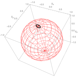
(a) The $\vec{n}$-axis on one phase space torus.

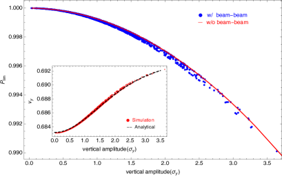
(b) $P_{\text{lim}}$ and $\nu_{y}$ versus vertical amplitude

Figure 4: (color online) The effect of beam-beam interaction on $P_{\text{lim}}$. The left plot shows the turn-by-turn $\vec{n}$-axis of one tracked particle. The right plot shows $P_{\text{lim}}$ versus vertical amplitude for the cases with or without beam-beam interaction. In addition, the betatron tunes of tracked particles (“Simulation”) are compared with the analytical amplitude dependence of the tune shifts (“Analytical”) Hirata , in the presence of the beam-beam interaction. This is shown in the small figure inside the right plot. 1008 particles with a Gaussian distribution were launched in the tracking. The beam-beam parameter is $-0.012$, and the fractional tunes are (0.690, 0.695).

A thin-lens weak-strong beam-beam kick to the vertical betatron motion, is implemented at IP6, with a vertical beam-beam parameter of $-0.012$. A beam of 1008 particles, with a Gaussian distribution for the vertical coordinates is launched and the $P_{\text{lim}}$ is computed for each particle’s trajectory(torus). As shown in Fig 4, the calculated turn-by-turn $\vec{n}$-axis of one particle forms a closed curve on the surface of a unit sphere, and this indicates the existence of an $\vec{n}$-axis on the particle’s torus in the presence of nonlinear betatron motion. Moreover, the effect of beam-beam interaction on $P_{\text{lim}}$ is insignificant. Note that the helical dipole snakes introduce a small transverse coupling in this example.

II.4 Effect of horizontal motion

The simulations for the cases shown above deal primarily with the vertical betatron motion, since the contribution of the small horizontal amplitude introduced by the helical dipoles is small for these cases. We now include horizontal motion by initializing a beam with a 4D Gaussian distribution. The normalized 95% emittances are 10$\pi~{}\text{mm}\cdot\text{mrad}$ for both horizontal and vertical planes. Two cases are simulated as shown in Fig. 5, one without beam-beam interaction, and the other with a beam-beam kick at IP6, whose beam-beam parameter is -0.012. Compared to the case with only vertical betatron motion, when 4D motion is included, $P_{\text{lim}}$ spreads out with vertical amplitude to some extent, for different trajectories. However, the two cases with or without beam-beam effect do not show much difference. This is because the variation of $P_{\text{lim}}$ with vertical betatron tune is very small for Case 1 in the tune range between 0.67 and 0.74, as shown in Fig. 3.

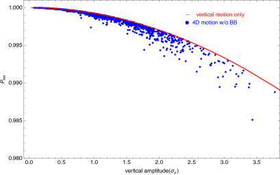
(a) 4D motion without beam-beam interaction

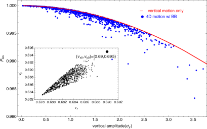
(b) 4D motion with beam-beam interaction

Figure 5: (color online) Comparison of $P_{\text{lim}}$ versus vertical betatron amplitude, as normalized by $10\pi\text{mm}\cdot\text{mrad}$ for 1008 trajectories, between the case with 4D motion, and the case with only vertical betatron motion. The left plot shows the case without beam-beam interaction, and the right plot shows the case with beam-beam interaction. The 95% normalized emittances are 10$\pi~{}\text{mm}\cdot\text{mrad}$ for both horizontal and vertical planes. A beam-beam kick with a beam-beam parameter -0.012 is implemented at IP6 of the RHIC lattice, for the right plot, and the tune footprint of the beam particles is shown in a small figure inside the right plot as well. The fractional tunes are set to $(0.69,0.695)$.

III Conclusion

In this paper we compute the static polarization limit for a practical RHIC lattice with the physics store conditions for various beam parameters, as a step towards understanding the polarization evolution at store. All calculations are done on the basis of the Polymorphic Tracking Code. It is shown that the vertical betatron oscillation has the dominant effect on the behavior of the $P_{\text{lim}}$ in contrast with the horizontal oscillations. Note that synchrotron motion is not included in this simulation because the synchrotron tune of RHIC is very small, namely around $3\times 10^{-4}$ at store. In this case the use of stroboscopic averaging to find the $\vec{n}$-axis when synchrotron motion is included requires special studies. Moreover, the practical modeling of Siberian snakes with helical dipoles leads to different behavior of $P_{\text{lim}}$ and $\nu_{s}$, in contrast to the implementation of the point-like Siberian snakes. So it is advisable to model the snakes carefully. The “nonresonant beam polarization” observed and studied in the lattice-independent model is also observed in this lattice-dependent model. Moreover, the beam-beam interaction doesn’t have much effect on $P_{\text{lim}}$ for the parameters under study. In addition, machine imperfections can possibly tilt $\vec{n}_{0}$ from the vertical and thereby lead to spin resonances due to horizontal motion. Imperfections can also shift $\nu_{0}$ away from 0.5 Ptitsyn:2010zz . A realistic treatment of various sources of machine imperfections requires a very careful lattice modeling, and is beyond the scope of this paper. Nevertheless, this work shows how a study of $P_{\text{lim}}$ and $\nu_{s}$ can give insights at fixed energies that are not available by executing simple tracking.

This work is supported under Contract No. DE-AC02-98CH10886 with the U.S. Department of Energy, the Hundred-Talent Program (Chinese Academy of Sciences), and National Natural Science Foundation of China (11105164). We would like to thank Drs. D. Abell and E. Forest on their help with the simulation code PTC, Drs. M. Bai, D. P. Barber, F. Meot, Y. Luo, V. Ptitsyn, V. Ranjbar and T. Roser for helpful discussions. One of us, Z. Duan, would like to thank Prof. M. Bai for being his host during his stay in BNL, guiding him into this field and the many instructive discussions over the years. He also would like to thank Dr D. P. Barber for helpful suggestions and discussions and careful reading of the manuscript. The simulation work used the resources of the National Energy Research Scientific Computing Center, a DOE Office of Science User Facility supported by the Office of Science of the U.S. Department of Energy under Contract No. DE-AC02-05CH11231.

References

- (1) L. H. Thomas, Phil. Mag. 3 (1927) 1-21; V. Bargmann, L. Michel, V. L. Telegdi, Phys. Rev. Lett. 2 (1959) 435.
- (2) D. P. Barber, J. Ellison, K. Heinemann, Phys.Rev. ST Accel.Beams 7 (2004) 124002.
- (3) M. Vogt, Doctorate Thesis, University of Hamburg, Report DESY-THESIS-2000-054 (2000).
- (4) G. H. Hoffstaetter and M. Vogt, Phys. Rev. E 70, 056501 (2004)
- (5) I. Alexseev et al., Design Manual - Polarized proton Collider at RHIC, BNL (1998).
- (6) M. Bai el al., Phys. Rev. Lett. 96, 174801 (2006).
- (7) M. Froissart and R. Stora, Nucl. Instrum. Meth. 7 (1960) 297.
- (8) Y. Derbenev, A. Kondratenko, Part. Accel. 8 (1978) 115.
- (9) S. Y. Lee and S. Tepikian, Phys. Rev. Lett. 56 (1986) 1635.
- (10) S. Y. Lee, “Spin Dynamics and Snakes in Synchrotrons”, World Scientific, Singapore, 1997.
- (11) E. D. Courant and R. D. Ruth, BNL Report 51270, BNL, 1980.
- (12) S. R. Mane, FNAL Report TM-1515, FNAL, 1988.
- (13) S. R. Mane, Nucl. Instrum. Meth. A 587 (2008) 188.
- (14) S. R. Mane, Nucl. Instrum. Meth. A 485 (2002) 277.
- (15) S. R. Mane, Nucl. Instrum. Meth. A 498 (2003) 1.
- (16) S. R. Mane, Nucl. Instrum. Meth. A 528, 677 (2004).
- (17) D. P. Barber, R. Jaganathan and M. Vogt, in: Proc. 15th Int. Spin Physics Symposium, Long Island, USA, 2002. and arXiv:physics/0502121 [physics.acc-ph].
- (18) D. P. Barber and M. Vogt, New J. Phys. 8 (2006) 296.
- (19) G. H. Hoffstaetter, “High-energy polarized proton beams: A modern view. Springer Tracts in Modern Physics”, Volumn 218, Springer, 2006.
- (20) V. Schoefer, et al., in: Proc. IPAC2012, New Orleans, USA, 2012; for the measured store polarization deterioration data in RHIC fills, refer to the RHIC spin group website: https://wiki.bnl.gov/rhicspin/RHIC_Spin_Group.
- (21) Z. Duan, M. Bai, T. Roser and Q. Qin, in: Proc. 21th Int. Spin Physics Symposium, Beijing, China, 2014.
- (22) F. Schmidt, E. Forest, E. McIntosh, CERN-SL-2002-044-AP, KEK-REPORT-2002-3 (2002).
- (23) S. Mane, KEK Report KEK-2009-8, KEK (2009).
- (24) E. Forest, Y. Nogiwa, in: Proc. ICAP 2006, Chamonix, France, 2006.
- (25) V. I. Ptitsyn and Y. M. Shatunov, in: Proc. Third Workshop on Siberian Snakes and Spin Rotators (A. Luccio and Th. Roser Eds.) NY, USA, 1994, Brookhaven National Laboratory Report BNL-52453, p.15.
- (26) Y. K. Batygin and T. Katayama, Phys. Rev. E 58 (1998) 1019.
- (27) A. Luccio and M. Syphers, BNL report AGS/RHIC/SN-068, BNL (1997).
- (28) K. Hirata, Handbook of accelerator physics and engineering, edited by A. W. Chao, K. H. Mess, M. Tigner and F. Zimmermann, 2nd edition, 1st printing, World Scientific (2013).
- (29) K. Heinemann and G. H. Hoffstätter, Physical Review E 54 (1996) 4240.
- (30) J. Laskar, C. Froeschlé and A. Celletti, Physica D, 56, (1992) 253.
- (31) V. Ptitsyn, M. Bai and T. Roser, in: Proc. IPAC 2010, Kyoto, Japan, 2010.