SKA Pathfinders Radio Continuum Surveys 2015 - SPARCS

Multi-frequency image reconstruction
for radio interferometry.
A regularized inverse problem approach.

Abstract.

We describe a “spatio-spectral” deconvolution algorithm for wide-band imaging in radio interferometry. In contrast with the existing multi-frequency reconstruction algorithms, the proposed method does not rely on a model of the sky-brightness spectral distribution. This non-parametric approach can be of particular interest for the new generation of low frequency radiotelescopes. The proposed solution formalizes the reconstruction problem as a convex optimization problem with spatial and spectral regularizations. The efficiency of this approach has been already proven for narrow-band image reconstruction and the present contribution can be considered as its extension to the multi-frequency case. Because the number of frequency bands multiplies the size of the inverse problem, particular attention is devoted to the derivation of an iterative large scale optimization algorithm. It is shown that the main computational bottleneck of the approach, which lies in the resolution of a linear system, can be efficiently overcome by a fully parallel implementation w.r.t. the frequencies, where each processor reconstructs a narrow-band image. All the other optimization steps are extremely fast. A parallel implementation of the algorithm in Julia is publicly available at https://github.com/andferrari. Preliminary simulations illustrate the performances of the method and its ability to reconstruct complex spatio-spectral structures.

1. Introduction

Recently, much attention has been paid to the development of image reconstruction algorithms for the incoming and future radio facilities. Most recent contributions, such as (Carrillo et al., 2012; Dabbech et al., 2015; Carrillo et al., 2014) or (Garsden et al., 2015) heavily rely on sparse estimation. In the wake of CLEAN algorithm (Högbom, 1974) and its multiresolution variants, sparse models have indeed proved in the last decades to be a powerfull approach for radiointerferometric image reconstruction in particular, and for the resolution of inverse problems in general.

In addition to their high spatial resolution, the wide bandwidths of the new generation of radio interferometers makes possible the reconstruction of complex spectral structures. The Square Kilometre Array (SKA) and its precursors will achieve (sub-)arcsec resolution over hundreds of MHz instantaneous bandwidths and with a tremendously broad band coverage (see Table 1 in the SKA1 System Baseline Design document (Dewdney et al., 2013)). The reconstruction of both spatial and spectral behaviour of continuum radio sources is an essential tool to characterize the astrophysical origin of their detected radiation, e.g. (Kraus, 1986). (Rau and Cornwell, 2011) opened the way to multi-frequency deconvolution algorithms, which aim to reconstruct simultaneously spatial and spectral structures. The approach proposed in (Rau and Cornwell, 2011) relies on the parameterization of the frequency-dependent brightness distribution as a power law with a varying index. A Taylor expansion is adopted to model the flux dependence in frequency of astrophysical radio sources, whose synchrotron or thermal spectra can be described by power-laws (Conway et al., 1990). From an estimation point of view, the ratio of the additional unknowns introduced by such a multi-frequency model (e.g. the average spectral-indexes and the spectral-curvatures for a second order model) to the additional equations (the multiplication of measurements by the number of frequency bands) is clearly in favor of a multi-frequency reconstruction approach. Explicit models of the frequency dependence of radio sources have also been introduced and exploited in (Junklewitz et al., 2014) and (Bajkova and Pushkarev, 2011). In (Junklewitz et al., 2014), the authors propose to address the estimation problem using a Bayesian framework. (Bajkova and Pushkarev, 2011) proposes to constrain a maximum entropy estimation algorithm in order to account for the frequency dependence of the intensities.

These “semi-parametric” methods rely on spectral models and thus clearly offer advantages and estimation accuracy when the model is indeed appropriate. Across the broad frequency coverage of current radio facilities however, radio sources exhibiting complex spectral shapes (not simple power laws) can be expected. Such sources can show one or more relative minima, breaks and turnovers (Kellermann, 1974). More recently, (Scaife and Heald, 2012) have shown that second order broadband spectral models are often insufficient for the new generation of low frequency telescopes such as the Low Frequency Array (LOFAR). A non-parametric approach in the multi-frequency reconstruction of radio sources is also definitely needed for the full Stokes (Q, U, V) wide-band imaging, where Taylor expansion is not the appropriate physical model to be adopted (Rau and Cornwell, 2011). In the same direction, (Wenger and Magnor, 2014) have proposed to relax the spectral power-law model by formulating the problem as an inverse problem with a smooth spectral regularization allowing for local deviations.

This communication proposes to fully formalize multi-frequency image reconstruction as a regularized inverse problem. As such, it extends the models proposed in (Carrillo et al., 2012, 2014; Garsden et al., 2015) to the multi-frequency observation mode by adding a spectral regularization term. It is worthy to note that the proposed approach shares formal similarities with a spatio-spectral image reconstruction algorithm recently proposed for optical interferometry (Schutz et al., 2014; Thiébaut et al., 2013).

Section 2. introduces the data model and the inverse problem criterion. Section 3. derives an efficient optimization algorithm to minimize the related convex problem. The time consuming steps of this iterative algorithm can be parallelized frequency-wise leading to an overall computation time comparable to a narrow-band reconstruction algorithm. Section 3. presents preliminary simulation results where the observations are obtained using the MeqTrees package (Noordam and Smirnov, 2010).

2. Models and notations

We denote by ${\boldsymbol{x}}_{\ell}$ the column vector collecting the sky intensity image at observing frequency $\nu_{\ell}$, $\ell=1,\ldots,L$. The sky image map ${\boldsymbol{x}}_{\ell}$ is related to the “dirty image” at frequency $\nu_{\ell}$, denoted as ${\boldsymbol{y}}_{\ell}$, by

$${\boldsymbol{y}}_{\ell}={\boldsymbol{H}}_{\ell}{\boldsymbol{x}}_{\ell}+{\boldsymbol{n}}_{\ell}$$ (1)

where ${\boldsymbol{n}}_{\ell}$ is a noise vector. ${\boldsymbol{H}}_{\ell}$ is a convolution matrix containing the single-frequency point-spread function (PSF), which includes weighting factors and visibility mapping on a spatial frequency grid (Rau and Cornwell, 2011). Stacking the images at different frequencies in a single vector leads to the wideband model

$${\boldsymbol{y}}={\boldsymbol{H}}{\boldsymbol{x}}+{\boldsymbol{n}}$$ (2)

where ${\boldsymbol{H}}$ is a block diagonal matrix containing the ${\boldsymbol{H}}_{\ell}$ matrices on the main diagonal.

Note that we consider herein without loss of generality the model connecting the sky intensity to the dirty map. The same algorithm as the one described below can be derived from the model connecting the sky intensity to the complex visibilities by replacing in (1) ${\boldsymbol{y}}_{\ell}$ by the sample visibilities and ${\boldsymbol{H}}_{\ell}$ by the operator mapping the sky intensity to the visibilities at the observing frequency $\nu_{\ell}$, see Appendix A.2 of (Rau and Cornwell, 2011).

Eq. 2 defines an ill-posed linear inverse problem. Among all existing methods to solve inverse problems, we will focus on sparse regularization and optimization techniques, which have gained much popularity during the last decade. The regularization game consists in minimizing a criterion composed by a fidelity term and a regularization term $f_{\text{reg}}$ linked to some prior on the solution. We will consider here the objective:

$$\min_{\boldsymbol{x}}\;\frac{1}{2}\|{\boldsymbol{y}}-{\boldsymbol{H}}{\boldsymbol{x}}\|^{2}+f_{\text{reg}}({\boldsymbol{x}})$$ (3)

Many recent works have shown that regularization based on sparse representations in appropriate transform domain(s) of the intensity map being restored can be very effective. This approach can be formulated in an analysis framework: the criterion is minimized directly w.r.t. the image parameters, i.e., ${\boldsymbol{x}}$. An alternative formulation, not considered in the present study, is the synthesis framework: the criterion is then minimized w.r.t. the coefficients of the image decomposition. Those can be much more numerous than the image parameters if the decomposition is redundant - and it should to be efficient. This leads to an increased computational load w.r.t. the analysis framework. These two formalisms are discussed in (Elad et al., 2007). In practice and performance-wise, it is still unclear which approach should be preferred and under which conditions. The efficiency of both approaches for narrow-band radio-interferometric imaging has been proven in Carrillo et al. (2012, 2014) (analysis), Dabbech et al. (2015) (analysis-synthesis), Garsden et al. (2015) (synthesis). Similarly to the first two references, we will focus on a sparse analysis prior and in complement to the classical positivity and quadratic smoothing regularization, we will consider a regularization of the form:

$$f^{\text{reg}}({\boldsymbol{x}})=\boldsymbol{1}_{\mathbb{R}^{+}}({\boldsymbol{X}})+\frac{\mu_{\varepsilon}}{2}\|{\boldsymbol{X}}\|_{\text{F}}^{2}+\mu_{s}\|{\boldsymbol{W}}_{s}{\boldsymbol{X}}\|_{1}+\mu_{\nu}\|{\boldsymbol{X}}{\boldsymbol{W}}_{\nu}\|_{1}$$ (4)

where ${\boldsymbol{X}}$ is the matrix defined as ${\boldsymbol{X}}=({\boldsymbol{x}}_{1},\ldots,{\boldsymbol{x}}_{l_{\nu}})$ and ${\boldsymbol{W}}_{s}$ and ${\boldsymbol{W}}_{\nu}$ are the matrices associated with respectively the spatial and spectral analysis regularizations. In practice these matrices take the form of (usually redundant) dictionaries with dedicated fast transforms, some examples will be given below. It is important to underline the central role of the last regularization term with parameter $\mu_{\nu}$ in Eq. 4. This term prevents the optimization problem (3) to be separable w.r.t. the ${\boldsymbol{x}}_{\ell}$. This makes the sparse spatial and spectral priors imbedded and the regularization truly spatio-spectral.

3. Optimization algorithm

We propose to find the solution of the convex problem (3,4) using the Alternating Direction Method of Multipliers (ADMM) algorithm. For a recent comprehensive review of ADMM see (Boyd et al., 2011). Convergence of ADMM was demonstrated in (Eckstein and Bertsekas, 1992). As it will be shown below, this method is particularly interesting to solve large-scale problems such as (3,4), as it leads to successive steps that can be parallelized w.r.t. the images at each frequency (i.e., the ${\boldsymbol{x}}_{\ell}$, columns of ${\boldsymbol{X}}$) or w.r.t. the spectra at each pixel position (i.e., the rows of ${\boldsymbol{X}}$).

The end of this section is devoted to the derivation of this algorithm. The optimization problem (3,4) is equivalent to:

$$\min_{\boldsymbol{X}}\;\frac{1}{2}\|{\boldsymbol{Y}}-{\boldsymbol{H}}{\boldsymbol{X}}\|^{2}+\boldsymbol{1}_{\mathbb{R}^{+}}({\boldsymbol{P}})+\frac{\mu_{\varepsilon}}{2}\|{\boldsymbol{X}}\|_{\text{F}}^{2}+\mu_{s}\|{\boldsymbol{T}}\|_{1}+\mu_{\nu}\|{\boldsymbol{V}}\|_{1}$$ (5)

$$\text{subject to: }{\boldsymbol{P}}={\boldsymbol{X}},\;{\boldsymbol{T}}={\boldsymbol{W}}_{s}{\boldsymbol{X}},\;{\boldsymbol{V}}={\boldsymbol{S}}{\boldsymbol{W}}_{\nu},\;{\boldsymbol{S}}={\boldsymbol{X}}$$ (6)

where ${\boldsymbol{Y}}=({\boldsymbol{y}}_{1},\ldots,{\boldsymbol{y}}_{l_{\nu}})$. Auxiliary variables ${\boldsymbol{P}}$, ${\boldsymbol{T}}$, ${\boldsymbol{V}}$ and ${\boldsymbol{S}}$ have associated Lagrange multipliers ${\boldsymbol{\Gamma}}^{P}$, ${\boldsymbol{\Gamma}}^{T}$, ${\boldsymbol{\Gamma}}^{V}$ and ${\boldsymbol{\Gamma}}^{S}$ and augmented Lagrangian parameters $\rho_{P}$, $\rho_{T}$, $\rho_{V}$ and $\rho_{S}$. Denoting with a $+$ superscript the updated quantities, the alternated minimizations of the augmented Lagrangian of (5,6) give:

1. Minimization w.r.t. ${\boldsymbol{X}}$. This step operates separately on each frequency image ${\boldsymbol{x}}_{\ell}$. It requires to solve for each frequency $\nu_{\ell}$ the linear system

   $${\boldsymbol{Q}}_{\ell}{\boldsymbol{x}}_{\ell}^{+}={\boldsymbol{b}}_{\ell},\;\ell=1\ldots,l_{\nu}$$ (7)

   where:

   $${\boldsymbol{Q}}_{\ell}={\boldsymbol{H}}_{\ell}^{\top}{\boldsymbol{H}}_{\ell}+\rho_{T}{\boldsymbol{W}}_{s}^{\top}{\boldsymbol{W}}_{s}+(\mu_{\epsilon}+\rho_{S}+\rho_{P}){\boldsymbol{I}}$$ (8)

   $${\boldsymbol{B}}={\boldsymbol{H}}^{\top}{\boldsymbol{Y}}+{\boldsymbol{W}}_{s}^{\top}({\boldsymbol{\Gamma}}^{T}+\rho_{T}{\boldsymbol{T}})+{\boldsymbol{\Gamma}}^{P}+\rho_{P}{\boldsymbol{P}}+{\boldsymbol{\Gamma}}^{S}+\rho_{S}{\boldsymbol{S}}$$ (9)

   and ${\boldsymbol{b}}_{\ell}$ are the columns of ${\boldsymbol{B}}$.

2. Minimization w.r.t. ${\boldsymbol{P}}$. Defining $\tilde{{\boldsymbol{P}}}={\boldsymbol{X}}-\rho_{P}^{-1}{\boldsymbol{\Gamma}}_{P}$, this minimization simplifies to the proximity operator:

   $$\min_{\boldsymbol{P}}\;\boldsymbol{1}_{\mathbb{R}^{+}}({\boldsymbol{P}})+\frac{\rho_{P}}{2}\|{\boldsymbol{P}}-\tilde{{\boldsymbol{P}}}\|_{F}^{2}$$ (10)

   and leads to the positive projection of each element $\tilde{{\boldsymbol{P}}}_{i,j}$:

   $${\boldsymbol{P}}_{i,j}^{+}=\max(0,\tilde{{\boldsymbol{P}}}_{i,j})$$ (11)

3. Minimization w.r.t. ${\boldsymbol{T}}$. Defining $\tilde{{\boldsymbol{T}}}={\boldsymbol{W}}_{s}{\boldsymbol{X}}-\rho_{T}^{-1}{\boldsymbol{\Gamma}}_{T}$, minimisation w.r.t. ${\boldsymbol{T}}$ simplifies to the proximity operator:

   $$\min_{\boldsymbol{T}}\;\mu_{s}\|{\boldsymbol{T}}\|_{1}+\frac{\rho_{T}}{2}\|{\boldsymbol{T}}-\tilde{{\boldsymbol{T}}}\|_{F}^{2}$$ (12)

   Consequently, each element ${\boldsymbol{T}}_{i,j}$ of ${\boldsymbol{T}}$ is updated according to the soft thresholding operator:

   $${\boldsymbol{T}}_{i,j}^{+}=\tilde{{\boldsymbol{T}}}_{i,j}\max\left(0,1-\frac{\rho_{T}^{-1}\mu_{s}}{|\tilde{{\boldsymbol{T}}}_{i,j}|}\right)$$ (13)

4. Minimization w.r.t. ${\boldsymbol{V}}$. Defining $\tilde{{\boldsymbol{V}}}={\boldsymbol{S}}{\boldsymbol{W}}_{\nu}-\rho_{V}^{-1}{\boldsymbol{\Gamma}}_{V}$, minimisation w.r.t. ${\boldsymbol{V}}$ simplifies to:

   $$\min_{\boldsymbol{V}}\;\mu_{\nu}\|{\boldsymbol{V}}\|_{1}+\frac{\rho_{V}}{2}\|{\boldsymbol{V}}-\tilde{{\boldsymbol{V}}}\|_{F}^{2}$$ (14)

   Each element ${\boldsymbol{V}}_{i,j}$ of ${\boldsymbol{V}}$ is updated according to the soft thresholding operator:

   $${\boldsymbol{V}}_{i,j}^{+}=\tilde{{\boldsymbol{V}}}_{i,j}\max\left(0,1-\frac{\rho_{V}^{-1}\mu_{\nu}}{|\tilde{{\boldsymbol{V}}}_{i,j}|}\right)$$ (15)

5. Minimization w.r.t. ${\boldsymbol{S}}$. This steps operates separately on each voxel. It requires to solve the linear system ${\boldsymbol{S}}^{+}{\boldsymbol{R}}={\boldsymbol{C}}$ where:

   $${\boldsymbol{R}}=\rho_{V}{\boldsymbol{W}}_{\nu}{\boldsymbol{W}}_{\nu}^{\top}+\rho_{S}{\boldsymbol{I}}$$ (16)

   $${\boldsymbol{C}}=({\boldsymbol{\Gamma}}_{V}+\rho_{V}{\boldsymbol{V}}){\boldsymbol{W}}_{\nu}^{\top}-{\boldsymbol{\Gamma}}_{S}+\rho_{S}{\boldsymbol{X}}$$ (17)

   This step is the twin of step I. (minimization w.r.t. ${\boldsymbol{X}}$). Choosing for ${\boldsymbol{W}}_{\nu}$ an orthonormal transform, or a union of $m_{\nu}$ orthonormal transforms, is of particular interest as it leads to:

   $${\boldsymbol{S}}^{+}=\frac{1}{m_{\nu}\rho_{V}+\rho_{S}}\left(({\boldsymbol{\Gamma}}_{V}+\rho_{V}{\boldsymbol{V}}){\boldsymbol{W}}_{\nu}^{\top}-{\boldsymbol{\Gamma}}_{S}+\rho_{S}{\boldsymbol{X}}\right)$$ (18)

6. Update of the Lagrangian multipliers. Finally, the Lagrangian multipliers are updated according to the standard way:

   $${\boldsymbol{\Gamma}}_{P}^{+}={\boldsymbol{\Gamma}}_{P}+\rho_{P}({\boldsymbol{P}}-{\boldsymbol{X}})$$ (19)

   $${\boldsymbol{\Gamma}}_{T}^{+}={\boldsymbol{\Gamma}}_{T}+\rho_{T}({\boldsymbol{T}}-{\boldsymbol{W}}_{s}{\boldsymbol{X}})$$ (20)

   $${\boldsymbol{\Gamma}}_{V}^{+}={\boldsymbol{\Gamma}}_{V}+\rho_{V}({\boldsymbol{V}}-{\boldsymbol{S}}{\boldsymbol{W}}_{\nu})$$ (21)

   $${\boldsymbol{\Gamma}}_{S}^{+}={\boldsymbol{\Gamma}}_{S}+\rho_{S}({\boldsymbol{S}}-{\boldsymbol{X}})$$ (22)

The previous six steps are iterated until convergence (see (Boyd et al., 2011) for the stopping criterion). This leads to algorithm 1, where $\text{S}_{r}(\cdot)$ denotes the element-wise soft thresholding operator with threshold $r$.

Initialize to zero ${\boldsymbol{X}}$, ${\boldsymbol{P}}$, ${\boldsymbol{T}}$, ${\boldsymbol{V}}$, ${\boldsymbol{S}}$, ${\boldsymbol{\Gamma}}_{P}$, ${\boldsymbol{\Gamma}}_{T}$, ${\boldsymbol{\Gamma}}_{V}$ and ${\boldsymbol{\Gamma}}_{S}$;

repeat

       /* update primal variables */

       for $\ell=1\ldots,l_{\nu}$ do in parallel

             Compute ${\boldsymbol{b}}_{\ell}$ using (9)

             /* conjugate gradient algorithm */

             Solve ${\boldsymbol{Q}}_{\ell}{\boldsymbol{x}}_{\ell}^{+}={\boldsymbol{b}}_{\ell}$ where ${\boldsymbol{Q}}_{\ell}$ is given by (8)

       end forpar

      ${\boldsymbol{P}}\leftarrow\max(\boldsymbol{0},{\boldsymbol{X}}-\rho_{P}^{-1}{\boldsymbol{\Gamma}}_{P})$

       ${\boldsymbol{T}}\leftarrow\text{S}_{\mu_{s}/\rho_{T}}({\boldsymbol{W}}_{s}{\boldsymbol{X}}-\rho_{T}^{-1}{\boldsymbol{\Gamma}}_{T})$

       ${\boldsymbol{V}}\leftarrow\text{S}_{\mu_{\nu}/\rho_{V}}({\boldsymbol{S}}{\boldsymbol{W}}_{\nu}-\rho_{V}^{-1}{\boldsymbol{\Gamma}}_{V})$

       ${\boldsymbol{S}}\leftarrow(m_{\nu}\rho_{V}+\rho_{S})^{-1}\left(({\boldsymbol{\Gamma}}_{V}+\rho_{V}{\boldsymbol{V}}){\boldsymbol{W}}_{\nu}^{\top}-{\boldsymbol{\Gamma}}_{S}+\rho_{S}{\boldsymbol{X}}\right)$

       /* update dual variables */

       ${\boldsymbol{\Gamma}}_{P}\leftarrow{\boldsymbol{\Gamma}}_{P}+\rho_{P}({\boldsymbol{P}}-{\boldsymbol{X}})$

       ${\boldsymbol{\Gamma}}_{T}\leftarrow{\boldsymbol{\Gamma}}_{T}+\rho_{T}({\boldsymbol{T}}-{\boldsymbol{W}}_{s}{\boldsymbol{X}})$

       ${\boldsymbol{\Gamma}}_{V}\leftarrow{\boldsymbol{\Gamma}}_{V}+\rho_{V}({\boldsymbol{V}}-{\boldsymbol{S}}{\boldsymbol{W}}_{\nu})$

       ${\boldsymbol{\Gamma}}_{S}\leftarrow{\boldsymbol{\Gamma}}_{S}+\rho_{S}({\boldsymbol{S}}-{\boldsymbol{X}})$

      

until stopping criterion is satisfied.

return ${\boldsymbol{X}}$

Algorithm 1 Multi-frequency reconstruction alorithm.

Similarly to the narrowband case (Carrillo et al., 2014), resolution of (7) in step I. is the bottleneck of the algorithm. Note that the possibility to solve the $l_{\nu}$ systems in parallel does not increase the computation time of this step compared to the narrowband case.

As in step V., computation of the second term of ${\boldsymbol{Q}}_{\ell}$ defined in Eq. (8) simplifies when ${\boldsymbol{W}}_{s}$ is a union of $n_{s}$ orthonormal bases:

$${\boldsymbol{Q}}_{\ell}={\boldsymbol{H}}_{\ell}^{\top}{\boldsymbol{H}}_{\ell}+\rho{\boldsymbol{I}},\quad\rho=\mu_{\epsilon}+\rho_{S}+\rho_{P}+n_{s}\rho_{T}$$ (23)

The resolution of each linear system can then be drastically accelerated using a conjugate gradient algorithm (Hestenes and Stiefel, 1952). However, it is worth noting that in the dirty image model (1) ${\boldsymbol{H}}_{\ell}$ is a convolution matrix and consequently ${\boldsymbol{Q}}_{\ell}$ in (23) is also a convolution matrix. Therefore ${\boldsymbol{Q}}_{\ell}^{-1}{\boldsymbol{b}}_{\ell}$ can be efficiently computed by the convolution of ${\boldsymbol{b}}_{\ell}$ with the filter with frequency response $(|\hat{h}_{\ell}(m,n)|^{2}+\rho)^{-1}$ where $\hat{h}_{\ell}$ is the Fourier transform of the point spread function associated to ${\boldsymbol{H}}_{\ell}$. Note the obvious role of $\rho$ as a regularizer of this inversion when expressed in the frequency domain.

4. Simulations

A Julia implementation of the code is available. It takes the $\ell_{\nu}$ PSFs and dirty images for entries. ${\boldsymbol{W}}_{s}$ is a dictionary composed by the concatenation of the first eight orthonormal Daubechies wavelet bases (Db1-Db8) as in (Carrillo et al., 2014) and a Haar wavelet basis. In order to promote smoothness ${\boldsymbol{W}}_{\nu}$ implements a Discrete Cosine Transform (DCT). As in (Wenger and Magnor, 2014), Chebyshev polynomial basis functions should be also appropriate. The implementation takes advantage of the Julia language parallel processing support.

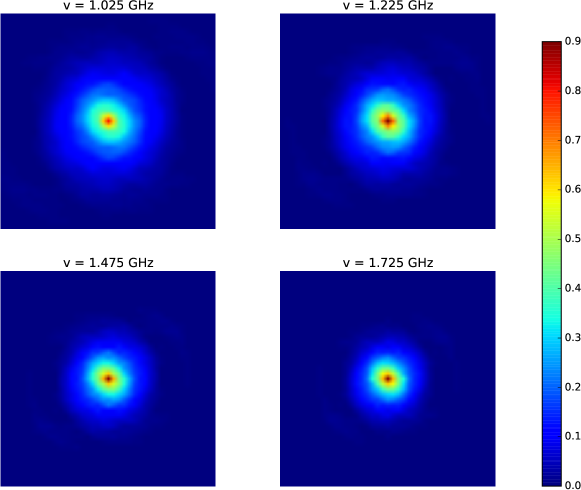
The PSFs used in this simulation where computed using the MeqTrees package (Noordam and Smirnov, 2010) with MeerKAT arrays configuration. We simulated $\ell_{\nu}=15$ frequency bands. The first is centered at 1.025 GHz. The central frequencies of the 15 bands are separated by 50 MHz. The total observation time is 8 hours. The size in pixels of the images are $256\times 256$. Figure 1 shows $50\times 50$ pixels images of the center of the PSF at four frequencies (1.025 HZ, 1.225 GHz, 1.475 GHz and 1.725GHz). The parameters $\mu_{\epsilon}$, $\mu_{s}$ and $\mu_{\nu}$ control the levels of regularization (resp. smoothing, spatial and spectral). They have been set to $\mu_{\epsilon}=0.001$, $\mu_{s}=0.5$ and $\mu_{\nu}=1.0$. The augmented Lagragian parameters $\rho_{P}$, $\rho_{T}$, $\rho_{V}$ and $\rho_{S}$ affect the speed of convergence. They have been set to $\rho_{P}=1.0$, $\rho_{T}=5.0$, $\rho_{V}=2.0$ and $\rho_{S}=1.0$. The classical termination criterion for the ADMM algorithm is that the primal and dual residuals must be small (Boyd et al., 2011). In order to avoid additional parameters, the algorithm will be simply stopped after 350 iterations in the following simulations.

Figure 1. PSFs of MeerKAT in 4 among the 15 simulated frequency bands. The PSFs are obtained from MeqTrees. The total observation time is 8 hours. The images are a $50\times 50$ pixels zoom of the central region.

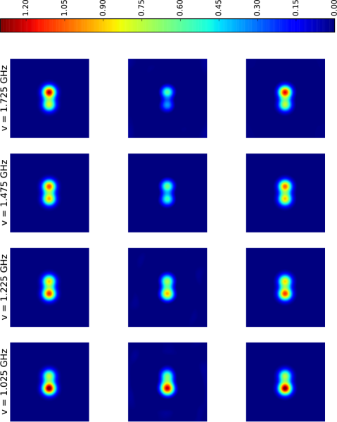
The first simulation evaluates the ability of the algorithm to reconstruct spectra. The sky image is similar to the first simulation of (Rau and Cornwell, 2011). It consists in two overlapping Gaussian profiles centered at pixel 108 and 148, with constant spectral indices equal to respectively -1.0 and +1.0.

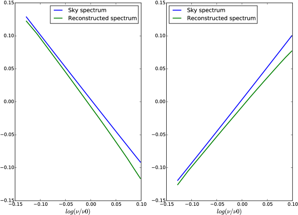
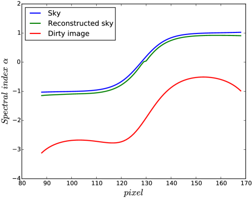
Figure 2 shows in four frequency bands: the sky image, the dirty image and the reconstructed sky obtained using algorithm 1. Figure 3 shows the spectra associated to the pixel at the center of each Gaussian. In each case the theoretical spectrum and the reconstructed spectrum are plotted. In order to derive a synchrotron spectral index map, each spectrum of the original sky (which equals here a linear combination of $\nu$ and $1/\nu$) is fitted to a second order power law model; i.e. $\alpha\log(\nu)+\beta\log^{2}(\nu)$ in a log scale. Spectral indices are then estimated fitting the same model to the reconstructed spectra. Figure 4 shows the estimated $\alpha$ for the pixels on the line joining the center of the two Gaussian profiles. The spectral indices estimated directly from the dirty image are given in the figure for comparison. These preliminary simulations show the ability of the proposed method to reconstruct complex spectral signatures using a non parametric approach.

Figure 2. Multi-frequency reconstruction results. Each line is associated to a frequency band. The first column is the original object. The second column is the dirty image and the third column the reconstructed object. The second column (dirty images) is scaled down in order to fit to the color map of the two other columns.

Figure 3. Spectra associated to the pixel at the center of each Gaussian profile. Sky model in blue and reconstructed sky model in green.

Figure 4. Estimated spectral indices for the pixels on the line joining the center of the two Gaussian profiles. Sky model in blue, reconstructed sky model in green and dirty image in red.

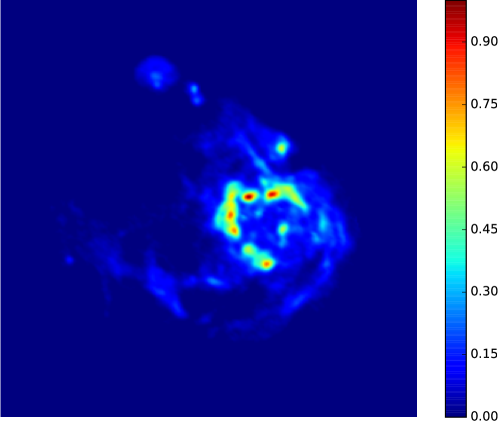
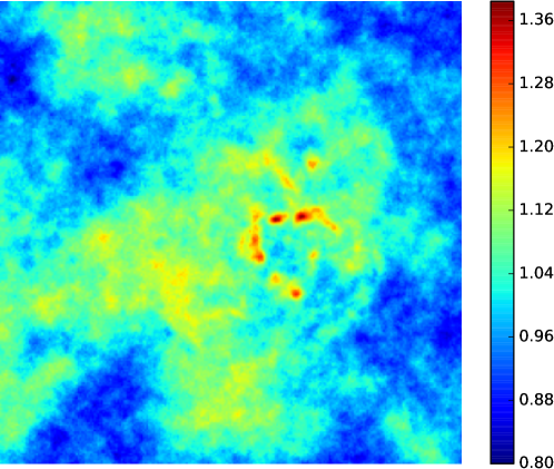
The scope of the second simulation is to evaluate the performances of the method in a more realistic scenario. Radio emission from an HII region in the M31 galaxy is used as a reference sky image. A sky cube is then computed applying a first order power-law spectrum model to the M31 image. The $256\times 256$ map of spectral indices is constructed following the procedure detailed in (Junklewitz et al., 2014): for each pixel the spectral index $\alpha$ is a linear combination of an homogeneous Gaussian field and the reference sky image. The first correlates the spectral indices spatially and the second correlates in a pixel the spectral index with the object intensity. Figure 5 shows the sky map and a typical spectral indices map. A white gaussian noise with a constant variance corresponding to a signal to noise ratio of 20 dB has been added to all the dirty images.

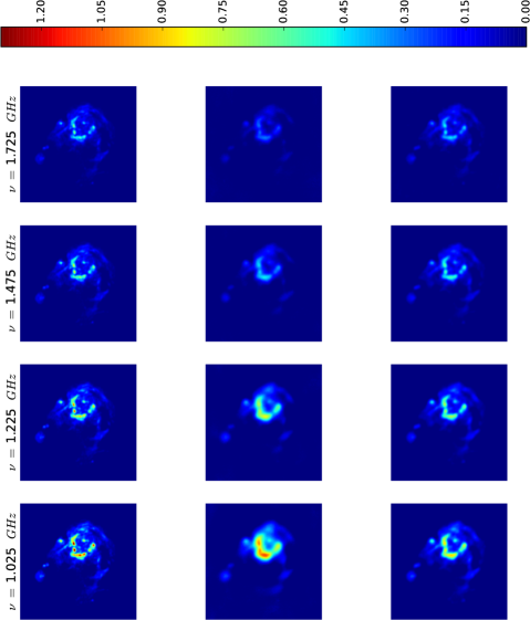
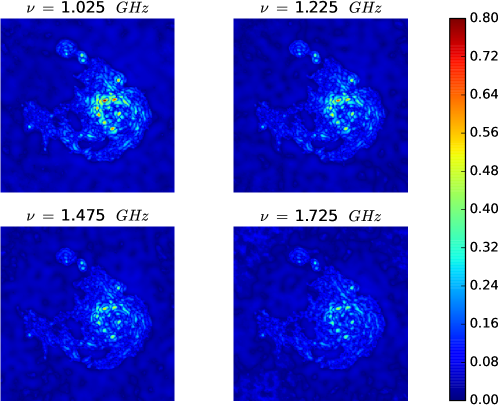
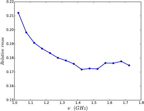
The computation time required to reconstruct the $256\times 256\times 15$ pixels cube, using $\nu_{\ell}=15$ cores is approximately 1.5 hours. Figure 6 shows in four frequency bands: the sky image, the dirty image and the reconstructed map. Figure 7 shows for the same frequency bands the error images between the sky and the reconstructed sky (square root of the absolute value of the difference between the two images). Finally, figure 8 gives the relative root mean square error (RMSE) as a function of the frequency band. These results clearly show the capacity of the algorithm to recover details of the sky image at every frequency.

Figure 5. Radio emission from an HII region in the M31 galaxy and a spectral indices map generated combining the sky intensity and a Gaussian homogeneous random field.

Figure 6. Multi-frequency reconstruction results. Each line is associated to a frequency band. The first column is the original sky. The second column is the dirty image and the third column the reconstructed sky. The second column (dirty images) is scaled down in order to fit to the color map of the two other columns.

Figure 7. Error between the sky and the reconstructed sky. The images show the square root of the absolute value of the difference between the two images.

Figure 8. Relative root mean square error (RMSE) of the reconstructed sky as a function of the frequency.

5. Conclusion

This paper presents first results on multi-frequency image reconstruction for radio interferometry using a fully regularized inverse problem approach. The proposed algorithm relies on the minimisation of a data fidelity term spatially and spectrally regularized. An efficient iterative algorithm is derived to minimize the related convex cost function. The computational bottleneck of the algorithm can be parallelized w.r.t. the images at each frequency leading to an overall computation time of the order of narrow-band algorithms. Future work will focus among others on the derivation of specific spectral regularizations and on the necessity of taking into account frequency-dependent instrumental effects such as a the primary-beam.

References

- Bajkova and Pushkarev (2011) A.T. Bajkova and A.B. Pushkarev. Multifrequency synthesis algorithm based on the generalized maximum entropy method: application to 0954+658. Monthly Notices of the Royal Astronomical Society, 417(1):434–443, October 2011.
- Boyd et al. (2011) S. Boyd, N. Parikh, E. Chu, B. Peleato, and J. Eckstein. Distributed optimization and statistical learning via the alternating direction method of multipliers. Foundations and Trends in Machine Learning, 3(1):1–122, 2011.
- Carrillo et al. (2012) R.E. Carrillo, J.D. McEwen, and Y. Wiaux. Sparsity Averaging Reweighted Analysis (SARA): a novel algorithm for radio-interferometric imaging. Monthly Notices of the Royal Astronomical Society, 426(2):1223–1234, October 2012.
- Carrillo et al. (2014) R.E. Carrillo, J.D. McEwen, and Y. Wiaux. PURIFY: a new approach to radio-interferometric imaging. Monthly Notices of the Royal Astronomical Society, 439(4):3591–3604, April 2014.
- Conway et al. (1990) J. E. Conway, T. J. Cornwell, and P. N. Wilkinson. Multi-frequency synthesis - a new technique in radio interferometric imaging. Monthly Notices of the Royal Astronomical Society, 246(3):490, 1990.
- Dabbech et al. (2015) A. Dabbech, C. Ferrari, D. Mary, E. Slezak, O. Smirnov, and J. S. Kenyon. MORESANE: MOdel REconstruction by Synthesis-ANalysis Estimators. Astronomy and Astrophysics, 576:A7, 2015.
- Dewdney et al. (2013) P.E. Dewdney, W. Turner, R. Millenaar, R. McCool, J. Lazio, and T. J. Cornwell. SKA1 system baseline design. Technical Report SKA-TEL-SKO-DD-001 Revision: 1, SKA Organisation, 2013.
- Eckstein and Bertsekas (1992) J. Eckstein and D. P. Bertsekas. On the Douglas-Rachford splitting method and the proximal point algorithm for maximal monotone operators. Mathematical Programming, 55:293–318, 1992.
- Elad et al. (2007) M. Elad, P. Milanfar, and R. Rubinstein. Analysis versus synthesis in signal priors. Inverse Problems, 23(3):947, 2007.
- Garsden et al. (2015) H. Garsden, J. N. Girard, J.-L. Starck, S. Corbel, C. Tasse, A. Woiselle, J.P. McKean, et al. LOFAR sparse image reconstruction. Astronomy and Astrophysics, 575:A90, March 2015.
- Hestenes and Stiefel (1952) M. R. Hestenes and E. Stiefel. Methods of conjugate gradients for solving linear systems. Journal of research of the National Bureau of Standards, 49:409–436, 1952.
- Högbom (1974) J. A. Högbom. Aperture Synthesis with a Non-Regular Distribution of Interferometer Baselines. AAPS, 15:417–426, June 1974.
- Junklewitz et al. (2014) H. Junklewitz, M.A. Bell, and T. Enßlin. A new approach to multi-frequency synthesis in radio interferometry. arXiv.org, page 4711, January 2014.
- Kellermann (1974) K.I. Kellermann. Galactic and Extragalactic Radio Astronomy, chapter Radio galaxies and quasars. Springer-Verlag, 1974.
- Kraus (1986) J. D. Kraus. Radio Astronomy. Cygnus-Quasar, Powell, Ohio, 1986.
- Noordam and Smirnov (2010) J.E. Noordam and O.M. Smirnov. The MeqTrees software system and its use for third-generation calibration of radio interferometers. Astronomy and Astrophysics, 524:A61, December 2010.
- Rau and Cornwell (2011) U. Rau and T. J. Cornwell. A multi-scale multi-frequency deconvolution algorithm for synthesis imaging in radio interferometry. Astronomy and Astrophysics, 532:71, August 2011.
- Scaife and Heald (2012) A.M.M. Scaife and G.H. Heald. A broad-band flux scale for low-frequency radio telescopes. Monthly Notices of the Royal Astronomical Society: Letters, 423(1):L30–L34, June 2012.
- Schutz et al. (2014) A. Schutz, A. Ferrari, D. Mary, et al. Painter: a spatiospectral image reconstruction algorithm for optical interferometry. JOSAA, 31(11), Nov 2014.
- Thiébaut et al. (2013) É. Thiébaut, F. Soulez, and L. Denis. Exploiting spatial sparsity for multi-wavelength imaging in optical interferometry. JOSAA, 30(2):160–170, February 2013.
- Wenger and Magnor (2014) S. Wenger and M. Magnor. A sparse reconstruction algorithm for multi-frequency radio images. Technical report, Computer Graphics Lab, TU Braunschweig, November 2014.