Effective dynamics of microorganisms that interact with their own trail

Abstract

Like ants, some microorganisms are known to leave trails on surfaces to communicate. We explore how trail-mediated self-interaction could affect the behavior of individual microorganisms when diffusive spreading of the trail is negligible on the timescale of the microorganism using a simple phenomenological model for an actively moving particle and a finite-width trail. The effective dynamics of each microorganism takes on the form of a stochastic integral equation with the trail interaction appearing in the form of short-term memory. For moderate coupling strength below an emergent critical value, the dynamics exhibits effective diffusion in both orientation and position after a phase of superdiffusive reorientation. We report experimental verification of a seemingly counterintuitive perpendicular alignment mechanism that emerges from the model.

For many animals and microorganisms it is advantageous to know where their companions or they themselves have been Couzin (2009); Passino et al. (2008); Reid et al. (2012); Ben-Jacob et al. (2000); Chowdhury et al. (2004); Jackson et al. (2006); Bonner and Savage (1947); Kaiser and Crosby (1983); Wu et al. (2007). To this end, many creatures leave trails of some characteristic substance. A well studied example is the pheromone trails of ants Jackson et al. (2006); Sumpter and Beekman (2003), which allows them to collect food efficiently. Single cell organisms are also known to leave trails Burchard (1982); Zhao et al. (2013). It is believed that the trails help them form aggregates in sparse populations Bonner and Savage (1947); Kaiser (2007); Zhao et al. (2013), whereas in denser populations, colonies could also result from the combined effect of surface-bound motility and excluded volume interactions Peruani et al. (2012); Soto and Golestanian (2014). For bacteria, these trails are often subsumed as exopolysaccharides (EPS) Sutherland (2001) but may also contain proteins Dworkin and Kaiser (1993). To be evolutionarily favorable, the (energetic) costs incurred by trail formation should balance the advantages gained through this form of communication.

Chemotaxis is commonly mediated by rapidly diffusing signalling molecules Bonner and Savage (1947) but, more generally, cell-cell signalling can also be mediated by trails of macromolecules that diffuse much more slowly than the microorganism or form stable gels Sutherland (2001); Christensen and Characklis (1990). Chemically-mediated interactions between bacteria or eukaryotic cells Brenner et al. (1998); Ben-Jacob et al. (2000); Tsori and De Gennes (2004); Taktikos et al. (2011, 2012); Levine and Rappel (2013); Gelimson and Golestanian (2015) as well as artificial active colloids Golestanian (2012); Cohen and Golestanian (2014); Saha et al. (2014) lead to a variety of collective phenomena including collapse, pattern formation, alignment and oscillations. Auto-chemotactic effects have been studied in the context of swimming bacteria Grima (2005); Sengupta et al. (2009) and Dictyostelium cells Westendorf et al. (2013). While much is known about the chemotactic machinery in bacteria Sourjik and Berg (2004); Tu and Grinstein (2005) and eukaryotic cells Levine and Rappel (2013), relatively little is known about trail-mediated interactions.

Whereas ants have antennae that are spatially well separated from their pheromone glands Hangartner (1967), such a clear separation is difficult for single-celled organisms Dworkin and Kaiser (1993); Thar and Kühl (2003); Herzmark et al. (2007). In addition to sensing the trails left by other individuals, microorganisms are also immediately affected by their own trails. This suggests that trail-mediated self-interaction could play a significant role in the behavior of microorganisms. For example, by providing a mechanism to tune the effective translational and orientational diffusivities, or by creating distinct modes of motility, and consequently, the search strategy.

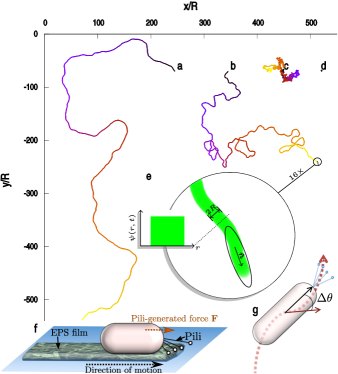
Figure 1: (color online). Sample trajectories generated by the effective dynamics, Eqs. (1a,1c,1d), over a period of time $10^{3}\tau$ (color coded) for: no interaction with the trail, $\Omega\tau\equiv 0$ (a), weak interaction, $\Omega\tau=1.2$ (b), strong interaction, $\Omega\tau=1.85$ (c), close to the localization transition, and above it, $\Omega\tau=2.15$ (d). The rotational diffusivity is set to $D_{r}^{0}\tau=10^{-2}$, and $2\tau$ is the trail crossing time. Panel (e) shows a magnification of the end of trail b with the trail field, $\psi(\bm{r},t)$, of width $2R$ in green and the current orientation of the microorganism (ellipse), $\bm{\hat{n}}$. (f) Schematic depiction of a microscopic model system such as P. aeruginosa that uses pili for motility and sensing. (g) A schematic for the definition of $\Delta\theta$, which is the angle between the current body orientation and the bacterial trajectory (dotted line).

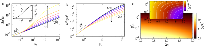
Figure 2: (color online). Angular MSD $\delta\varphi^{2}(t)$ (a), and translational MSD $\delta r^{2}(t)$ normalized by the trail width, $R$, (b) as a function of time $t$ for several values of the effective turning rate $\Omega\tau=0,0.4,0.7,1.0,1.3,1.6,1.9$. The microscopic diffusivity is set to $D_{r}^{0}\tau=0.1$. The inset of (a) shows $`\delta\varphi^{2}(t)$ for $\Omega\tau=1.99$ demonstrating the intermediate superballistic regime. (c) Color coded translational diffusivity $D$ normalized by the trail width $R$ and the trail crossing time $\tau$ as a function of the control parameters. Note the logarithmic axes. Inset: The translational diffusivity for the same range of parameters normalized by the trail free ($\Omega\tau\equiv 0$) value $D^{0}$ on a linear scale. The white contour lines are $0.1$ apart.

In this Letter, we discuss a simple but generic model of a microorganism experiencing trail-mediated interactions. Focusing on a persistent EPS trail with vanishing diffusivity but taking its finite width explicitly into account, we focus on the immediate self-interaction that previously had to be excluded a priori by an ad hoc refractory period ten Hagen et al. (2011); Taktikos et al. (2012). While previous work has mostly considered a concentration dependent speed Tsori and De Gennes (2004); Grima (2005); Sengupta et al. (2009), a coupling to the orientation arises naturally Taktikos et al. (2011); Saha et al. (2014); Note (2). We find that the self-trail interaction modifies the translational and orientational motion of the microorganisms and renormalize the corresponding diffusion coefficients, at the longest time scale (see Fig. 1).

Microscopic Model.—

We consider a single particle of width $2R$ whose state at time $t$ is defined by its position $\bm{r}(t)$ and orientation $\bm{\hat{n}}(t)=(\cos\varphi,\sin\varphi)$. We model the dynamics by prescribing a fixed characteristic speed, $v_{0}$, for the particle, namely

$$\partial_{t}\bm{r}(t)=v_{0}\bm{\hat{n}}(t).$$ (1a)

The motion will typically be generated via the cooperation of a number of molecular motors, whether it is realized by the retraction of pili Skerker and Berg (2001); Holz et al. (2010), the extrusion of slime Wolgemuth et al. (2002), or any other mechanism. This implies significant noise in the propulsion force, and consequentially, a finite directional persistence. For the simplest, trail-free case, we model the orientational dynamics as a purely diffusive process, $$\partial_{t}\varphi(t)=\xi(t) \xi(t) \left\langle\xi(t)\xi(t^{\prime})\right\rangle=2D_{r}^{0}\delta(t-t^{\prime}) D_{r}^{0} 1/D_{r}^{0} \delta r^{2}(t)=\left\langle[\bm{r}(t)-\bm{r}(0)]^{2}\right\rangle \delta r^{2}(t)=v_{0}^{2}t^{2} D_{r}^{0}t\ll 1 \delta r^{2}(t)=4D^{0}t D_{r}^{0}t\gg 1 D^{0}=v_{0}^{2}/(2D_{r}^{0}) v_{0}$$, where is a Gaussian random variable obeying and is the microscopic rotational diffusion coefficient controlling the persistence time . This trail-free model displays a translational mean-square displacement (MSD) that crosses over from ballistic, , for, , to diffusive behavior, , for where . Fluctuations in could also be taken into account in a straightforward generalization Peruani and Morelli (2007).

The trail excreted from the microorganism can be characterized by the density profile $\psi(\bm{r},t)$ that satisfies the diffusion equation $\partial_{t}\psi(\bm{r},t)-{\cal D}_{\rm p}\nabla^{2}\psi(\bm{r},t)=k\delta_{R}^{2}\left(\bm{r}-\bm{r}(t)\right)$, where $k$ is the deposition rate and $\delta_{R}^{2}\left(\bm{r}-\bm{r}(t)\right)$ is a “regularized delta function” that accounts for the finite size $R$, and traces its position [normalized as $\int d^{2}r\,\delta_{R}^{2}(\bm{r})=1$]. Setting ${\cal D}_{\rm p}=0$, we find for the trail profile at time $t$ and position $\bm{x}$ as

$$\psi(\bm{x},t)=k\int_{0}^{t}dt^{\prime}\,\delta_{R}^{2}\left(\bm{x}-\bm{r}(t^{\prime})\right).$$ (1b)

We choose a rectangular source, $\delta_{R}^{2}(\bm{r})=\Theta(R^{2}-r^{2})/\pi R^{2}$, where $\Theta(x)$ denotes the Heaviside step function and $r\equiv|\bm{r}|$. The trail width $2R$ defines a microscopic time scale $\tau=R/v_{0}$, which gives the trail crossing time (see Fig. 1e). This specific regularization scheme is a good representation of the regime in which the characteristic diffusion length of the polymeric trail is much smaller than the width of the trail, $\sqrt{{\cal D}_{\rm p}\tau}\ll R$ Note (1).

A generic interaction with the trail couples to gradients of the trail field perpendicular to the current orientation Taktikos et al. (2012); Saha et al. (2014), effectively steering the microorganism toward trails by favouring a orientation $\bm{\hat{n}}$ perpendicular to the trail, i.e.,

$$\partial_{t}\varphi(t)=\chi\partial_{\perp}\psi(\bm{r}(t),t)+\xi(t),$$ (1c)

where $\partial_{\perp}\psi=\bm{\hat{n}}_{\perp}(t)\cdot\nabla\psi(\bm{r}(t),t)$, with $\bm{\hat{n}}_{\perp}=(-\sin\varphi,\cos\varphi)$ being the angular unit vector in polar coordinates. The sensitivity to the trail is controlled by a parameter $\chi$. We have provided a microscopic derivation of this coupling Note (2) for a model system of a pili-driven bacterium on a substrate (see Fig. 1f) by assuming a generic dependence of the pili surface attachment force on the EPS concentration. However, Eq. (1c) will be expected in the continuum limit for any microscopic model based on symmetry considerations Saha et al. (2014).

Effective Dynamics.—

We assume that the particle trajectory does not bend back on itself immediately (no-small-loops assumption), and that self-intersections on longer times are rare enough to be negligible.

By making a short time expansion of Eqs. (1a) and (1c) to be inserted into Eq. (1b), one finds a closed equation for the head of the trail field $\partial_{\perp}\psi(t)\equiv\partial_{\perp}\psi(\bm{r}(t),t)$ Note (2). The result is a stochastic integral equation

$$\partial_{\perp}\psi(t)=\frac{\Omega}{\tau}\int_{0}^{\tau}du\,(\tau-u)\,[\partial_{\perp}\psi(t-u)+\xi(t-u)/\chi],$$ (1d)

The effective turning rate $\Omega=k\chi\tau/\pi R^{3}$ increases for more intense trails (larger $k$) and for more sensitive organisms (larger $\chi$). The delay $\tau$ reflects the memory imparted by the trail. The closed set of equations (1a,1c,1d) constitute our effective dynamical description of the system.

For the average gradient one finds $\left\langle\partial_{\perp}\psi\right\rangle\sim\exp(\alpha t)$ where the rate $\alpha$ is given implicitly as the solution of $\lambda(\alpha)=0$ where $\lambda(\alpha)=1-\frac{\Omega\tau}{\alpha\tau}\left[1+\frac{1}{\alpha\tau}\left(e^{-\alpha\tau}-1\right)\right]$. For $\Omega\tau<2$, $\alpha<0$ and Eq. (1d) defines a random process with zero mean that leads to a stationary dynamics which is time-translation invariant. For $\Omega\tau>2$ one finds $\alpha>0$, i.e., the gradient (angular velocity) diverges exponentially in time. Implying that the trajectory converges in a logarithmic spiral to a localized point. This means there is a maximum value of the product of trail deposition rate and sensitivity, $k\chi$, that allows steady-state motion. For sample trajectories, see Figs. 1 and 3.

In the stationary regime, Eq. (1d) can be solved in the frequency domain, $\chi\widetilde{\partial_{\perp}\psi}(\omega)=[\lambda^{-1}(i\omega)-1]\tilde{\xi}(\omega)$. The trail-mediated self-interaction thus linearly transforms the intrinsic white noise $\xi$ to an effective colored random angular velocity, $\tilde{\Xi}(\omega)=\tilde{\xi}(\omega)/\lambda(i\omega)$ such that $\partial_{t}\varphi(t)=\Xi(t)$.

Angular & Translational MSD.—

The most easily accessible quantity in experiments is the translational MSD $\delta r^{2}(t)$, which is related to the angular MSD, $\delta\varphi^{2}(t)=\left\langle[\varphi(t)-\varphi(0)]^{2}\right\rangle$, via Doi and Edwards (1988)

$$\delta r^{2}(t)=2v_{0}^{2}\int_{0}^{t}dt^{\prime}\,(t-t^{\prime})\,e^{-\delta\varphi^{2}(t^{\prime})/2}.$$ (2)

The angular MSD is a sum of three terms, given in the Laplace domain as $s^{2}\widehat{\delta\varphi^{2}}(s)/(2D_{r}^{0})=1+\widehat{\Delta}(s)+\widehat{\Lambda}(s).$ The corrections to simple diffusion are given by the two correlation functions $\Lambda(t):=\chi\left\langle\partial_{\perp}\psi(t)\xi(0)\right\rangle/(2D_{r}^{0})$ (such that $\hat{\Lambda}(s)=\lambda^{-1}(s)-1$) and $\Delta(t)=\chi^{2}\left\langle\partial_{\perp}\psi(t)\partial_{\perp}\psi(0)\right\rangle/D_{r}^{0}=2\int_{0}^{t}dt^{\prime}\Lambda(t^{\prime})\Lambda(t^{\prime}+t)$. The definition of $\hat{\Lambda}(s)$ shows that $\Omega\tau$ is the only relevant control parameter for the orientational MSD $\delta\varphi^{2}(t)$ and the behavior of $\delta\varphi^{2}(t)$ is fully determined by the analytic structure of $\lambda^{-1}(s)$.

In the stationary regime, $\delta\varphi^{2}(t)$ (cf. Fig. 2a Note (3)) starts off diffusively, $\delta\varphi^{2}(t)=2D_{r}^{0}t$ for $t\ll\tau$ and becomes asymptotically diffusive again, $\delta\varphi^{2}(t)=2D_{r}t$ for $t\gg\tau/(1-\Omega\tau/2)$ determined by the smallest pole of $\lambda^{-1}(i\omega)$. The effective orientational diffusivity

$$D_{r}/D_{r}^{0}=1+\frac{\Omega\tau}{2}\times\frac{1+\Omega\tau/2}{(1-\Omega\tau/2)^{2}},$$ (3)

diverges for $\Omega\tau\to 2$ confirming our expectation that the trail-mediated self-interaction reduces orientational persistence. The two diffusive regimes are joined by an intermediate, superdiffusive regime. Note that the crossover time to the asymptotic diffusive regime diverges as $\Omega\tau\to 2$. Close to the limiting value $\Omega\tau=2$, the crossover is given by the super-ballistic law $\delta\varphi^{2}(t)=6D_{r}^{0}\tau(t/\tau)^{3}$ for $\tau\ll t\ll\tau/(1-\Omega\tau/2)$. For a fast effective turning rate $\Omega>D_{r}^{0}$, the intrinsic noise combines a diffusive ($\propto t^{1/2}$) excursion with the ballistic ($\propto t$) reorientation due to the self-interaction, leading to $\delta\varphi(t)\propto t^{3/2}$ until later times where the stochastic character of the self-interaction becomes important and turns the behavior back to diffusion.

The translational MSD $\delta r^{2}(t)$ always starts ballistically, $\delta r^{2}(t)=v_{0}^{2}t^{2}$ for $t\ll\tau$ and crosses over to diffusive behavior $\delta r^{2}(t)=4Dt$ for long times $t\to\infty$ (cf. Fig. 2b). The crossover time, $t^{*}$ will be determined implicitly by $\delta\varphi^{2}(t^{*})\sim 1$. For the location of the crossover and the dependence of the translational diffusivity on the control parameters, we have to consider a number of different regimes.

Short Persistence Regime.—

When $(D_{r}^{0}\tau)^{-1}<1+\Omega\tau/2$, the crossover happens around $\Omega t\sim\sqrt{1+2\Omega/D_{r}^{0}}-1$ and the asymptotic diffusivity

$$D/D^{0}=\sqrt{\pi D_{r}^{0}/2\Omega}\,e^{D_{r}^{0}/2\Omega}\operatorname{erfc}(\sqrt{D_{r}^{0}/2\Omega}),$$ (4)

is a function of the ratio $D_{r}^{0}/\Omega$ alone.

Long Persistence Regime.—

For sufficiently straight trails such that by the time $\delta\varphi^{2}(t)\sim 1$ it is already deep in the long time diffusive regime, i.e., $D_{r}^{0}\tau\ll 2(1-\Omega\tau/2)^{3}/[2-\Omega\tau+(\Omega\tau)^{2}/2]$, the crossover happens around $t\sim 1/D_{r}$ and the asymptotic diffusivity is given as

$$D/D^{0}=\frac{D_{r}^{0}}{D_{r}}\left[1-\frac{(D_{r}^{0}\tau)^{2}}{6}\frac{\Omega\tau(1+\Omega\tau/2)^{3}}{(1-\Omega\tau/2)^{6}}\right].$$ (5)

Critical Regime.—

Close to the upper limit $\Omega\tau\to 2$ and for $D_{r}^{0}\tau<1$, the crossover happens around $t/\tau\sim 1/\sqrt[3]{D_{r}^{0}\tau}$ and the asymptotic diffusivity

$$D/D^{0}=\Gamma(3/4)(D_{r}^{0}\tau)^{2/3}+D_{r}^{0}\tau/3,$$ (6)

is a function of $D_{r}^{0}\tau$ alone. Note that the dependence on the intrinsic noise, $D\propto 1/\sqrt[3]{D_{r}^{0}}$, is significantly weakened compared to the trail free case, $D^{0}\propto 1/D_{r}^{0}$, and that $D$ does not vanish as $\Omega\tau\to 2$.

Intermediate Regime.—

In the rest of the parameter space of $D_{r}^{0}\tau$ and $\Omega\tau$, no explicit expressions can be given and the asymptotic diffusivity $D$ will be a function of both control parameters. Numerical result for the effective translational diffusivity is presented in Fig. 2c.

Discussion.—

The interaction of a microorganism with its own trail effectively introduces a new timescale $1/\Omega$. The trail-mediated self-interaction modulates the intrinsic noise in a linear but nontrivial way. While the asymptotic dynamics remains diffusive below the critical value $\Omega\tau=2$, both for the translational and the orientational degrees of freedom, the (orientational) diffusive regime may only be reached on timescales that may be much longer than $\tau$. This holds in the limit of strong interactions where the crossover timescale $\tau/(1-\Omega\tau/2)$ becomes increasingly large but also for large effective persistence times $1/D_{r}$. Moreover, the crossover times are distinct from the microscopic persistence time $1/D_{r}^{0}$.

The asymptotic angular diffusivity, $D_{r}$, is a function of $\Omega\tau$ that diverges as $\Omega\tau\to 2$. It is always larger than its microscopic value $D_{r}^{0}$, i.e., orientational persistence is reduced by the trail. The translational diffusivity, $D$, on the other hand, is always reduced and, in general, depends on the parameters $\Omega\tau$ and $D_{r}^{0}\tau$.

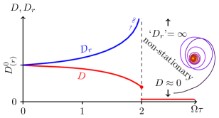
Figure 3: (color online). Phase diagram of the dynamics of the microorganism with trail-mediated self-interaction, as a function of the dimensionless turning frequency $\Omega\tau$. Inset: Zoomed view of Fig. 1d.

For very strong trail-mediated self-interactions, $\Omega\tau>2$, the initial dynamics quickly confines the particle in a region of size $\lesssim 2R$. Here, our assumptions break down and the ensuing dynamics will depend on more microscopic details not resolved in the present model. Nevertheless, we can formally identify the behavior of the microorganism by a diverging rotational diffusivity. The translational diffusivity incurs a finite jump at the transition point as it is determined by the regular short-time part of $\delta\varphi^{2}(t)$ below the transition and by unresolved microscopic details above it. We note that the no-small-loops condition, which can be written as $\delta\varphi^{2}(\tau)\sim(\Omega\tau)^{2}(D_{r}^{0}\tau)^{2}<\pi^{2}$, does not obscure this phase transition, so long as $D_{r}^{0}\tau<1$. The analysis of a more microscopic model is beyond the scope of this contribution. The behavior of the system can be summarized in a phase diagram as shown in Fig. 3. Our findings are subtly different from the sub-diffusion observed in Ref. Chepizhko and Peruani (2013) as a result of temporary trapping of bacteria in loops caused by quenched disorder, which is a stationary regime.

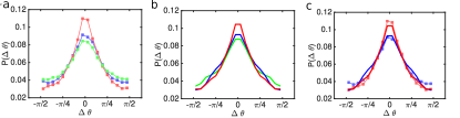
Figure 4: (color online). (a) The experimentally observed narrowing of the $\Delta\theta$ distribution with increasing trail deposition (see Fig. 1g for the definition of $\Delta\theta$). The experiments were carried out with the P. aeruginosa mutants $\Delta psl$, which does not secrete Psl (light green) and $\Delta$P_psl/P_BAD-psl, which secretes Psl in response to the arabinose in the environment. For $\Delta$P_psl/P_BAD-psl, the arabinose concentration was varied between $0\%$ (light blue, low Psl deposition) and $1\%$ (light red, high Psl deposition). (b) The corresponding theoretical $\Delta\theta$ distributions resulting from the influence of the alignment term. The trail coupling strength is varied between $\Omega\tau=0.05$ (green) $\Omega\tau=0.12$ (blue) and $\Omega\tau=0.35$ (red). The distribution has been sampled using the time interval of $\Delta t=0.2\,\tau$, and the rotational diffusion has been set to $D_{r}^{0}\tau=0.015$. These values roughly correspond to the experimental parameters at which the distribution has been measured. (c) A comparison between experimental (dots) and theoretical (lines) distributions of $\Delta\theta$ for the $\Delta$P_psl/P_BAD-psl mutant under $0\%$ (blue) and $1\%$ arabinose (red).

The perpendicular alignment strategy might appear to be counter-intuitive, but it is supported by recent experimental evidence. We have investigated this question by probing the angle distributions of single bacteria in experimentally recorded motion of P. aeruginosa with different rates of Psl exopolysaccharide deposition (in a similar experiment to Ref. Zhao et al. (2013)); for methods, see the Supplemental Material Note (2). For the angle $\Delta\theta$ between the trajectory and the body orientation (defined in Fig. 1g), the experiments show that the distribution narrows down with increasing increasing the secretion of Psl trails in via a mutant with an arabinose inducible promoter, which increases the effective trail deposition strength; see Figs. 4b and c. Our numerical simulations of the model predict a similar trend, as shown in Fig. 4b and c, highlighting the interplay between the noise and the tendency of perpendicular alignment. The trail can have a stabilizing effect by reorienting the microorganism towards the inner regions in case it reaches the trail boundaries. The result is a significantly narrower $\Delta\theta$ distribution with increasing $\Omega$, indicating a higher correlation between trajectory and microorganism orientation. Further evidence in support of the perpendicular alignment scenario can be extracted from the collective behavior of the bacteria New-Gelimson-etal .

Our results could have significant biological (as well as biophysical Note (2)) implications. Regulating the strength of the trail-mediated self-interaction may allow microorganisms to decide whether to confine themselves to smaller areas and search them more thoroughly or explore larger areas. Interestingly, the effective translational diffusion coefficient scales as $1/\sqrt[3]{D_{r}^{0}}$ in the presence of strong trail-mediated self-interaction, as compared to $1/D_{r}^{0}$ in the trail-free case. This suggests that trails make the microorganism less sensitive to intrinsic variations in the orientational noise.

To conclude, we have shown that a very simple model of particle-trail interaction leads to a wealth of nontrivial phenomena, including an transition from stationary to non-stationary behavior with a diverging orientational diffusivity. Our results could shed light on the behavior of trail-forming microorganisms, and in particular how they can use this “expensive” output to regulate their own activity while, simultaneously, providing a communication channel with other individuals. Moreover, they could also find use in the field of robotics by providing a blue-print for designing micro-robots that can tune their search strategy via local interactions with their own trails.

Appendix A Microscopic derivation of the equations of motion

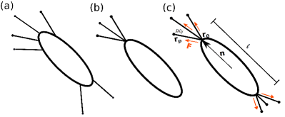
Figure 5: Schematics of pili distribution around a bacterium. (a) Asymmetric distribution around the body (N. gonorrhoae). (b) Pili concentrated at one pole (P. aeruginosa). (c) Idealized model with a symmetric distribution of pili at the poles.

We regard a bacterium of length $\ell$ which secretes an EPS film and pulls itself forward using typically $N$ pili, Fig. 5. We will assume that the pili attach to the surface in an EPS-dependent way. Better attachment results in more effective pulling and therefore we can assume that the pulling force of an individual pilus attached at site $\bm{r}_{i}$ is EPS-dependent, $f=f(\psi(\bm{r}_{i}))$. The distribution of pili on the surface of bacteria varies among species. They may be scattered all over the surface (Fig. 1a), or concentrated in one (Fig. 1b), or both poles (Fig. 1c) Maier (2013). The general argument given below holds for all these pilus configurations but to be concrete, we will assume a symmetric distribution of an equal number of pili, concentrated at the two poles. The attachment sites are assumed to be distributed randomly according to some distribution $P(\bm{r}_{i}-\bm{r}_{0};\bm{\hat{n}})=P(\bm{r}_{p};\bm{\hat{n}})=P(r_{p},\vartheta)$, where $\bm{r}_{0}$ is the head (or tail) of a bacterium, $\bm{r}_{p}$ is the relative coordinate of the pilus tip, and $\vartheta$ is the angle between $\bm{\hat{n}}$ and $\bm{r}_{p}$. We assume that the force $\bm{f}_{i}=f(\psi(\bm{r}_{i}))\bm{\hat{e}}_{p}$ will pull along the direction of $\bm{r}_{p}$. It is plausible to assume that the probability for directions in which pili can face is symmetrically distributed around the body orientation $\bm{\hat{n}}$. This implies that $\int\bm{\hat{e}}_{p}P(\bm{r}_{p};\bm{\hat{n}})d^{2}r_{p}\parallel\bm{\hat{n}}$. If this was not the case, the pili would preferentially explore the space right/left of the body and there would be, to a first approximation, a constant torque turning the microorganism in one direction.

We assume that $\psi(\bm{r})$ is a smooth function on the scale of a typical pilus length $\langle r_{p}\rangle$ and can be expanded as

$$f(\psi(\bm{r}_{i}))=f(\psi(\bm{r}_{0}))+f^{\prime}(\psi(\bm{r}_{0}))[\nabla\psi(\bm{r}_{0})\cdot\bm{r}_{p}]+\mathcal{O}(\bm{r}_{p}^{2})$$

where $f^{\prime}\equiv\partial_{\psi}f(\psi)$.

We can then use this to approximate the average total force $\langle\bm{F}\rangle=\langle\sum_{i}\bm{f}_{i}\rangle$

$$\langle\bm{F}\rangle\approx N\int d^{2}r_{p}P(\bm{r}_{p};\bm{\hat{n}})f(\psi(\bm{r}_{0}+\bm{r}_{p}))\bm{\hat{e}}_{p}$$

$$\approx F(\psi(\bm{r}_{0}))\bm{\hat{n}}\int_{-\pi}^{\pi}\!\!\cos\vartheta P(\vartheta)d\vartheta$$

$$+F^{\prime}(\psi(\bm{r}_{0}))\nabla\psi(\bm{r}_{0})\cdot\int d^{2}r_{p}P(\bm{r}_{p};\bm{\hat{n}})r_{p}\bm{\hat{e}}_{p}\bm{\hat{e}}_{p}$$

The pili force component parallel to the bacterial body will leave the orientation of the bacterium unchanged and propel the centre of mass of the bacterium. The average propelling force will be

$$\langle\bm{F}_{\parallel}\rangle=\bm{\hat{n}}(\bm{\hat{n}}\cdot\langle\bm{F}\rangle)\approx\bm{\hat{n}}F(\psi(\bm{r}_{0}))\langle\cos\vartheta\rangle$$ (7)

In an overdamped system, the velocity of the microorganism will be proportional to the pulling force $\partial_{t}\bm{r}=\mu_{\parallel}\langle\bm{F}_{\parallel}\rangle=v_{0}\bm{\hat{n}}$ where $\mu_{\parallel}$ is the translational mobility. This gives equation (1a) with

$$v_{0}(\psi)=\mu_{\parallel}F(\psi(\bm{r}))\langle\cos\vartheta\rangle$$ (8)

The velocity of the microorganism is in general $\psi$-dependent but in case of a large constant contribution of $\bm{F}$, the $\psi$-dependent contribution to the velocity will be subdominant.

The perpendicular component of the pulling force $\bm{F}_{\perp}=\bm{F}-\bm{\hat{n}}(\bm{\hat{n}}\cdot\bm{F})$, on the other hand, will generate a torque on the body of the microorganism and here, the EPS dependence of the force needs to be taken into account even at the lowest order. The average torque is given by $\langle\bm{\tau}\rangle=(\ell/2)\bm{\hat{n}}\times\langle\bm{F}\rangle$. Using Eq. (A) we get

$$\langle\bm{\tau}\rangle\approx\frac{\ell}{2}F^{\prime}(\psi(\bm{r}_{0}))[\bm{\hat{n}}\times\nabla\psi(\bm{r}_{0})]\langle r_{p}\sin^{2}\vartheta\rangle$$ (9)

and a completely equivalent equation for the torque coming from pili pulling at the other tip of the microorganism.

On a surface the motion of the microorganism will be overdamped and therefore the angular velocity $\mathbf{\omega}$ will be linear to the sum of the torques from both tips

$$\frac{d\bm{\hat{n}}}{dt}=-\bm{\hat{n}}\times\mathbf{\omega} \approx-\mu_{\perp}\bm{\hat{n}}\times\langle\bm{\tau}_{\text{head}}+\bm{\tau}_{\text{tail}}\rangle$$ (10)

$$=-\chi\bm{\hat{n}}\times(\bm{\hat{n}}\times\nabla\psi)$$

where $\mu_{\perp}$ is the rotational mobility and

$$\chi(\psi)=\mu_{\perp}\ell F^{\prime}(\psi(\bm{r}))\langle r_{p}\sin^{2}\vartheta\rangle$$ (11)

which becomes independent of $\psi$ if $F^{\prime}(\psi)\approx$ const.

In addition to this deterministic reorientation, we should also account for noise due to thermodynamic fluctuations and fluctuations in pili attachment, which result in torque fluctuations. For the case that the pili pulling direction is correlated only on a very short time scale (i.e. the pili attach according to $P(\bm{r}_{p})$ much quicker than the microorganism moves), we obtain the stochastic equation

$$\frac{d\bm{\hat{n}}}{dt}=-\chi\bm{\hat{n}}\times(\bm{\hat{n}}\times\nabla\psi)+\bm{\hat{n}}\times\mathbf{\xi}_{r}$$ (12)

This equation can be rewritten in terms of the orientation angle $\varphi$ relative to some axis on the surface by defining $\bm{\hat{n}}=(\cos\varphi,\sin\varphi)^{T}$, which gives Eq. (1c).

Appendix B Derivation of Equation (1d)

From the definition of the trail field we have

$$\nabla_{\bm{x}}\psi(\bm{x},t)=-\frac{2k}{\pi R^{2}}\int_{0}^{t}dt^{\prime}[\bm{x}-\bm{r}(t^{\prime})]\delta(R^{2}-|\bm{x}-\bm{r}(t^{\prime})|^{2})$$

and with a change of variables $t^{\prime}\to t-t^{\prime}$,

$$\partial_{\perp}\psi(\bm{r}(t),t)=-\frac{2k}{\pi R^{2}}\int_{0}^{t}dt^{\prime}[\bm{r}(t)-\bm{r}(t-t^{\prime})]\cdot\bm{\hat{n}}_{\perp}(t)\\ \times\delta(R^{2}-|\bm{r}(t)-\bm{r}(t-t^{\prime})|^{2})$$ (13)

From the twice iterated integral

$$\bm{r}(t-\tau)=\bm{r}(t)+v_{0}\int_{t}^{t-\tau}du\bm{\hat{n}}(t)+v_{0}\int_{t}^{t-\tau}du\int_{0}^{u}dw\dot{\bm{\hat{n}}}(w)$$

one finds $[\bm{r}(t)-\bm{r}(t-\tau)]^{2}=v_{0}^{2}\tau^{2}+\mathcal{O}(\tau^{3})$ and

$$[\bm{r}(t)-\bm{r}(t-\tau)]\cdot\bm{\hat{n}}_{\perp}(t)=-v_{0}\int_{0}^{\tau}du\int_{0}^{u}dw\{\chi\bm{\hat{e}}_{z}\cdot[\bm{\hat{n}}(t-w)\times\nabla\psi(\bm{r}(t-w),t-w)]+\xi(t-w)\}\bm{\hat{n}}_{\perp}(t-w)\cdot\bm{\hat{n}}_{\perp}(t)$$

An identical iteration shows $\bm{\hat{n}}_{\perp}(t-w)\cdot\bm{\hat{n}}_{\perp}(t)=1+\mathcal{O}(w)$ and thus

$$[\bm{r}(t)-\bm{r}(t-\tau)]\cdot\bm{\hat{n}}_{\perp}(t)\\ =-v_{0}\int_{0}^{\tau}du\int_{0}^{u}dw[\chi\partial_{\perp}\psi(t-w)+\xi(t-w)]+\mathcal{O}(\tau^{3})$$ (14)

Using the above two approximations in Eq. (13) and performing one of the integrals yields Eq. (1d).

Appendix C Implications on experimental measurements of diffusivities

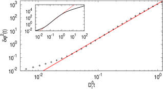
Figure 6: Angular MSD $\delta\varphi^{2}(t)$ as a function of time $t$ for $\Omega\tau=1.94$, $D_{r}^{0}\tau=0.1$ (black crosses) and a power law fit (red line) $\propto t^{2.64}$ for $D_{r}^{0}t\in[0.05,1]$. The inset shows the same plot over a larger time window, showing that the fit does not capture the asymptotic behavior.

The MSD curve in Fig. 6 highlights subtleties that must be considered when interpreting such measurements in terms of a model, and for extracting model parameters. The long time diffusivity, $D_{r}$, is not the bare diffusivity $D_{r}^{0}$ as determined by the cellular motility apparatus. Moreover, the asymptotic diffusive regime is reached on very long time scales only: timescales on the order of hours , and that may well be beyond experimental reach, and even beyond the life time of microorganisms. In that case, it might be tempting to conclude that the MSDs show anomalous diffusion asymptotically; as can be seen from Fig. 6, an anomalous exponent $\beta\approx 2.64$ can fit the data extremely well.

Appendix D Experimental Methods and Sample Preparation

P. aeruginosa PAO1 holloway1955genetic strains $\Delta psl$ – a strain that does not produce Psl – as well as $\Delta$P_psl/P_BAD-psl ma2006analysis – an engineered Psl-inducible strain – were used in this study. For the detailed experimental information such as culture conditions, flow cell assembly and image capture system, please refer to methods in Zhao et al. (2013). An overnight bacteria culture in FAB medium heydorn2000experimental supplemented with 30mM glutamate, was diluted and injected into a flow cell. FAB medium with 0.6 mM glutamate was continuously pumped through the flow chamber using a syringe pump with a flow rate of 3ml/hour at 30^∘C. Different amounts of arabinose were added into the medium to control the production of Psl. Bright-field images were taken every 3 seconds by an EMCCD camera on an Olympus IX81 microscope equipped with Zero Drift autofocus system. The image size is $67\times 67\mu{\rm m}^{2}$ ($1024\times 1024\text{ pixel}^{2}$). A typical data set has about 14000$-$20000 frames and contains up to 1,000,000 bacteria images.