$2$-branes with Arnold-Beltrami Fluxes
from Minimal $D=7$ Supergravity
P. Fré${}^{\;a1,a2,c}$ and A.S. Sorin${}^{\;b,c}$
^a1Dipartimento di Fisica, Universitá di Torino
^a2INFN – Sezione di Torino
via P. Giuria 1,  10125 Torino  Italy
e-mail:  fre@to.infn.it
^bBogoliubov Laboratory of Theoretical Physics and
Veksler and Baldin Laboratory of High Energy Physics
Joint Institute for Nuclear Research,
141980 Dubna, Moscow Region, Russia

e-mail: sorin@theor.jinr.ru
^cNational Research Nuclear University MEPhI
(Moscow Engineering Physics Institute),
Kashirskoe shosse 31, 115409 Moscow, Russia

We describe this paper as a Sentimental Journey from Hydrodynamics to Supergravity. Beltrami equation in three dimensions that plays a key role in the hydrodynamics of incompressible fluids has an unsuspected relation with minimal supergravity in seven dimensions. We show that just $D=7$ supergravity and no other theory with the same field content but different coefficients in the lagrangian, admits exact two-brane solutions where Arnold-Beltrami fluxes in the transverse directions have been switched on. The rich variety of discrete groups that classify the solutions of Beltrami equation, namely the eigenfunctions of the $\star d$ operator on a three-torus, are by this newly discovered token injected into the brane world. A new quite extensive playing ground opens up for supergravity and for its dual gauge theories in three dimensions, where all classical fields and all quantum composite operators will be assigned to irreducible representations of discrete crystallographic groups $\Gamma$.

1 Introduction

The canvas of this paper can be provocatively described as a Sentimental Journey from Hydrodynamics to Supergravity. The main character of this play is a simple first order differential equation written in the XIX century by the great Italian Mathematician Eugenio Beltrami[1]: an equation that bears his name and can be cast in the following modern notation:

$$\star\,\mathrm{d}\mathbf{Y}_{[1]}\,=\,\mu\,\mathbf{Y}_{[1]}$$ (1.1)

That above is an eigenvalue problem for a $1$-form $\mathbf{Y}_{[1]}$ and makes sense only on three-manifolds $\mathcal{M}_{3}$. If $\mathcal{M}_{3}$ is compact, the spectrum of the $\star\,\mathrm{d}$ operator is discrete and encodes topological properties of the manifold. In particular if $\mathcal{M}_{3}$ is a flat torus $T^{3}$, all the spectrum of eigenvalues and eigenfunctions can be constructed with simple algorithms and it can be organized into irreducible representations of a rich variety of crystallographic groups that were recently explored and classified by the two of us [2]. The hydrodynamical viewpoint on eq.(1.1) arises from the trivial observation that a $1$-form $\mathbf{Y}_{[1]}$ is dual to a vector field ${\mathbf{V}}$ and that any vector field in three-dimensions can be interpreted as the velocity field of some fluid. This hydrodynamical interpretation of eq.(1.1) is boosted by the existence of a very important theorem proved by V. Arnold [3]: on compact manifolds $\mathcal{M}_{3}$, streamlines of a steady flow have a chance of displaying a chaotic behavior only if the one-form dual to the vector-field of the flow satisfies Beltrami equation.

Yet one-forms can also be interpreted as gauge fields and one can conceive the idea of using the solutions of eq.(1.1) in their primary capacity, namely as ingredients in classical solutions of some gauge-theory. Due to the strictly euclidian signature of the metric utilized in eq.(1.1) one is naturally led to imagine that the manifold $\mathcal{M}_{3}$ is either part of the internal compact variety in a spontaneous compatification of a higher dimensional theory, typically supergravity, or part of the transverse manifold in a brane-solution of the same. Ah! Here we are: flux-branes! This is the word! Arnold-Beltrami fields can change their profession and from flows they can be turned into fluxes. Once the first seed of this change of perspective is planted the tree grows fast and the idea develops along logical lines. If our target are $p$-branes, then we need to decide how large is $p$ and our final goal will be the world-volume gauge–theory $\mathcal{GT}_{p+1}$ in $p+1$-dimensions. The lowest reasonable choice is $p=2$, leading to three-dimensional world-volume gauge-theories that can be Maxwell Chern Simons. The challenging perspective is the following. If we are able to find exact supergravity solutions of the $2$-brane type that have Arnold-Beltrami fluxes in the transverse directions, then the discrete crystallographic symmetry group $\Gamma$ of the fluxes will be transmitted to the $2$-brane classical supergravity solution and from the latter to the $\mathcal{GT}_{3}$ on the world volume. This scenario is quite attractive since it envisages, for the first time, a systematic and rich injection of discrete group symmetries into the brane–world: the journey from hydrodynamics to supergravity starts being quite interesting if not sentimental! In order to proceed we have to count dimensions carefully. Three dimensions are occupied by the world volume, another three by a $T^{3}$ torus transverse to the brane. This makes already six. Hence we have to look at six-dimensional supergravity or higher. A guiding line comes from another constraint. If we want a two-brane, in the bosonic spectrum of the considered supergravity there should be a gauge three-form $\mathbf{B}^{[3]}$ that will couple to the world-volume of the brane. Then six-dimensional supergravity is not sufficient since it contains only gauge two-forms $\mathbf{B}^{[2]}$ (for $D=6$ supergravities see [4],[5],[6],[7],[8]). The first favorable case is $D=7$: here we have minimal supergravity, that contains 16 supercharges and it is usually named $\mathcal{N}=2$ since the 16 supercharges are arranged into a pair of pseudo-Majorana spinors. Supergravities in seven dimensions were constructed (up to four fermion terms) in the mid eighties in several papers [9],[10], [11],[12],[13],[14]. The Poincaré (ungauged) version of the minimal theory was independently constructed by Townsend and van Nieuwenhuizen [9] and by Salam and Sezgin [10] in two different formulations that use respectively a three-form gauge field $\mathbf{B}^{[3]}_{\mu\nu\rho}$ and a two-form gauge field $\mathbf{B}^{[2]}_{\mu\nu}$, in addition to the graviton $g_{\mu\nu}$, the gravitino $\Psi_{A|\mu}^{\alpha}$ ($\alpha=1,\dots,8$, $\mu\,=\,0,1,\dots,6$, $A\,=\,1,2$), the gravitello $\chi_{A}^{\alpha}$, three gauge fields $\mathcal{A}^{\Lambda}_{\mu}$ ($\Lambda\,=\,1,2,3$) and the dilaton $\phi$, that are common to both formulations. From the on-shell point of view the number of degrees of freedom described by either $\mathbf{B}^{[3]}_{\mu\nu\rho}$ or $\mathbf{B}^{[2]}_{\mu\nu}$ is the same and the two types of gauge fields are electric-magnetic dual to each other.

This field content constitutes excellent news for our $2$-brane plans. Either in an electric or in a magnetic formulation we have at our disposal a $\mathbf{B}^{[3]}$ form which can couple to the $2$-brane world volume. In addition the triplet of gauge fields $\mathcal{A}^{\Lambda}$ is a very encouraging starting point for Arnold-Beltrami fluxes. Indeed the theory has a global symmetry $\mathrm{SO(3)}$ under which the three vector fields $\mathcal{A}^{\Lambda}$ transform in the defining representation (which in this case coincides with the adjoint): hence they are specially prepared to be identified with triplets of Arnold-Beltrami one-forms transforming in any three dimensional representation of any discrete subgroup $\Gamma\subset\mathrm{SO(3)}$. If such fluxes can be consistently switched on within the setup of a $2$-brane solution, such solution will be invariant under $\Gamma$ and this symmetry will descend to the gauge theory on the world volume.

There is only one question that remains open: what about the $7$th dimension? At first sight it seems a sort of uninvited guest that hangs around without purpose, yet we know that in supergravity and supersymmetry nothing is ever superfluous, nothing sits there without a deep reason: on the contrary, like in a well built swiss watch, all the wheels, larger or smaller are equally essential to the proper working of the whole thing. A suggestion comes from our previous experience with fractional $D3$-branes [15], [16],[17].

Considering in particular the smooth realization [15] of the fractional D3-brane as a $3$-brane solution of $D=10$ type IIB supergravity in which the transverse space to the brane world–volume is of the form:

$$\mbox{transverse space to the D3-brane}\,=\,\mbox{ALE}_{4}\,\times\,\mathbb{R}^{2}$$ (1.2)

we see something similar to what we are faced with in $D=7$. The fractional D3-brane is a flux-brane where the doublet of gauge two-forms $\mathbf{B}^{\Lambda}_{[2]}$ develop geometrical fluxes, being identified with linear combinations of the non trivial cohomology two-cycles $\omega^{I}_{[2]}$ that leave on the four-dimensional $\mathrm{ALE}$-space: $\mathbf{B}^{\Lambda}_{[2]}\,=\,\gamma^{\Lambda}_{I}\,\omega^{I}_{[2]}$. At first sight also in this case the extra flat dimensions associated with $\mathbb{R}^{2}$ seem unnecessary spectators. Actually this is not true. The coefficients $\gamma^{\Lambda}_{I}$ introduced one line above have to be functions of the extra coordinates $x,y$ on $\mathbb{R}^{2}$ and using the natural complex structure $z\,=\,x+{\rm i}y$ they happen to be holomorphic functions $\gamma^{\Lambda}_{I}\,=\,\gamma^{\Lambda}_{I}(z)$ of the coordinate $z$. These holomorphic functions play an essential role in establishing the overall supergravity solution.

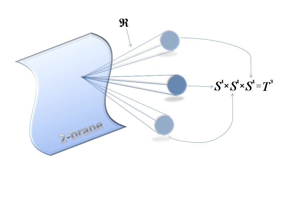
Figure 1: A metaphoric view of the two-brane structure in $D=7$. The transverse space to the two-brane world-volume is the direct product of a three torus $T^{3}$, homeomorphic to three circles $\mathbb{S}^{1}\times\mathbb{S}^{1}\times\mathbb{S}^{1}$ with a straight line $\mathbb{R}$. The Arnold Beltrami fluxes live on $\mathrm{T}^{3}$ but are embedded into supergravity with coefficients that have a predetermined exponential dependence from the coordinate $U$ of $\mathbb{R}$. In some sense $U$ measures the distance from the $2$-brane that is a boundary for $D=7$ space-time.

Hence, mutatis mutandis, we are lead to consider a similar situation where the transverse space to our candidate $2$-brane is the following one:

$$\mbox{transverse space to the 2-brane}\,=\,T^{3}\,\times\,\mathbb{R}$$ (1.3)

The torus $T^{3}$ is the compact manifold which replaces the $\mathrm{ALE}$-space and the Arnold-Beltrami one-forms $\mathbf{Y}^{I}_{[1]}$, leaving on the torus, play the role played by the cohomology two-cycles leaving on $\mathrm{ALE}$. The triplet of gauge fields $\mathcal{A}^{\Lambda}$ play in $D=7$ the same role that was played in $D=10$ by the doublet of two forms $\mathbf{B}^{\Lambda}_{[2]}$, namely they develop fluxes being identified with linear combinations of the Arnold-Beltrami one-forms:

$$\mathcal{A}^{\Lambda}\,=\,\gamma^{\Lambda}_{I}\,\mathbf{Y}^{I}_{[1]}$$ (1.4)

The catch is that the coefficients $\gamma^{\Lambda}_{I}$ have to be functions of the unique coordinate $U$ on $\mathbb{R}$:

$$\gamma^{\Lambda}_{I}\,=\,\gamma^{\Lambda}_{I}(U)$$ (1.5)

It remains to be understood which functional condition on the $\gamma^{\Lambda}_{I}(U)$ replaces the holomorphicity pertaining to the D3-brane case. We will see that the $\gamma^{\Lambda}_{I}(U)$ are constrained to have an exponential dependence:

$$\gamma^{\Lambda}_{I}(U)\,=\,e^{\mu\,U}\,\mathcal{E}^{\Lambda}_{\phantom{\Lambda}I}$$ (1.6)

where $\mu$ is the eigenvalue of $\star\,\mathrm{d}$-operator in Beltrami equation (1.1) and $\mathcal{E}^{\Lambda}_{\phantom{\Lambda}I}$ denotes a constant embedding matrix whose group-theoretical structure we discuss in later sections. The overall conception of the proposed $2$-branes with Arnold-Beltrami fluxes is graphically and metaphorically summarized in fig.1.

All what we have discussed so far materializes into a definite ansatz for all the bosonic fields of minimal $D=7$ supergravity and the question is whether such an ansatz does or does not satisfy the field equations of supergravity. In full analogy with the case of the D3-brane we expect that all the field equations should reduce, upon use of the advocated ansatz, to a unique differential equation of the following form:

$$\Box_{T^{3}\times\mathbb{R}}\,H(U,\mathbf{X})\,=\,\mathbf{j}(U,\mathbf{X})$$ (1.7)

where $H(U,\mathrm{X})$ is a scalar function of the transverse coordinates that enters the $D=7$ brane-like metric:

$$ds^{2}\,=\,H(U,\mathbf{X})^{-\frac{8}{5\,\Delta}}\,d\xi^{\mu}\otimes d\xi^{\nu}\,\eta_{\mu\nu}\,-\,H(U,\mathbf{X})^{\frac{12}{5\,\Delta}}\,\left(dU^{2}\,+\,dX^{2}\,+\,dY^{2}\,+\,dZ^{2}\right)$$ (1.8)

The source function $\mathbf{j}(U,\mathbf{X})$ appearing in eq.(1.7) should be uniquely defined, as in the D3-brane case by the fluxes and should vanish at zero fluxes. In that case $H(U,\mathbf{X})$ is a harmonic function.

In the present paper we show that the above expectations are indeed fulfilled and that $2$-branes with Arnold-Beltrami fluxes are exact solutions of minimal $D=7$ supergravity. Actually we show something even stronger. While $2$-brane-solutions without fluxes do exist for any bosonic theory that has the same field content as minimal supergravity but not necessarily the specific coefficients imposed by supersymmetry, Arnold-Beltrami flux $2$-branes are a specific feature of supergravity. All the field equations reduce to equation (1.7) if and only if the lagrangian coefficients are in the precise ratios predicted by the supergravity construction of [9],[11]. This implies, in particular, that $\Delta\,=\,4$ in eq. (1.8).

Hence quite unexpectedly Beltrami equation (1.1) has a hidden and deep relation with supersymmetry that is unveiled by the existence of the flux-branes presented in this paper. The injection of discrete symmetries into the brane–world turns out to be a successful operation and the Sentimental Journey from Hydrodynamics to Supergravity has a happy starting. However, we must stress that Rev. Yorick has just disembarked in Calais and that he has only exchanged snuff boxes with his monk acquaintance: the road to Paris and to the South is still long. We need to derive equations for the Killing spinors and to determine the supersymmetries preserved by the flux-branes, we need to discuss their fate in the gauged version of the theory and their analogue in curved backgrounds. All that requires a firm control on the lagrangian, the transformation rules and the gaugings.

The gauging of $D=7$ minimal supergravity was also independently considered both in [9] and in [10]. The coupling of minimal $D=7$ supergravity to $n$ vector multiplets was constructed by Bergshoeff et al in [11] on the basis of the two-form formulation and shown to be founded on the use of the coset manifold:

$$\mathcal{M}_{3n+1}\,=\,\mathrm{SO(1,1)}\,\times\,\frac{\mathrm{SO(3,n)}}{\mathrm{SO(3)\times SO(n)}}$$ (1.9)

as scalar manifold that encodes the spin zero degrees of freedom of the theory.

In all the quoted references the construction was done using the Noether coupling procedure, up to four-fermion terms in the Lagrangian and up to two-fermion and three-fermion terms in the transformation rules. Correspondingly the on-shell closure of the supersymmetry algebra was also checked only up to such terms. Furthermore the possible addition of new topological interaction terms was proposed but never proved.

In consideration of the renewed interest in this particular supergravity theory in relation with the Arnold-Beltrami flux-branes, a separate collaboration involving one of us [24] is presently reconsidering the reconstruction of minimal $D=7$ supergravity and its gauging in the approach based on Free Differential Algebras and rheonomy (for reviews see [25] and also the second volume of [26]). The goal is that of clarifying the algebraic structure underlying the theory and perfectioning its construction to all fermion orders. The issue, as we will demonstrate, is particularly relevant in connection with gauging since there the FDA structure becomes essential and comes into contact with the formalism of the embedding tensor [30, 31].

We postpone the discussion of Killing spinors and of the preserved supersymmetries to the moment when the results of [24] will be available.

1.1 Organization of the paper

Since some of the concepts, of the definitions and of the mathematical techniques heavily used in [2] are not common in Particle Physics and Supergravity, we devote section 2 to a comprehensive summary of these topics, introducing here and there in our presentation a change of perspective which takes into account the different goals pursued by this paper. Particulary important for the understanding of what will follow is sect. 2.5 and its subsection 2.5.4. In the latter we recall the notion of the Universal Classifying Group which has been invented by the two us in [2] and plays a key role both in the Hydrodynamical and in the Supergravity interpretation of Beltrami equation.

Sect.3 summarizes the classification of Arnold-Beltrami one-forms obtained in [2] showing its bearing on the issue of flux-branes.

Sect. 4 contains a detailed discussion of the space group $\mathrm{GF_{192}}\subset\mathrm{G_{1536}}$ which is the $\Gamma$-symmetry group of the explicit examples of Arnold-Beltrami flux branes presented in this paper. Let us also stress that this section contains the precise discussion of how the discrete symmetry groups of Beltrami flows are transmitted to supergravity.

Sect.s 4.1,4.2,4.3,4.4 present the explicit construction of the triplets of Arnold-Beltrami one-forms utilized in the afore mentioned examples. The transformation of these triplets under $\mathrm{GF_{192}}$ or one of its subgroups are carefully discussed here.

Sect. 5 and 6 contain the core result of this paper announced in the introduction, namely the derivation of the $2$-brane solutions of minimal $D=7$ supergravity having Arnold Beltrami fluxes in the transverse space.

Sect. 7 contains our conclusions.

In the appendices we provide tables of the conjugacy classes of the group $\mathrm{GF_{192}}$ and of its subgroup $\mathrm{GS_{24}}$.

A part of the material presented in this paper repeats that presented in [2]. We did these repetitions to make the present paper self-consistent both conceptually and technically. Furthermore we have discarded all those items of [2] that are not pertinent to our present goals and that might even be source of confusion in the present interpretation of Arnold-Beltrami one forms.

2 Crystallographic Lattices, the Torus $T^{3}$ and Discrete Groups

As we explained in the introduction, we are interested in $2$-brane solutions of a gravitational gauge theory, identifiable with minimal $D=7$ Supergravity, where the vector fields develop fluxes that are Beltrami fields on a three torus transverse to brane world-volume:in this way the discrete symmetry groups of such fluxes will be transmitted to the brane solution and to the brane gauge- theory. In the present section, in order to fix notations and to clarify our working setup, we summarize some essential facts about crystallographic lattices and about the algorithmic construction of Beltrami fields on the three-tours; in this we closely follow our previous paper [2].

Topologically the three torus is defined as the product of three circles, namely:

$$\mathrm{T}^{3}\,\equiv\,\mathbb{S}^{1}\,\times\,\mathbb{S}^{1}\,\times\,\mathbb{S}^{1}\,\equiv\,\frac{\mathbb{R}}{\mathbb{Z}}\,\times\,\frac{\mathbb{R}}{\mathbb{Z}}\,\times\,\frac{\mathbb{R}}{\mathbb{Z}}$$ (2.1)

Alternatively we can define the three-torus by modding $\mathbb{R}^{3}$ with respect to a three dimensional lattice. In this case the three-torus comes automatically equipped with a flat constant metric:

$$\mathrm{T}^{3}_{g}\,=\,\frac{\mathbb{R}^{3}}{\Lambda}$$ (2.2)

According to (2.2) the flat Riemaniann space $\mathrm{T}^{3}_{g}$ is defined as the set of equivalence classes with respect to the following equivalence relation:

$${\mathbf{r}}^{\prime}\,\sim\,{\mathbf{r}}\quad\mbox{iff}\quad{\mathbf{r}}^{\prime}\,-\,{\mathbf{r}}\,\in\,\Lambda$$ (2.3)

The metric (2.5) defined on $\mathbb{R}^{3}$ is inherited by the quotient space and therefore it endows the topological torus (2.1) with a flat Riemaniann structure. Seen from another point of view the space of flat metrics on $\mathrm{T}^{3}$ is just the coset manifold $\mathrm{SL(3,\mathbb{R})}/\mathrm{O(3)}$ encoding all possible symmetric matrices, alternatively all possible space lattices, each lattice being spanned by an arbitrary triplet of basis vectors (2.4). So let us consider the standard $\mathbb{R}^{3}$ manifold and introduce a basis of three linearly independent 3-vectors that are not necessarily orthogonal to each other and of equal length:

$${\mathbf{w}}_{\mu}\,\in\,\mathbb{R}^{3}\quad\mu\,=\,1,\dots\,3$$ (2.4)

Any vector in $\mathbb{R}$ can be decomposed along such a basis and we have: ${\mathbf{r}}\,=\,r^{\mu}{\mathbf{w}}_{\mu}$. The flat (constant) metric on $\mathbb{R}^{3}$ is defined by:

$$g_{\mu\nu}\,=\,\langle{\mathbf{w}}_{\mu}\,,\,{\mathbf{w}}_{\nu}\rangle$$ (2.5)

where $\langle\,,\,\rangle$ denotes the standard euclidian scalar product. The space lattice $\Lambda$ consistent with the metric (2.5) is the free abelian group (with respect to sum) generated by the three basis vectors (2.4), namely:

$$\mathbb{R}^{3}\,\ni\,{\mathbf{q}}\,\in\,\Lambda\,\Leftrightarrow\,{\mathbf{q}}\,=\,q^{\mu}\,{\mathbf{w}}_{\mu}\quad\mbox{where}\quad q^{\mu}\,\in\,\mathbb{Z}$$ (2.6)

The momentum lattice is the dual lattice $\Lambda^{\star}$ defined by the property:

$$\mathbb{R}^{3}\,\ni\,{\mathbf{p}}\,\in\,\Lambda^{\star}\,\Leftrightarrow\,\langle{\mathbf{p}}\,,\,{\mathbf{q}}\rangle\,\in\,\mathbb{Z}\quad\forall\,{\mathbf{q}}\,\in\,\Lambda$$ (2.7)

A basis for the dual lattice is provided by a set of three dual vectors ${\mathbf{e}}^{\mu}$ defined by the relations:

$$\langle{\mathbf{w}}_{\mu}\,,\,{\mathbf{e}}^{\nu}\rangle\,=\,\delta^{\nu}_{\mu}$$ (2.8)

so that

$$\forall\,{\mathbf{p}}\,\in\,\Lambda^{\star}\quad{\mathbf{p}}\,=\,p_{\mu}\,{\mathbf{e}}^{\mu}\quad\mbox{where }\quad p_{\mu}\,\in\,\mathbb{Z}$$ (2.9)

Every lattice $\Lambda$ yields a metric $g$ and every metric $g$ singles out an isomorphic copy $\mathrm{SO_{g}(3)}$ of the continuous rotation group $\mathrm{SO(3)}$, which leaves it invariant:

$$M\,\in\,\mathrm{SO_{g}(3)}\quad\Leftrightarrow\quad M^{T}\,g\,M\,=\,g$$ (2.10)

By definition $\mathrm{SO_{g}(3)}$ is the conjugate of the standard $\mathrm{SO(3)}$ in $\mathrm{GL(3,\mathbb{R})}$:

$$\mathrm{SO_{g}(3)}\,=\,\mathcal{S}\,\mathrm{SO(3)}\,\mathcal{S}^{-1}$$ (2.11)

with respect to the matrix $\mathcal{S}\,\in\,\mathrm{GL(3,\mathbb{R})}$ which reduces the metric $g$ to the Kronecker delta:

$$\mathcal{S}^{T}\,g\,\mathcal{S}\,=\,\mathbf{1}$$ (2.12)

Notwithstanding this a generic lattice $\Lambda$ is not invariant with respect to any proper subgroup of the rotation group $\mathrm{G}\,\subset\,\mathrm{SO_{g}(3)}\,\equiv\,\mathrm{SO(3)}$. Indeed by invariance of the lattice one understands the following condition:

$$\forall\,\gamma\,\in\,\mathrm{G}\quad\mbox{and}\quad\forall\,{\mathbf{q}}\,\in\,\Lambda\,\,:\quad\quad\gamma\,\cdot\,{\mathbf{q}}\,\in\,\Lambda$$ (2.13)

Lattices that have a non trivial symmetry group $\mathrm{G}\subset\mathrm{SO(3)}$ are those relevant to Solid State Physics and Crystallography. There are 14 of them grouped in 7 classes that were already classified in the XIX century by Bravais. The symmetry group $\mathrm{G}$ of each of these Bravais lattices $\Lambda_{B}$ is necessarily one of the well known finite subgroups of the three-dimensional rotation group $\mathrm{O(3)}$. In the language universally adopted by Chemistry and Crystallography for each Bravais lattice $\Lambda_{B}$ the corresponding invariance group $\mathrm{G_{B}}$ is named the Point Group. For purposes different from our present one, the point group can be taken as the lattice invariance subgroup within $\mathrm{O(3)}$ that, besides rotations, contains also improper rotations and reflections. Since we are interested in Beltrami equation, which is covariant only under proper rotations, of interest to us are only those point groups that are subgroups of $\mathrm{SO(3)}$.

According to a standard nomenclature the $7$ classes of Bravais lattices are respectively named Triclinic, Monoclinic, Orthorombic, Tetragonal, Rhombohedral, Hexagonal and Cubic. Such classes are specified by giving the lengths of the basis vectors ${\mathbf{w}}_{\mu}$ and the three angles between them, in other words, by specifying the 6 components of the metric (2.5).

2.1 The proper Point Groups

Restricting one’s attention to proper rotations, the proper point groups that appear in the $7$ lattice classes are either the cyclic groups $\mathbb{Z}_{h}$ with $h=2,3,4$ or the dihedral groups $D_{h}$ with $h=3,4,6$ or the tetrahedral group $\mathrm{T}$ or the octahedral group $\mathrm{O_{24}}$. Here we restrict our attention to lattice with the largest possible Point Group, namely to Cubic Lattice with $\mathrm{O_{24}}$ symmetry (see fig.2).

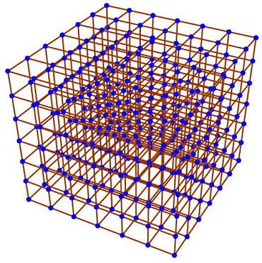
Figure 2: A view of the self-dual cubic lattice

2.2 Group Characters

A fundamental ingredient for our present goals and for those that were pursued in [2] are the characters of the point group and of other classifying groups that have emerged in the constructions we performed in [2].

Given a finite group $\mathrm{G}$, according to standard theory and notations [18] one defines its order and the order of its conjugacy classes as follows:

$$g = \left|\mathrm{G}\right|\,=\,\mbox{$\#$ of group elements}$$

$$g_{i} = \left|\mathcal{C}_{i}\right|\,=\,\mbox{$\#$ of group elements in the conjugacy class $\mathcal{C}_{i}$}\quad i\,=\,i,\dots,r$$ (2.14)

If there are $r$ conjugacy classes one knows from first principles that there are exactly $r$ inequivalent irreducible representation $D^{\mu}$ of dimensions $n_{\mu}\,=\,\mbox{dim}\,D^{\mu}$, such that:

$$\sum_{\mu\,=\,1}^{r}\,n_{\mu}^{2}\,=\,g$$ (2.15)

For any reducible or irreducible representation of dimension $d$:

$$\forall\,\gamma\,\in\,\mathrm{G}\quad:\gamma\,\rightarrow\,\quad\mathfrak{R}\left[\gamma\right]\,\in\,\mbox{Hom}\left[\mathbb{R}^{d}\,,\,\mathbb{R}^{d}\right]$$ (2.16)

the character vector is defined as:

$$\chi^{\mathfrak{R}}\,=\,\left\{\mbox{Tr}\,\left(\mathfrak{R}\left[\gamma_{1}\right]\right)\,,\,\mbox{Tr}\,\left(\mathfrak{R}\left[\gamma_{2}\right]\right)\,,\,\dots,\,\mbox{Tr}\,\left(\mathfrak{R}\left[\gamma_{r}\right]\right)\right\}\,,\quad\gamma_{i}\,\in\,\mathcal{C}_{i}$$ (2.17)

The choice of a representative $\gamma_{i}$ within each conjugacy class $\mathcal{C}_{i}$ is irrelevant since all representatives have the same trace. In particular one can calculate the characters of the irreducible representations:

$$\chi^{\mu}\,=\,\chi\left[D^{\mu}\right]\,\,=\,\left\{\mbox{Tr}\,\left(D^{\mu}\left[\gamma_{1}\right]\right)\,,\,\mbox{Tr}\,\left(D^{\mu}\left[\gamma_{2}\right]\right)\,,\,\dots\,,\,\mbox{Tr}\,\left(D^{\mu}\left[\gamma_{r}\right]\right)\right\}\,,\quad\gamma_{i}\,\in\,\mathcal{C}_{i}$$ (2.18)

that are named fundamental characters and constitute the character table. We stick to the widely adopted convention that the first conjugacy class is that of the identity element $\mathcal{C}_{1}\,=\,\left\{\mathbf{e}\right\}$, containing only one member. In this way the first entry of the character vector is always the dimension $d$ of the considered representation. In the same way we order the irreducible representation starting always with the identity one dimensional representation which associates to each group element simply the number $1$. It is well known that for any finite group $\mathrm{G}$, the character vectors satisfy the following two fundamental relations:

$$\sum_{\mu\,=\,1}^{r}\,\chi_{i}^{\mu}\,\chi_{j}^{\mu}\,=\,\frac{g}{g_{i}}\,\delta_{ij}\quad;\quad\sum_{i\,=\,1}^{r}\,g_{i}\,\chi_{i}^{\mu}\,\chi_{i}^{\nu}\,=\,g\,\delta^{\mu\nu}$$ (2.19)

Utilizing these identities one can immediately retrieve the decomposition of any given reducible representation $\mathcal{R}$ into its irreducible components. Suppose that the considered representation is the following direct sum of irreducible ones:

$$\mathfrak{R}\,=\,\oplus_{\mu=1}^{r}\,a_{\mu}\,D^{\mu}$$ (2.20)

Where $a_{\mu}$ denotes the number of times the irrep $D^{\mu}$ is contained in the direct sum and it is named the multiplicity. Given the character vector of any considered representation $\mathfrak{R}$ the vector of its multiplicities is immediately obtained by use of (2.19):

$$a_{\mu}\,=\,\frac{1}{g}\,\sum_{i}^{r}\,g_{i}\chi_{i}^{\mathfrak{R}}\,\chi_{i}^{\mu}$$ (2.21)

Furthermore one can construct the projectors onto the invariant subspaces $a_{\mu}\,D^{\mu}$ by means of another classical formula that we will extensively use in the sequel:

$$\Pi^{\mu}_{\mathfrak{R}}\,=\,\frac{g_{i}}{g}\,\sum_{k=1}^{r}\,\chi^{\mu}_{k}\,\sum_{\ell\,=\,1}^{g_{k}}\,\underbrace{\mathfrak{R}\left[{\gamma_{\ell}}\right]}_{\gamma_{\ell}\in\,\mathcal{C}_{k}}$$ (2.22)

2.3 The spectrum of the $\star\mathbf{d}$ operator on $\mathrm{T}^{3}$ and Beltrami equation

As we explained in the introduction, the main ingredient of the present paper are the Beltrami one-forms defined over the three-torus $\mathrm{T}^{3}$. By definition these are eigenstates of the $\star_{g}\mathrm{d}$ operator, namely of solutions of the following equation:

$$\star_{g}\mathrm{d}\mathbf{Y}^{(n;I)} = \,\mu_{(n)}\,\mathbf{Y}^{(n;I)}$$ (2.23)

where $\mathrm{d}$ is the exterior differential, and $\star_{g}$ is the Hodge-duality operator which, differently from the exterior differential, can be defined only with reference to a given metric $g$. By $\mathbf{Y}^{(n;I)}$ we denote a one-form:

$$\mathbf{Y}^{(n;I)}\,=\,{\mathbf{Y}}^{(n;I)}_{i}\,dX^{i}\quad;\quad(i\,=\,1,2,3)$$ (2.24)

where the composite index $(n;I)$ makes reference to the quantized eigenvalues $\mu_{(n)}$ of the $\star_{g}\mathrm{d}$ operator (ordered in increasing magnitude $|\mu_{(n)}|$) and to a basis of the corresponding eigenspaces

$$\star_{g}\mathrm{d}\mathbf{Y}^{(n)}\,=\,\,\mu_{(n)}\,\mathbf{Y}^{(n)}\quad\Rightarrow\quad\mathbf{Y}^{(n)}\,=\,\sum_{I=1}^{d_{n}}\,c_{I}\,\mathbf{Y}^{(n;I)}$$ (2.25)

the symbol $d_{n}$ denoting the degeneracy of $|\mu_{(n)}|$ and $c_{I}$ being constant coefficients. Indeed, since $T^{3}$ is a compact manifold, the eigenvalues $\mu_{(n)}$ form a discrete set. We recall the general procedure introduced in [2] to construct the eigenfunctions of $\star_{g}\mathrm{d}$ and to determine their degeneracies. In tensor notation, equation (2.23) has the following appearance:

$$\frac{1}{2}\,g_{ij}\,\epsilon^{jk\ell}\partial_{k}\mathbf{Y}_{\ell}\,=\,m\,\mathbf{Y}_{i}$$ (2.26)

The equation written above is named Beltrami equation since it was already considered by the great italian mathematician Eugenio Beltrami in 1881 [1], who presented one of its periodic solutions previously constructed by Gromeka in 1881[19]. In the case of the cubic lattice, which is our main goal in this paper, the metric is simply given by the Kronecker delta and it can be deleted from the equation, upper and lower indices coinciding. In this way we can rewrite eq.(2.23) in the equivalent way:

$$\frac{1}{2}\,\epsilon_{ijk}\partial_{j}\mathbf{Y}_{k}\,=\,\mu\,\mathbf{Y}_{i}$$ (2.27)

The next task is that of constructing an ansatz for the vector harmonics $\mathbf{Y}_{i}({\mathbf{X}})$ that are eigenfunctions of $\star_{g}\mathrm{d}$. Since such eigenfunctions have to be well defined on $\mathrm{T}^{3}$, their general form is necessarily the following one:

$$\mathbf{Y}_{i}\left({\mathbf{k}}\,|\,{\mathbf{X}}\right) = v_{i}\left({\mathbf{k}}\right)\,\cos\left(2\,\pi\,{\mathbf{k}}\cdot{\mathbf{X}}\right)\,+\,\omega_{i}\left({\mathbf{k}}\right)\,\sin\left(2\,\pi\,{\mathbf{k}}\cdot{\mathbf{X}}\right)$$

$${\mathbf{k}} \in \Lambda^{\star}$$ (2.28)

The condition that the momentum ${\mathbf{k}}$ lies in the dual lattice guarantees that $\mathbf{Y}_{i}({\mathbf{X}})$ is periodic with respect to the space lattice $\Lambda$: $\forall\,{\mathbf{q}}\,\in\,\Lambda\,:\quad Y_{i}\left({\mathbf{X}}\,+\,{\mathbf{q}}\right)\,=\,Y_{i}\left({\mathbf{X}}\right)$. Considering next eq. (2.27) we immediately see that it implies the further condition $\partial^{i}\,Y_{i}\,=\,0$. Imposing such a condition on the general ansatz (2.3) we obtain: ${\mathbf{k}}\,\cdot\,{\mathbf{v}}\left({\mathbf{k}}\right)\,=\,0\quad;\quad{\mathbf{k}}\,\cdot\,{\mathbf{\omega}}\left({\mathbf{k}}\right)\,=\,0$ which reduces the 6 parameters contained in the general ansatz (2.3) to 4. Imposing next the very equation (2.27) we get the following two conditions:

$$\mu\,v_{i}\left({\mathbf{k}}\right) = \pi\,\epsilon_{ij\ell}\,k_{j}\,\omega_{\ell}\left({\mathbf{k}}\right)\quad;\quad\mu\,\omega_{i}\left({\mathbf{k}}\right)\,=\,-\pi\,\epsilon_{ij\ell}\,k_{j}\,v_{\ell}\left({\mathbf{k}}\right)$$ (2.29)

The two equations are self consistent if and only if the following condition is verified: $\mu^{2}\,=\,\pi^{2}\,\langle{\mathbf{k}}\,,\,{\mathbf{k}}\rangle$. This trivial elementary calculation completely determines the spectrum of the operator $\star_{g}\,\mathrm{d}$ on $\mathrm{T}_{g}^{3}$ endowed with the metric fixed by the choice of a lattice $\Lambda$. The possible eigenvalues are provided by:

$$m_{\mathbf{k}}\,=\,\pm\,\pi\,\mbox{det}(w)\,\sqrt{\langle{\mathbf{k}}\,,\,{\mathbf{k}}\rangle}\quad\quad{\mathbf{k}}\,\in\,\Lambda^{\star}$$ (2.30)

The degeneracy of each eigenvalue is geometrically provided by counting the number of intersection points of the dual lattice $\Lambda^{\star}$ with a sphere whose center is in the origin and whose radius is:

$$r\,=\,\sqrt{\langle{\mathbf{k}}\,,\,{\mathbf{k}}\rangle}$$ (2.31)

For a generic lattice the number of solutions of equation (2.31) namely the number of intersection points of the lattice with the sphere is just two: $\pm{\mathbf{k}}$, so that the typical degeneracy of each eigenvalue is just $2$. If the lattice $\Lambda$ is one of the Bravais lattices admitting a non trivial point group $\mathrm{G}$, then the number of solutions of eq.(2.31) increases since all lattice vectors ${\mathbf{k}}$ that sit in one orbit of $\mathrm{G}$ have the same norm and therefore are located on the same spherical surface. The degeneracy of the $\star_{g}\,\mathrm{d}$ eigenvalue is precisely the order of the corresponding $\mathrm{G}$-orbit in the dual lattice $\Lambda^{\star}$.

2.4 The algorithm to construct Arnold Beltrami one-forms

What we explained in the previous section provides a well defined algorithm to construct a series of Arnold Beltrami one-forms quite suitable for a systematic computer aided implementation.

The steps of the algorithm adapted to the case of the cubic lattice $\Lambda\,=\Lambda_{cubic}$ are the following ones:

a)

Consider the character table and the irreducible representations of the Point Group $\mathfrak{P}_{\Lambda}\,=\,\mathrm{O}\,\simeq\,\mathrm{S}_{4}$.

b)

Analyze the structure of orbits of $\mathfrak{P}_{\Lambda}$ on the lattice and determine the number of lattice points contained in each spherical layer $\mathfrak{S}_{n}$ of the dual lattice $\Lambda^{\star}\,=\,\Lambda$ of quantized radius $r_{n}$:

$${\mathbf{k}}_{(n)}\,\in\,\mathfrak{S}_{n}\quad\Leftrightarrow\quad\langle{\mathbf{k}}_{(n)}\,,\,{\mathbf{k}}_{(n)}\rangle\,=\,r_{n}^{2}\quad:\quad 2\,P_{n}\,\equiv\,\left|\mathfrak{S}_{n}\right|$$ (2.32)

The number of lattice points in each spherical layer is always even since if ${\mathbf{k}}\,\in\,\Lambda$ also $-{\mathbf{k}}\,\in\,\Lambda$ and obviously any vector and its negative have the same norm. The spherical layer $\mathfrak{S}_{n}$ can be composed of one or of more $\mathfrak{P}_{\Lambda}$-orbits. In any case it corresponds to a fixed eigenvalue $m_{n}\,=\,\pi\,r_{n}$ of the $\star\,\mathrm{d}$-operator.

c)

Construct the most general solution of the Beltrami equation with eigenvalue $m_{n}$ by using the individual harmonics constructed in eq. (2.3):

$$\mathbf{Y}_{i}\left({\mathbf{X}}\right)\,=\,\sum_{{\mathbf{k}}\,\in\,\mathfrak{S}_{n}}\,\mathbf{Y}_{i}\left({\mathbf{k}}\,|\,{\mathbf{X}}\right)$$ (2.33)

Hidden in each harmonic $\mathbf{Y}_{i}\left({\mathbf{k}}\,|\,{\mathbf{X}}\right)$ there are two parameters that are the remainder of the six parameters $v_{i}\left({\mathbf{k}}\right)$ and $\omega_{i}\left({\mathbf{k}}\right)$ after conditions (2.29) have been imposed. This amount to a total of $4\,P_{n}$ parameters, yet, since the trigonometric functions $\cos(\theta)$ and $\sin(\theta)$ are mapped into plus or minus themselves under change of sign of their argument if the spherical layer $\mathfrak{S}_{n}$ contains lattice vectors in pairs $\pm{\mathbf{k}}$, which always happens except in one case, than it follows that the number of independent parameters is reduced to $2P_{n}$. In the unique case of orbits where the lattice vectors do not appear in pairs $\pm{\mathbf{k}}$ the number of parameters is $4P_{n}$. Hence, at the end of the construction encoded in eq. (2.33), we have a Beltrami vector depending on a set of $2P_{n}$ (or $4P_{n}$ )parameters that we can call $F_{I}$ and consider as the components of a $2\,P_{n}$-component vector $\mathbf{F}$ ($4\,P_{n}$-component vector $\mathbf{F}$). Ultimately we have an object of the following form:

$${\mathbf{Y}}\left({\mathbf{X}}\,|\,\mathbf{F}\right)$$ (2.34)

which under the point group $\mathfrak{P}_{\Lambda}$ necessarily transforms in the following way:

$$\forall\,\gamma\,\in\,G_{\Lambda}\,:\quad\gamma^{-1}\,\cdot\,{\mathbf{Y}}\left(\gamma\,\cdot\,{\mathbf{X}}\,|\,\mathbf{F}\right)\,=\,{\mathbf{Y}}\left({\mathbf{X}}\,|\,\mathfrak{R}[\gamma]\,\cdot\,\mathbf{F}\right)$$ (2.35)

where $\mathfrak{R}[\gamma]$ are $2\,P_{n}\times 2\,P_{n}$ matrices that form a representation of $\mathfrak{P}_{\Lambda}$. Eq.(2.35) is necessarily true because any rotation $\gamma\,\in\,\mathrm{G}$ permutes the elements of $\mathfrak{S}_{n}$ among themselves.

e)

Decompose the representation $\mathfrak{R}[\gamma]$ into irreducible representations of $\mathfrak{P}_{\Lambda}$:

$$\mathbf{F}\,=\,\bigoplus_{\mbox{irr}\in\mathfrak{R}}\,\mathbf{A}_{\mbox{irr}}$$ (2.36)

where $\mathbf{A}_{\mbox{irr}}$ denotes a set of parameters spanning the considered irreducible representation. Finally writing:

$$\mathbf{Y}^{[1]}\left(\mathbf{A}_{\mbox{irr}}\right)\,\equiv\,{\mathbf{Y}}\left({\mathbf{X}}\,|\,\mathbf{A}_{\mbox{irr}}\right)\,\cdot\,d{\mathbf{X}}\,=\,\sum_{i=1}^{3}\mathbf{Y}_{i}\left({\mathbf{X}}\,|\,\mathbf{A}_{\mbox{irr}}\right)\,dX^{i}$$ (2.37)

we obtain a multiplet of $1$-forms $\mathbf{Y}^{[1]}\left(\mathbf{A}_{\mbox{irr}}\right)$ that satisfy Beltrami equation (2.23) and transform in the considered irreducible representation of the point group.

An obvious question which arises in connection with such a constructive algorithm is the following: how many Arnold–Beltrami one-forms are there? At first sight it seems that there is an infinite number of such systems since we can arbitrarily increase the radius of the spherical layer and on each new layer it seems that we have new solutions of Beltrami equation. However, as we have demonstrated in [2] the number of different types of Arnold-Beltrami forms is finite: $48$. This follows from two facts that have a common origin: a) there is a $\mathbb{Z}_{4}$ periodicity in the lattice spherical layers $\mathfrak{S}_{n}$, b) the solutions of Beltrami equation fall into irreducible representations of a Universal Classifying Group that has $1536$-elements, $37$ conjugacy classes and $37$ irreducible representations. We refer the reader to our paper [2] for a detailed discussion of the classification, yet we dwell on the construction of the Universal Classifying Group $\mathrm{G_{1536}}$ since together with its subgroups it plays a key role in the use of Beltrami one-forms within the context of supergravity.

2.5 The Octahedral Group $\mathrm{O_{24}}$ and its extension to the Universal Classifying Group $\mathrm{G_{1536}}$

Abstractly the octahedral Group $\mathrm{O_{24}}\sim\mathrm{S_{24}}$ is isomorphic to the symmetric group of permutations of 4 objects. It is defined by the following generators and relations:

$$T,\,S\quad:\quad T^{3}\,=\,\mbox{\bf e}\quad;\quad S^{2}\,=\,\mbox{\bf e}\quad;\quad(S\,T)^{4}\,=\,\mbox{\bf e}$$ (2.38)

On the other hand $\mathrm{O_{24}}$ is a finite, discrete subgroup of the three-dimensional rotation group and any $\gamma\,\in\,\mathrm{O_{24}}\,\subset\,\mathrm{SO(3)}$ of its 24 elements can be uniquely identified by its action on the coordinates ${\mathbf{X}}\,=\{X,Y,Z\}$, as it is displayed below:

$$\begin{array}[]{cc}\begin{array}[]{|c|rcl|}\hline\cr\mbox{\bf e}&1_{1}&=&\{X,Y,Z\}\\ \hline\cr\hbox{}\hfil&2_{1}&=&\{-Y,-Z,X\}\\ \hbox{}\hfil&2_{2}&=&\{-Y,Z,-X\}\\ \hbox{}\hfil&2_{3}&=&\{-Z,-X,Y\}\\ C_{3}&2_{4}&=&\{-Z,X,-Y\}\\ \hbox{}\hfil&2_{5}&=&\{Z,-X,-Y\}\\ \hbox{}\hfil&2_{6}&=&\{Z,X,Y\}\\ \hbox{}\hfil&2_{7}&=&\{Y,-Z,-X\}\\ \hbox{}\hfil&2_{8}&=&\{Y,Z,X\}\\ \hline\cr\hbox{}\hfil&3_{1}&=&\{-X,-Y,Z\}\\ C_{4}^{2}&3_{2}&=&\{-X,Y,-Z\}\\ \hbox{}\hfil&3_{3}&=&\{X,-Y,-Z\}\\ \hline\cr\end{array}&\begin{array}[]{|c|rcl|}\hline\cr\hbox{}\hfil&4_{1}&=&\{-X,-Z,-Y\}\\ \hbox{}\hfil&4_{2}&=&\{-X,Z,Y\}\\ C_{2}&4_{3}&=&\{-Y,-X,-Z\}\\ \hbox{}\hfil&4_{4}&=&\{-Z,-Y,-X\}\\ \hbox{}\hfil&4_{5}&=&\{Z,-Y,X\}\\ \hbox{}\hfil&4_{6}&=&\{Y,X,-Z\}\\ \hline\cr\hbox{}\hfil&5_{1}&=&\{-Y,X,Z\}\\ \hbox{}\hfil&5_{2}&=&\{-Z,Y,X\}\\ C_{4}&5_{3}&=&\{Z,Y,-X\}\\ \hbox{}\hfil&5_{4}&=&\{Y,-X,Z\}\\ \hbox{}\hfil&5_{5}&=&\{X,-Z,Y\}\\ \hbox{}\hfil&5_{6}&=&\{X,Z,-Y\}\\ \hline\cr\end{array}\\ \end{array}$$ (2.39)

As one sees from the above list the 24 elements are distributed into 5 conjugacy classes mentioned in the first column of the table, according to a nomenclature which is standard in the chemical literature on crystallography. The relation between the abstract and concrete presentation of the octahedral group is obtained by identifying in the list (2.39) the generators $T$ and $S$ mentioned in eq. (2.38). Explicitly we have:

$$T\,=\,2_{8}\,=\,\left(\begin{array}[]{lll}0&1&0\\ 0&0&1\\ 1&0&0\end{array}\right)\quad;\quad S\,=\,4_{6}\,=\left(\begin{array}[]{lll}0&1&0\\ 1&0&0\\ 0&0&-1\end{array}\right)$$ (2.40)

All other elements are reconstructed from the above two using the multiplication table of the group which is displayed below:

$$\begin{array}[]{|l|llllllllllllllllllllllll|}\hline\cr\hbox{}&1_{1}&2_{1}&2_{2}&2_{3}&2_{4}&2_{5}&2_{6}&2_{7}&2_{8}&3_{1}&3_{2}&3_{3}&4_{1}&4_{2}&4_{3}&4_{4}&4_{5}&4_{6}&5_{1}&5_{2}&5_{3}&5_{4}&5_{5}&5_{6}\\ \hline\cr 1_{1}&1_{1}&2_{1}&2_{2}&2_{3}&2_{4}&2_{5}&2_{6}&2_{7}&2_{8}&3_{1}&3_{2}&3_{3}&4_{1}&4_{2}&4_{3}&4_{4}&4_{5}&4_{6}&5_{1}&5_{2}&5_{3}&5_{4}&5_{5}&5_{6}\\ 2_{1}&2_{1}&2_{5}&2_{4}&3_{3}&3_{2}&1_{1}&3_{1}&2_{6}&2_{3}&2_{7}&2_{2}&2_{8}&5_{3}&4_{4}&5_{6}&4_{6}&5_{4}&4_{2}&4_{1}&4_{3}&5_{1}&5_{5}&4_{5}&5_{2}\\ 2_{2}&2_{2}&2_{6}&2_{3}&1_{1}&3_{1}&3_{3}&3_{2}&2_{5}&2_{4}&2_{8}&2_{1}&2_{7}&4_{5}&5_{2}&5_{5}&5_{4}&4_{6}&4_{1}&4_{2}&5_{1}&4_{3}&5_{6}&5_{3}&4_{4}\\ 2_{3}&2_{3}&3_{2}&1_{1}&2_{2}&2_{8}&2_{7}&2_{1}&3_{3}&3_{1}&2_{4}&2_{6}&2_{5}&4_{6}&5_{1}&5_{3}&5_{6}&4_{1}&4_{5}&5_{2}&4_{2}&5_{5}&4_{4}&4_{3}&5_{4}\\ 2_{4}&2_{4}&3_{1}&3_{3}&2_{1}&2_{7}&2_{8}&2_{2}&1_{1}&3_{2}&2_{3}&2_{5}&2_{6}&5_{4}&4_{3}&4_{5}&5_{5}&4_{2}&5_{3}&4_{4}&4_{1}&5_{6}&5_{2}&5_{1}&4_{6}\\ 2_{5}&2_{5}&1_{1}&3_{2}&2_{8}&2_{2}&2_{1}&2_{7}&3_{1}&3_{3}&2_{6}&2_{4}&2_{3}&5_{1}&4_{6}&5_{2}&4_{2}&5_{5}&4_{4}&5_{3}&5_{6}&4_{1}&4_{5}&5_{4}&4_{3}\\ 2_{6}&2_{6}&3_{3}&3_{1}&2_{7}&2_{1}&2_{2}&2_{8}&3_{2}&1_{1}&2_{5}&2_{3}&2_{4}&4_{3}&5_{4}&4_{4}&4_{1}&5_{6}&5_{2}&4_{5}&5_{5}&4_{2}&5_{3}&4_{6}&5_{1}\\ 2_{7}&2_{7}&2_{3}&2_{6}&3_{1}&1_{1}&3_{2}&3_{3}&2_{4}&2_{5}&2_{1}&2_{8}&2_{2}&5_{2}&4_{5}&4_{2}&5_{1}&4_{3}&5_{6}&5_{5}&5_{4}&4_{6}&4_{1}&4_{4}&5_{3}\\ 2_{8}&2_{8}&2_{4}&2_{5}&3_{2}&3_{3}&3_{1}&1_{1}&2_{3}&2_{6}&2_{2}&2_{7}&2_{1}&4_{4}&5_{3}&4_{1}&4_{3}&5_{1}&5_{5}&5_{6}&4_{6}&5_{4}&4_{2}&5_{2}&4_{5}\\ 3_{1}&3_{1}&2_{8}&2_{7}&2_{6}&2_{5}&2_{4}&2_{3}&2_{2}&2_{1}&1_{1}&3_{3}&3_{2}&5_{6}&5_{5}&4_{6}&5_{3}&5_{2}&4_{3}&5_{4}&4_{5}&4_{4}&5_{1}&4_{2}&4_{1}\\ 3_{2}&3_{2}&2_{7}&2_{8}&2_{5}&2_{6}&2_{3}&2_{4}&2_{1}&2_{2}&3_{3}&1_{1}&3_{1}&5_{5}&5_{6}&5_{4}&4_{5}&4_{4}&5_{1}&4_{6}&5_{3}&5_{2}&4_{3}&4_{1}&4_{2}\\ 3_{3}&3_{3}&2_{2}&2_{1}&2_{4}&2_{3}&2_{6}&2_{5}&2_{8}&2_{7}&3_{2}&3_{1}&1_{1}&4_{2}&4_{1}&5_{1}&5_{2}&5_{3}&5_{4}&4_{3}&4_{4}&4_{5}&4_{6}&5_{6}&5_{5}\\ 4_{1}&4_{1}&5_{4}&4_{6}&4_{5}&5_{3}&5_{2}&4_{4}&5_{1}&4_{3}&5_{5}&5_{6}&4_{2}&1_{1}&3_{3}&2_{8}&2_{6}&2_{3}&2_{2}&2_{7}&2_{5}&2_{4}&2_{1}&3_{1}&3_{2}\\ 4_{2}&4_{2}&4_{6}&5_{4}&5_{3}&4_{5}&4_{4}&5_{2}&4_{3}&5_{1}&5_{6}&5_{5}&4_{1}&3_{3}&1_{1}&2_{7}&2_{5}&2_{4}&2_{1}&2_{8}&2_{6}&2_{3}&2_{2}&3_{2}&3_{1}\\ 4_{3}&4_{3}&5_{3}&5_{2}&5_{6}&4_{2}&5_{5}&4_{1}&4_{5}&4_{4}&4_{6}&5_{1}&5_{4}&2_{6}&2_{4}&1_{1}&2_{8}&2_{7}&3_{1}&3_{2}&2_{2}&2_{1}&3_{3}&2_{5}&2_{3}\\ 4_{4}&4_{4}&4_{2}&5_{5}&5_{1}&5_{4}&4_{6}&4_{3}&5_{6}&4_{1}&5_{2}&4_{5}&5_{3}&2_{8}&2_{1}&2_{6}&1_{1}&3_{2}&2_{5}&2_{3}&3_{1}&3_{3}&2_{4}&2_{2}&2_{7}\\ 4_{5}&4_{5}&5_{6}&4_{1}&4_{6}&4_{3}&5_{1}&5_{4}&4_{2}&5_{5}&5_{3}&4_{4}&5_{2}&2_{2}&2_{7}&2_{4}&3_{2}&1_{1}&2_{3}&2_{5}&3_{3}&3_{1}&2_{6}&2_{8}&2_{1}\\ 4_{6}&4_{6}&4_{4}&4_{5}&4_{1}&5_{5}&4_{2}&5_{6}&5_{2}&5_{3}&4_{3}&5_{4}&5_{1}&2_{3}&2_{5}&3_{1}&2_{1}&2_{2}&1_{1}&3_{3}&2_{7}&2_{8}&3_{2}&2_{4}&2_{6}\\ 5_{1}&5_{1}&4_{5}&4_{4}&5_{5}&4_{1}&5_{6}&4_{2}&5_{3}&5_{2}&5_{4}&4_{3}&4_{6}&2_{5}&2_{3}&3_{3}&2_{7}&2_{8}&3_{2}&3_{1}&2_{1}&2_{2}&1_{1}&2_{6}&2_{4}\\ 5_{2}&5_{2}&4_{1}&5_{6}&4_{3}&4_{6}&5_{4}&5_{1}&5_{5}&4_{2}&4_{4}&5_{3}&4_{5}&2_{7}&2_{2}&2_{5}&3_{3}&3_{1}&2_{6}&2_{4}&3_{2}&1_{1}&2_{3}&2_{1}&2_{8}\\ 5_{3}&5_{3}&5_{5}&4_{2}&5_{4}&5_{1}&4_{3}&4_{6}&4_{1}&5_{6}&4_{5}&5_{2}&4_{4}&2_{1}&2_{8}&2_{3}&3_{1}&3_{3}&2_{4}&2_{6}&1_{1}&3_{2}&2_{5}&2_{7}&2_{2}\\ 5_{4}&5_{4}&5_{2}&5_{3}&4_{2}&5_{6}&4_{1}&5_{5}&4_{4}&4_{5}&5_{1}&4_{6}&4_{3}&2_{4}&2_{6}&3_{2}&2_{2}&2_{1}&3_{3}&1_{1}&2_{8}&2_{7}&3_{1}&2_{3}&2_{5}\\ 5_{5}&5_{5}&4_{3}&5_{1}&4_{4}&5_{2}&5_{3}&4_{5}&4_{6}&5_{4}&4_{1}&4_{2}&5_{6}&3_{2}&3_{1}&2_{2}&2_{4}&2_{5}&2_{8}&2_{1}&2_{3}&2_{6}&2_{7}&3_{3}&1_{1}\\ 5_{6}&5_{6}&5_{1}&4_{3}&5_{2}&4_{4}&4_{5}&5_{3}&5_{4}&4_{6}&4_{2}&4_{1}&5_{5}&3_{1}&3_{2}&2_{1}&2_{3}&2_{6}&2_{7}&2_{2}&2_{4}&2_{5}&2_{8}&1_{1}&3_{3}\\ \hline\cr\end{array}$$ (2.41)

This observation is important in relation with representation theory. Any linear representation of the group is uniquely specified by giving the matrix representation of the two generators $T=2_{8}$ and $S=4_{6}$.

There are five conjugacy classes in $\mathrm{O}_{24}$ and therefore according to theory there are five irreducible representations of the same group, that we name $D_{i}$, $i\,=\,1,\dots,5$.

$$\begin{array}[]{||l||ccccc||}\hline\cr\hline\cr{\begin{array}[]{cc}\hbox{}\hfil&\mbox{Class}\\ \mbox{Irrep}&\hbox{}\hfil\\ \end{array}}&\{\mbox{\bf e},1\}&\left\{C_{3},8\right\}&\left\{C_{4}^{2},3\right\}&\left\{C_{2},6\right\}&\left\{C_{4},6\right\}\\ \hline\cr\hline\cr D_{1}\,,\quad\chi_{1}\,=&1&1&1&1&1\\ D_{2}\,,\quad\chi_{2}\,=&1&1&1&-1&-1\\ D_{3}\,,\quad\chi_{3}\,=&2&-1&2&0&0\\ D_{4}\,,\quad\chi_{4}\,=&3&0&-1&-1&1\\ D_{5}\,,\quad\chi_{5}\,=&3&0&-1&1&-1\\ \hline\cr\hline\cr\end{array}$$

Table 1: Character Table of the proper Octahedral Group

The table of characters of the octahedral group is summarized in eq.(1).

2.5.1 Extension of the Point Group with Translations

We recall now what is the main mathematical point of our previous paper [2], namely the extension of the point group with appropriate discrete subgroups of the compactified translation group $\mathrm{U(1)}^{3}$. This issue bears on a classical topic dating back to the XIX century, which was developed by crystallographers and in particular by the great russian mathematician Fyodorov [21]. We refer here to the issue of space groups which historically resulted into the classification of the $230$ crystallographic groups, well known in the chemical literature, for which an international system of notations and conventions has been established that is available in numerous encyclopedic tables and books. Although in [2] we utilized one key-point of the logic that leads to the classification of space groups, yet our goal happened to be slightly different and what we aimed at was not the identification of space groups, rather the construction of what we named a Universal Classifying Group, that is of a group which contains all the existing space groups as subgroups. We showed in [2] that such a Universal Classifying Group is the one appropriate to organize the eigenfunctions of the $\star_{g}\mathrm{d}$-operator into irreducible representations and eventually to uncover the available hidden symmetries of all Arnold-Beltrami one-forms.

2.5.2 The idea of Space Groups and Frobenius congruences

The idea of space groups arises naturally in the following way. The covering manifold of the $T^{3}$ torus is $\mathbb{R}^{3}$ which can be regarded as the following coset manifold:

$$\mathbb{R}^{3}\,\simeq\,\frac{\mathbb{E}^{3}}{\mathrm{SO(3)}}\quad;\quad\,\mathbb{E}^{3}\,\equiv\,\mathrm{ISO(3)}\,\doteq\,\mathrm{SO(3)}\ltimes\mathcal{T}^{3}$$ (2.44)

where $\mathcal{T}^{3}$ is the three dimensional translation group acting on $\mathbb{R}^{3}$ in the standard way:

$$\forall\mathbf{t}\,\in\,\mathcal{T}^{3}\,,\,\forall\mathbf{X}\,\in\,\mathbb{R}^{3}\quad|\quad\mathbf{t}\,:\,\mathbf{X}\,\rightarrow\,\mathbf{X}\,+\,\mathbf{t}$$ (2.45)

and the Euclidian group $\mathbb{E}^{3}$ is the semi-direct product of the proper rotation group $\mathrm{SO(3)}$ with the translation group $\mathcal{T}^{3}$. Harmonic analysis on $\mathbb{R}^{3}$ is a complicated matter of functional analysis since $\mathcal{T}^{3}$ is a non-compact group and its unitary irreducible representations are infinite-dimensional. The landscape changes drastically when we compactify our manifold from $\mathbb{R}^{3}$ to the three torus $T^{3}$. Compactification is obtained taking the quotient of $\mathbb{R}^{3}$ with respect to the lattice $\Lambda\,\subset\,\mathcal{T}^{3}$. As a result of this quotient the manifold becomes $\mathbb{S}^{1}\times\mathbb{S}^{1}\times\mathbb{S}^{1}$ but also the isometry group is reduced. Instead of $\mathrm{SO(3)}$ as rotation group we are left with its discrete subgroup $\mathfrak{P}_{\Lambda}\,\subset\,\mathrm{SO(3)}$ which maps the lattice $\Lambda$ into itself (the point group ) and instead of the translation subgroup $\mathcal{T}^{3}$ we are left with the quotient group:

$$\mathfrak{T}^{3}_{\Lambda}\,\equiv\,\frac{\mathcal{T}^{3}}{\Lambda}\,\simeq\,\mathrm{U(1)}\times\mathrm{U(1)}\times\mathrm{U(1)}$$ (2.46)

In this way we obtain a new group which replaces the Euclidian group and which is the semidirect product of the point group $\mathfrak{P}_{\Lambda}$ with $\mathfrak{T}^{3}_{\Lambda}$:

$$\mathfrak{G}_{\Lambda}\,\equiv\,\mathfrak{P}_{\Lambda}\,\ltimes\,\mathfrak{T}^{3}_{\Lambda}$$ (2.47)

The group $\mathfrak{G}_{\Lambda}$ is an exact symmetry of Beltrami equation (2.23) and its action is naturally defined on the parameter space of any of its solutions $\mathbf{Y}^{[1]}\left({\mathbf{x}}|\mathbf{F}\right)$ that we can obtain by means of the algorithm described in section 2.4. To appreciate this point let us recall that every component of the one-form $\mathbf{Y}^{[1]}\left({\mathbf{X}}|\mathbf{F}\right)$ associated with a $\mathfrak{P}_{\Lambda}$ point–orbit $\mathcal{O}$ is a linear combinations of the functions $\cos\left[2\pi\,\mathbf{k}_{i}\cdot{\mathbf{X}}\right]$ and $\sin\left[2\pi\,\mathbf{k}_{i}\cdot{\mathbf{X}}\right]$, where $\mathbf{k}_{i}\,\in\,\mathcal{O}$ are all the momentum vectors contained in the orbit. Consider next the same functions in a translated point of the three torus ${\mathbf{X}}^{\prime}\,=\,{\mathbf{X}}\,+\,\mathfrak{c}$ where $\mathfrak{c}\,=\,\{\xi_{1}\,,\,\xi_{2}\,,\,\xi_{3}\,\}$ is a representative of an equivalence class $\mathfrak{c}$ of constant vectors defined modulo the lattice:

$$\mathfrak{c}\,=\,\mathfrak{c}\,+\,\mathbf{Y}\quad;\quad\forall\mathbf{Y}\,\in\,\Lambda$$ (2.48)

The above equivalence classes are the elements of the quotient group $\mathfrak{T}^{3}_{\Lambda}$. Using standard trigonometric identities, $\cos\left[2\pi\,\mathbf{k}_{i}\cdot{\mathbf{X}}\,+\,2\pi\,\mathbf{k}_{i}\cdot\mathfrak{c}\right]$ can be reexpressed as a linear combination of the $\cos\left[2\pi\,\mathbf{k}_{i}\cdot{\mathbf{X}}\right]$ and $\sin\left[2\pi\,\mathbf{k}_{i}\cdot{\mathbf{X}}\right]$ functions with coefficients that depend on trigonometric functions of $\mathfrak{c}$. The same is true of $\sin\left[2\pi\,\mathbf{k}_{i}\cdot{\mathbf{X}}\,+\,2\pi\,\mathbf{k}_{i}\cdot\mathfrak{c}\right]$. Note also that because of the periodicity of the trigonometric functions, the shift in their argument by a lattice translation is not-effective so that one deals only with the equivalence classes (2.48). It follows that for each element $\mathfrak{c}\in\mathfrak{T}^{3}_{\Lambda}$ we obtain a matrix representation $\mathcal{M}_{\mathfrak{c}}$ realized on the $\mathbf{F}$ parameters and defined by the following equation:

$$\mathbf{Y}^{[1]}\left({\mathbf{X}}+\mathfrak{c}|\mathbf{F}\right)\,=\,\mathbf{Y}^{[1]}\left({\mathbf{X}}|\mathcal{M}_{\mathfrak{c}}\mathbf{F}\right)$$ (2.49)

As we already noted in eq.(2.35), for any group element $\gamma\,\in\,\mathfrak{P}_{\Lambda}$ we also have a matrix representation induced on the parameter space by the same mechanism:

$$\forall\,\gamma\,\in\,\mathfrak{P}_{\Lambda}\,:\,\mathbf{Y}^{[1]}\left(\gamma\,\cdot\,{\mathbf{X}}\,|\,\mathbf{F}\right)\,=\,\mathbf{Y}^{[1]}\left({\mathbf{X}}\,|\,\mathfrak{R}[\gamma]\,\cdot\,\mathbf{F}\right)$$ (2.50)

Combining eq.s(2.49) and (2.50) we obtain a matrix realization of the entire group $\mathfrak{G}_{\Lambda}$ in the following way:

$$\mathbf{Y}^{[1]}\left(\gamma\,\cdot\,{\mathbf{X}}+\mathfrak{c}|\mathbf{F}\right) = \mathbf{Y}^{[1]}\left({\mathbf{X}}\,|\,\mathfrak{R}[\gamma]\cdot\mathcal{M}_{\mathfrak{c}}\,\cdot\,\mathbf{F}\right)$$

$$\Downarrow$$

$$\forall\left(\gamma\,,\,\mathfrak{c}\right)\,\in\,\mathfrak{G}_{\Lambda} \rightarrow D\left[\left(\gamma\,,\,\mathfrak{c}\right)\right]\,=\,\mathfrak{R}[\gamma]\cdot\mathcal{M}_{\mathfrak{c}}$$ (2.52)

Actually the construction of Beltrami one-forms in the lowest lying point-orbit, which usually yields a faithful matrix representation of all group elements, can be regarded as an automatic way of taking the quotient (2.46) and the resulting representation can be considered the defining representation of the group $\mathfrak{G}_{\Lambda}$.

The next point in the logic which leads to space groups is the following observation. $\mathfrak{G}_{\Lambda}$ is an unusual mixture of a discrete group (the point group ) with a continuous one (the translation subgroup $\mathfrak{T}^{3}_{\Lambda}$). This latter is rather trivial, since its action corresponds to shifting the origin of coordinates in three-dimensional space. Yet there are in $\mathfrak{G}_{\Lambda}$ some discrete subgroups which can be isomorphic to the point group $\mathfrak{G}_{\Lambda}$, or to one of its subgroups $\mathfrak{H}_{\Lambda}\,\subset\,\mathfrak{G}_{\Lambda}$, without being their conjugate. Such groups cannot be disposed of by shifting the origin of coordinates and consequently they can encode non-trivial hidden symmetries. The search of such non trivial discrete subgroups of $\mathfrak{G}_{\Lambda}$ is the mission accomplished by crystallographers the result of the mission being the classification of space groups.

The simplest and most intuitive way of constructing Space-Groups relies on the so named Frobenius congruences [22][23]. Let us outline this construction. Following classical approaches we use a $4\times 4$ matrix representation of the group $\mathfrak{G}_{\Lambda}$:

$$\forall\left(\gamma\,,\,\mathfrak{c}\right)\,\in\,\mathfrak{G}_{\Lambda}\,\rightarrow\,\hat{D}\left[\left(\gamma\,,\,\mathfrak{c}\right)\right]\,=\,\left(\begin{array}[]{c|c}\gamma&\mathfrak{c}\\ \hline\cr 0&1\end{array}\right)$$ (2.53)

Performing the matrix product of two elements, in the translation block one has to take into account equivalence modulo lattice $\Lambda$, namely

$$\left(\begin{array}[]{c|c}\gamma_{1}&\mathfrak{c_{1}}\\ \hline\cr 0&1\end{array}\right)\,\cdot\,\left(\begin{array}[]{c|c}\gamma_{2}&\mathfrak{c_{2}}\\ \hline\cr 0&1\end{array}\right)\,=\,\left(\begin{array}[]{c|c}\gamma_{1}\,\cdot\,\gamma_{2}&\gamma_{1}\,\mathfrak{c_{2}}\,+\,\mathfrak{c_{1}}\,+\,\Lambda\\ \hline\cr 0&1\end{array}\right)$$ (2.54)

Utilizing this notation the next step consists of introducing translation deformations of the generators of the point group searching for deformations that cannot be eliminated by conjugation.

2.5.3 Frobenius congruences for the Octahedral Group $\mathrm{O_{24}}$

The octahedral group is abstractly defined by the presentation displayed in eq.(2.38). As a first step we parameterize the candidate deformations of the two generators $T$ and $S$ in the following way:

$$\hat{T}\,=\,\left(\begin{array}[]{lll|l}0&1&0&\tau_{1}\\ 0&0&1&\tau_{2}\\ 1&0&0&\tau_{3}\\ \hline\cr 0&0&0&1\end{array}\right)\quad;\quad\hat{S}\,=\,\left(\begin{array}[]{lll|l}0&0&1&\sigma_{1}\\ 0&-1&0&\sigma_{2}\\ 1&0&0&\sigma_{3}\\ \hline\cr 0&0&0&1\end{array}\right)$$ (2.55)

which should be compared with eq.(2.40). Next we try to impose on the deformed generators the defining relations of $\mathrm{O}_{24}$. By explicit calculation we find:

$$\hat{T}^{3} = \left(\begin{array}[]{lll|l}1&0&0&\tau_{1}+\tau_{2}+\tau_{3}\\ 0&1&0&\tau_{1}+\tau_{2}+\tau_{3}\\ 0&0&1&\tau_{1}+\tau_{2}+\tau_{3}\\ \hline\cr 0&0&0&1\end{array}\right)\quad;\quad\hat{S}^{2}\,=\,\left(\begin{array}[]{lll|l}1&0&0&\sigma_{1}+\sigma_{3}\\ 0&1&0&0\\ 0&0&1&\sigma_{1}+\sigma_{3}\\ \hline\cr 0&0&0&1\end{array}\right)$$ (2.64)

$$\left(\hat{S}\hat{T}\right)^{4} = \left(\begin{array}[]{lll|l}1&0&0&4\sigma_{1}+4\tau_{3}\\ 0&1&0&0\\ 0&0&1&0\\ \hline\cr 0&0&0&1\end{array}\right)$$ (2.69)

so that we obtain the conditions:

$$\tau_{1}+\tau_{2}+\tau_{3}\,\in\,\mathbb{Z}\quad;\quad\sigma_{1}+\sigma_{3}\,\in\,\mathbb{Z}\quad;\quad 4\sigma_{1}+4\tau_{3}\,\in\,\mathbb{Z}$$ (2.70)

which are the Frobenius congruences for the present case. Next we consider the effect of conjugation with the most general translation element of the group $\mathfrak{G}_{cubic}$. Just for convenience we parameterize the translation subgroup as follows:

$$\mathfrak{t}\,=\,\left(\begin{array}[]{lll|l}1&0&0&a+c\\ 0&1&0&b\\ 0&0&1&a-c\\ \hline\cr 0&0&0&1\end{array}\right)$$ (2.71)

and we get:

$$\mathfrak{t}\,\hat{T}\,\mathfrak{t}^{-1}\,=\,\left(\begin{array}[]{lll|l}0&1&0&a-b+c+\tau_{1}\\ 0&0&1&-a+b+c+\tau_{2}\\ 1&0&0&\tau_{3}-2c\\ \hline\cr 0&0&0&1\end{array}\right)\quad;\quad\mathfrak{t}\,\hat{S}\,\mathfrak{t}^{-1}\,=\,\left(\begin{array}[]{lll|l}0&0&1&2c+\sigma_{1}\\ 0&-1&0&2b+\sigma_{2}\\ 1&0&0&\sigma_{3}-2c\\ \hline\cr 0&0&0&1\end{array}\right)$$ (2.72)

This shows that by using the parameters $b,c$ we can always put $\sigma_{1}\,=\,\sigma_{2}\,=\,0$, while using the parameter $a$ we can put $\tau_{1}\,=\,0$ (obviously this is not the only possible gauge choice, yet it is the most convenient) so that the Frobenius congruences reduce to:

$$\tau_{2}+\tau_{3}\,\in\,\mathbb{Z}\quad;\quad\sigma_{3}\,\in\,\mathbb{Z}\quad;\quad 4\tau_{3}\,\in\,\mathbb{Z}$$ (2.73)

Eq.(2.73) is of great momentum. It tells us that any non trivial subgroup of $\mathfrak{G}_{cubic}$ which is not conjugate to the point group contains point group elements extended with rational translations of the form $\mathfrak{c}\,=\,\left\{{\textstyle\frac{n_{1}}{4}}\,,\,{\textstyle\frac{n_{2}}{4}}\,,\,{\textstyle\frac{n_{3}}{4}}\right\}$. Up to this point our way and that of crystallographers was the same: hereafter our paths separate. The crystallographers classify all possible non trivial groups that extend the point group with such translation deformations: indeed looking at the crystallographic tables one realizes that all known space groups for the cubic lattice have translation components of the form $\mathfrak{c}\,=\,\left\{{\textstyle\frac{n_{1}}{4}}\,,\,{\textstyle\frac{n_{2}}{4}}\,,\,{\textstyle\frac{n_{3}}{4}}\right\}$. On the other hand, we do something much simpler which leads to a quite big group containing all possible Space-Groups as subgroups, together with other subgroups that are not space groups in the crystallographic sense.

2.5.4 The Universal Classifying Group: $\mathrm{\mathrm{G_{1536}}}$

Inspired by the space group construction and by Frobenius congruences, in [2] we just considered the subgroup of $\mathfrak{G}_{cubic}$ where translations are quantized in units of $\frac{1}{4}$. In each direction and modulo integers there are just four translations $0,\,{\textstyle\frac{1}{4}},\,{\textstyle\frac{1}{2}},\,{\textstyle\frac{3}{4}}$ so that the translation subgroup reduces to $\mathbb{Z}_{4}\,\otimes\,\mathbb{Z}_{4}\,\otimes\,\mathbb{Z}_{4}$ that has a total of $64$ elements. In this way we singled out a discrete subgroup $\mathrm{G_{1536}}\,\subset\,\mathfrak{G}_{cubic}$ of order $24\times 64\,=\,1536$, which is simply the semidirect product of the point group $\mathrm{O_{24}}$ with $\mathbb{Z}_{4}\,\otimes\,\mathbb{Z}_{4}\,\otimes\,\mathbb{Z}_{4}$:

$$\mathfrak{G}_{cubic}\,\supset\,\mathrm{\mathrm{G_{1536}}}\,\simeq\,\mathrm{O_{24}}\,\ltimes\,\left(\mathbb{Z}_{4}\,\otimes\,\mathbb{Z}_{4}\,\otimes\,\mathbb{Z}_{4}\right)$$ (2.74)

We named $\mathrm{\mathrm{G_{1536}}}$ the universal classifying group of the cubic lattice, and its elements were labeled by us as follows:

$$\mathrm{\mathrm{G_{1536}}}\,\in\,\left\{p_{q}\,,\,{\textstyle\frac{2n_{1}}{4}}\,,\,{\textstyle\frac{2n_{2}}{4}}\,,\,{\textstyle\frac{2n_{3}}{4}}\right\}\quad\Rightarrow\quad\left\{\begin{array}[]{rcl}p_{q}&\in&\mathrm{O_{24}}\\ \left\{{\textstyle\frac{n_{1}}{4}}\,,\,{\textstyle\frac{n_{2}}{4}}\,,\,{\textstyle\frac{n_{3}}{4}}\right\}&\in&\mathbb{Z}_{4}\,\otimes\,\mathbb{Z}_{4}\,\otimes\,\mathbb{Z}_{4}\end{array}\right.$$ (2.75)

where for the elements of the point group we use the labels $p_{q}$ established in eq.(2.39) while for the translation part our notation encodes an equivalence class of translation vectors $\mathfrak{c}\,=\,\left\{{\textstyle\frac{n_{1}}{4}}\,,\,{\textstyle\frac{n_{2}}{4}}\,,\,{\textstyle\frac{n_{3}}{4}}\right\}$. In view of eq.(2.52) we could associate an explicit matrix to each group element of $\mathrm{\mathrm{G_{1536}}}$, starting from the construction of the Beltrami one-form field associated with the lowest lying $6$-dimensional orbit of the point group in the momentum lattice. We considered such matrices as the defining representation having verified that the utilized representation is faithful. Three matrices are sufficient to characterize completely the defining representation just as any other representation: the matrix representing the generator $T$, the matrix representing the generator $S$ and the matrix representing the translation $\left\{{\textstyle\frac{n_{1}}{4}}\,,\,{\textstyle\frac{n_{2}}{4}}\,,\,{\textstyle\frac{n_{3}}{4}}\right\}$. We found:

$$\mathfrak{R}^{\mbox{defi}}[T]\,=\,\left(\begin{array}[]{llllll}0&0&0&0&1&0\\ 0&0&0&0&0&1\\ 0&1&0&0&0&0\\ 1&0&0&0&0&0\\ 0&0&0&1&0&0\\ 0&0&1&0&0&0\end{array}\right)\quad;\quad\mathfrak{R}^{\mbox{defi}}[S]\,=\,\left(\begin{array}[]{llllll}0&0&0&0&1&0\\ 0&0&0&0&0&1\\ 0&1&0&0&0&0\\ 1&0&0&0&0&0\\ 0&0&0&1&0&0\\ 0&0&1&0&0&0\end{array}\right)$$ (2.76)

$$\mathcal{M}_{\{{\textstyle\frac{2n_{1}}{2}},{\textstyle\frac{2n_{2}}{2}},{\textstyle\frac{2n_{3}}{2}}\}}^{\mbox{defi}} = \left(\begin{array}[]{llllll}\cos\left({\textstyle\frac{\pi}{2}}n_{3}\right)&0&\sin\left({\textstyle\frac{\pi}{2}}n_{3}\right)&0&0&0\\ 0&\cos\left({\textstyle\frac{\pi}{2}}n_{2}\right)&0&0&-\sin\left({\textstyle\frac{\pi}{2}}n_{2}\right)&0\\ -\sin\left({\textstyle\frac{\pi}{2}}n_{3}\right)&0&\cos\left({\textstyle\frac{\pi}{2}}n_{3}\right)&0&0&0\\ 0&0&0&\cos\left({\textstyle\frac{\pi}{2}}n_{1}\right)&0&\sin\left({\textstyle\frac{\pi}{2}}n_{1}\right)\\ 0&\sin\left({\textstyle\frac{\pi}{2}}n_{2}\right)&0&0&\cos\left({\textstyle\frac{\pi}{2}}n_{2}\right)&0\\ 0&0&0&-\sin\left({\textstyle\frac{\pi}{2}}n_{1}\right)&0&\cos\left({\textstyle\frac{\pi}{2}}n_{1}\right)\end{array}\right)$$ (2.83)

Relying on the above matrices, any of the 1536 group elements obtains an explicit $6\times 6$ matrix representation upon use of formula (2.52).

2.5.5 Structure of the group $\mathrm{\mathrm{G_{1536}}}$ and description of its irreps

The identity card of a finite group is given by the organization of its elements into conjugacy classes, the list of its irreducible representation and finally its character table. Since ours is not any of the crystallographic groups, no explicit information is available in the literature about its conjugacy classes, its irreps and its character table. Hence in [2] we were forced to do everything from scratch by ourselves and we could accomplish the task by means of purposely written MATHEMATICA codes. Our results were presented in the form of tables in the appendices [2].

Conjugacy Classes and Irreps

There are 37 conjugacy classes whose populations is distributed as follows:

1)

2 classes of length 1

2)

2 classes of length 3

3)

2 classes of length 6

4)

1 class of length 8

5)

7 classes of length 12

6)

4 classes of length 24

7)

13 classes of length 48

8)

2 classes of length 96

9)

4 classes of length 128

It follows that there must be $37$ irreducible representations whose construction was performed in [2] relying on the method of induced representation and on the following chain of normal subgroups:

$$\mathrm{\mathrm{G_{1536}}}\,\rhd\,\mathrm{G_{768}}\,\rhd\,\mathrm{G_{256}}\,\rhd\,\mathrm{G_{128}}\,\rhd\,\mathrm{G_{64}}$$ (2.85)

where $\mathrm{G_{64}}\,\sim\,\mathbb{Z}_{4}\,\times\,\mathbb{Z}_{4}\,\times\,\mathbb{Z}_{4}$ is abelian and corresponds to the compactified translation group. The above chain leads to the following quotient groups:

$$\frac{\mathrm{\mathrm{G_{1536}}}}{\mathrm{G_{768}}}\,\sim\,\mathbb{Z}_{2}\quad;\quad\frac{\mathrm{G_{768}}}{\mathrm{G_{256}}}\,\sim\,\mathbb{Z}_{3}\quad;\quad\frac{\mathrm{G_{256}}}{\mathrm{G_{128}}}\,\sim\,\mathbb{Z}_{2}\quad;\quad\frac{\mathrm{G_{128}}}{\mathrm{G_{64}}}\,\sim\,\mathbb{Z}_{2}$$ (2.86)

The result for the irreducible representations, thoroughly described in [2] is summarized here. The $37$ irreps are distributed according to the following pattern:

a)

4 irreps of dimension $1$, namely $\mathrm{D}_{1},\dots,\mathrm{D}_{4}$

b)

2 irreps of dimension $2$, namely $\mathrm{D}_{5},\dots,\mathrm{D}_{6}$

c)

12 irreps of dimension $3$, namely $\mathrm{D}_{6},\dots,\mathrm{D}_{18}$

d)

10 irreps of dimension $6$, namely $\mathrm{D}_{7},\dots,\mathrm{D}_{28}$

e)

3 irreps of dimension $8$, namely $\mathrm{D}_{29},\dots,\mathrm{D}_{31}$

f)

6 irreps of dimension $12$, namely $\mathrm{D}_{32},\dots,\mathrm{D}_{37}$

For the character table we refer the reader to [2].

3 The Classification of Arnold Beltrami one-forms is relevant to Supergravity/Brane Physics

In the previous sections we summarized, with a notation slightly adapted to the new perspective of Spergravity/Brane Physics the main constructive points of [2] whose perspective was instead that of Hydrodynamics and Dynamical Systems. The core result of [2] was the complete classification of Arnold-Beltrami flows (one-forms in the new perspective) which turns out to be completely group theoretical. As we already stressed in the introduction this classification happens to be relevant to Supergravity, since as we show in section 5 and the following ones, each triplet of Arnold-Beltrami one-forms forming a three-dimensional orthogonal representation $\mathrm{D}_{x}[\mathrm{G_{brane}},3]\subset\mathrm{O(3)}$ of a discrete subgroup $\mathrm{G_{brane}}\subset\mathrm{G_{1536}}$ can be used as a multiplet of $1$-form fluxes in the transverse directions within the framework of an exact $2$-brane solution of Minimal $D=7$ supergravity. The discrete group $\mathrm{G_{brane}}\subset\mathrm{O(3)}$ will thus become an exact symmetry of such a solution and will be transmitted as a discrete symmetry to the Maxwell-Chern Simons gauge theory leaving on the brane world volume.

Indeed the irreducible representations of the universal classifying group were a fundamental tool in our classification of the Arnold-Beltrami one-forms. By choosing the various point group orbits of momentum vectors in the cubic lattice, according to their classification presented below, and constructing the corresponding Arnold-Beltrami fields we obtained all of the $37$ irreducible representations of $\mathrm{\mathrm{G_{1536}}}$. Each representation appears at least once and some of them appear several times. Considering next the available subgroups $\mathrm{H}$ of $\mathrm{\mathrm{G_{1536}}}$ and the branching rules of $\mathrm{\mathrm{G_{1536}}}$ irreps with respect to $\mathrm{H}$ we obtained an explicit algorithm to construct Arnold-Beltrami vector fields with prescribed covariance groups $\mathrm{H}$. It suffices to select a three dimensional representation of such subgroup in the branching rules and, provided it is orthogonal, which is generically true, one has the correct input for a $2$-brane solution of $D=7$ supergravity with $\mathrm{H}$ symmetry.

3.1 Classification of the $48$ types of orbits

The key observation is that the group $\mathrm{\mathrm{G_{1536}}}$ has a finite number of irreducible representations so that, irrespectively of the infinite number of spherical layers in the momentum lattice, the number of different types of Arnold-Beltrami one-forms has also got to be finite, namely as many as the 37 irreps, times the number of different ways to obtain them from orbits of length 6,8,12 or 24. The second observation was the key role of the number $4$ introduced by Frobenius congruences which was already the clue to the definition of $\mathrm{\mathrm{G_{1536}}}$. What we found in [2] is that the various orbits should be defined with integers modulo $4$. In other words that we should just consider the possible octahedral orbits on a lattice with coefficients in $\mathbb{Z}_{4}$ rather than $\mathbb{Z}$. The easy guess, which was confirmed by computer calculations, is that the pattern of $\mathrm{\mathrm{G_{1536}}}$ representations obtained from the construction of Arnold-Beltrami vector fields according to the algorithm of section 2.4 depends only on the equivalence classes of momentum orbits modulo $4$. Hence we found a finite number of such orbits and a finite number of Arnold-Beltrami one-form fields which we summarize. Let us stress that an embryo of the exhaustive classification of orbits constructed in [2] was introduced by Arnold in his paper [3]. Arnold’s was only an embryo of the complete classification for the following two reasons:

1. The type of momenta orbits were partitioned according to $odd$ and $even$ (namely according to $\mathbb{Z}_{2}$, rather than $\mathbb{Z}_{4}$)

2. The classifying group was taken to be the crystallographic $\mathrm{GS_{24}}$, as defined [2], which is too small in comparison with the universal classifying group identified by us in $\mathrm{\mathrm{G_{1536}}}$.

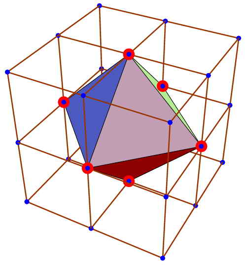
Figure 3: The momenta in the cubic lattice forming an orbit of length $6$ under the octahedral group are of the form $\{\pm n,0,0\}$, $\{0,\pm n,0\}$, $\{0,0,\pm n,\}$ and correspond to the vertices of a regular octahedron.

The complete classification of point orbits in the momentum lattice is organized as follows. First we subdivide the momenta into five groups:

A)

Momenta of type $\{a,0,0\}$ which generate $\mathrm{O_{24}}$ orbits of length 6 and representations of the universal group $\mathrm{G}_{1536}$ also of dimensions 6 (see fig.3).

B)

Momenta of type $\{a,a,a\}$ which generate $\mathrm{O_{24}}$ orbits of length 8 and representations of the universal group $\mathrm{G}_{1536}$ also of dimensions 8 (see fig.5).

C)

Momenta of type $\{a,a,0\}$ which generate $\mathrm{O_{24}}$ orbits of length 12 and representations of the universal group $\mathrm{G}_{1536}$ also of dimensions 12 (see fig4).

D)

Momenta of type $\{a,a,b\}$ which generate $\mathrm{O_{24}}$ orbits of length 24 and representations of the universal group $\mathrm{G}_{1536}$ also of dimensions 24 (see fig6).

E)

Momenta of type $\{a,b,c\}$ which generate $\mathrm{O_{24}}$ orbits of length 24 and representations of the universal group $\mathrm{G}_{1536}$ of dimensions 48.

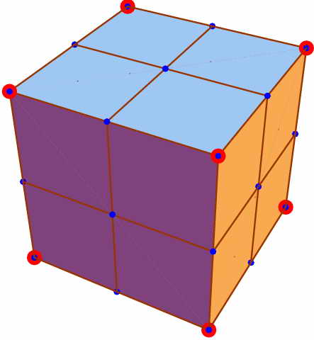
Figure 4: The momenta in the cubic lattice forming an orbit of length $8$ under the octahedral group are of the form $\{\pm n,\pm n,\pm n\}$, and correspond to the vertices of a regular cube.

The reason why in the cases A)…D) the dimension of the representation $\mathfrak{R}\left(\mathrm{\mathrm{G_{1536}}}\right)$ coincides with the dimension $|\mathcal{O}|$ of the orbit is simple. For each momentum in the orbit ($\forall\mathbf{k}_{i}\,\in\,\mathcal{O}$) also its negative is in the same orbit ($-\,\mathbf{k}_{i}\,\in\,\mathcal{O}$), hence the number of arguments $\Theta_{i}\,\equiv\,2\pi\,\mathbf{k}_{i}\cdot\mathbf{X}$ of the independent trigonometric functions $\sin\left(\Theta_{i}\right)$ and $\cos\left(\Theta_{i}\right)$ is ${\textstyle\frac{1}{2}}\times 2|\mathcal{O}|\,=\,|\mathcal{O}|$ since $\sin\left(\pm\Theta_{i}\right)\,=\,\pm\sin\left(\Theta_{i}\right)$ and $\cos\left(\pm\Theta_{i}\right)\,=\,\cos\left(\Theta_{i}\right)$.

In case E), instead, the negatives of all the members of the orbit $\mathcal{O}$ are not in $\mathcal{O}$. The number of independent trigonometric functions is therefore 48 and such is the dimension of the representation $\mathfrak{R}\left(\mathrm{\mathrm{G_{1536}}}\right)$.

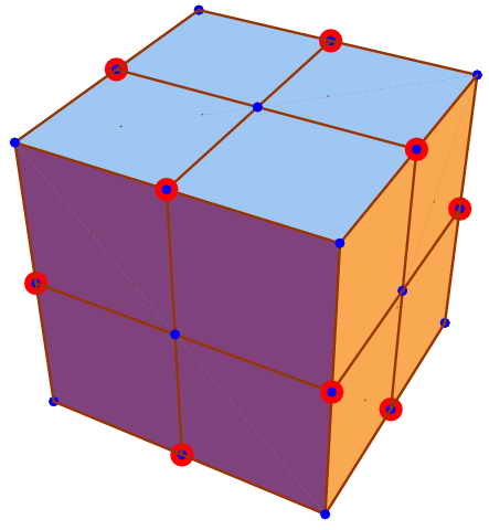
Figure 5: The momenta in the cubic lattice forming an orbit of length $12$ under the octahedral group are of the form $\{\pm n,\pm n,0\}$,$\{0,\pm n,\pm n\}$, $\{\pm n,0,\pm n\}$ and correspond to mid-points of the edges of a regular cube.

In each of the five groups one still has to reduce the entries to $\mathbb{Z}_{4}$, namely to consider their equivalence class $\mathrm{mod}\,4$. Each different choice of the pattern of $\mathbb{Z}_{4}$ classes appearing in an orbit leads to a different decomposition of the representation into irreducible representation of $\mathrm{G}_{1536}$. A simple consideration of the combinatorics leads to the conclusion that there are in total $48$ cases to be considered. The very significant result is that all of the $37$ irreducible representations of $\mathrm{G}_{1536}$ appear at least once in the list of these decompositions. Hence for all the irrepses of this group one can find a corresponding Beltrami field and for some irrepses such a Beltrami field admits a few inequivalent realizations. For the list of the $48$ distinct types of momentum vector classes and hence of Arnold Beltrami one-forms we refer the reader to [2].

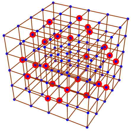
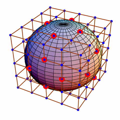
Figure 6: A view of an orbit of length 24 in the cubic lattice: the lattice points are of the form $\{\pm a,\pm a,\pm b\}$, $\{\pm a,\pm b,\pm a\}$,$\{\pm b,\pm a,\pm a\}$ and intersect the sphere of radius $r^{2}\,=\,2a^{2}+b^{2}$

4 The Discrete Group $\mathrm{GF_{192}}$

Among the various subgroups $\mathrm{H}\subset\mathrm{G_{1536}}$ that were listed in [2] and for which we provided there a full description together with their character tables, we have chosen a particular one, namely $\mathrm{GF_{192}}$ as our main token in order to illustrate by means of explicit examples the construction of $2$-brane solutions of $D=7$ supergravity. This choice is motivated by the fact that the Arnold-Beltrami one-forms extracted from the $6$-dimensional orbits of lattice momenta split into three-dimensional representations of this rather large space group. At the same time three-dimensional representations of the same space group occur also in the branching of other irreducible representations of $\mathrm{G_{1536}}$ generated by other type of momentum orbits, for instance by those of length $12$ (see [2] for more details). In this section we discuss the structure of this remarkable space group that, by means of supergravity, can be promoted to a discrete symmetry group of three-dimensional Maxwell–Chern–Simons gauge theories.

The precise definition of this group containing $192$-elements is provided in appendix A, where we list all of its elements, organized into 20 conjugacy classes. The nomenclature utilized to identify the elements is follows the notation introduced in eq.(2.75). An intrinsic description of the group can be given in terms of generators and relations. Let us choose the following three elements of the group:

$$\begin{array}[]{ccccc}S&=&\left\{4_{6},0,0,\frac{1}{2}\right\}&=&\left(\begin{array}[]{llllll}-\frac{1}{2}&\frac{1}{2}&0&-\frac{1}{2}&-\frac{1}{2}&0\\ \frac{1}{2}&\frac{1}{2}&0&-\frac{1}{2}&\frac{1}{2}&0\\ 0&0&-1&0&0&0\\ -\frac{1}{2}&-\frac{1}{2}&0&-\frac{1}{2}&\frac{1}{2}&0\\ -\frac{1}{2}&\frac{1}{2}&0&\frac{1}{2}&\frac{1}{2}&0\\ 0&0&0&0&0&1\end{array}\right)\\ Z&=&\left\{1_{1},0,0,1\right\}&=&\left(\begin{array}[]{llllll}0&0&0&-1&0&0\\ 0&0&0&0&-1&0\\ 0&0&1&0&0&0\\ -1&0&0&0&0&0\\ 0&-1&0&0&0&0\\ 0&0&0&0&0&1\end{array}\right)\\ T&=&\left\{2_{8},\frac{1}{2},\frac{3}{2},1\right\}&=&\left(\begin{array}[]{llllll}-\frac{1}{2}&-\frac{1}{2}&0&\frac{1}{2}&\frac{1}{2}&0\\ -\frac{1}{2}&0&\frac{1}{2}&-\frac{1}{2}&0&\frac{1}{2}\\ 0&-\frac{1}{2}&\frac{1}{2}&0&-\frac{1}{2}&-\frac{1}{2}\\ -\frac{1}{2}&\frac{1}{2}&0&\frac{1}{2}&-\frac{1}{2}&0\\ \frac{1}{2}&0&\frac{1}{2}&\frac{1}{2}&0&\frac{1}{2}\\ 0&\frac{1}{2}&\frac{1}{2}&0&\frac{1}{2}&-\frac{1}{2}\end{array}\right)\end{array}$$ (4.1)

where the $6\times 6$ representation is that provided by the $6\times 6$ defining representation of the parent group $\mathrm{G_{1536}}$. By direct evaluation on can verify that all elements of the group $\mathrm{GF_{192}}$ can be generated by multiple products of the generators (4.1). These latter satisfy the following relations

$$S^{2}\,=\,Z^{2}\,=\,T^{6} = \mathbf{1}$$

$$(S\,T)^{4}\,=\,(Z\,T)^{3}\,=\,(Z\,S)^{2} = \mathbf{1}$$ (4.2)

which can be taken as an intrinsic definition of the corresponding abstract group. The possibility of constructing all the irreducible representations of $\mathrm{GF_{192}}$ by means of an induction procedure is related with its solvability in terms of the following chain of normal subgroups:

$$\mathrm{GF_{192}}\,\rhd\,\mathrm{GF_{96}}\,\rhd\,\mathrm{GF_{48}}\,\rhd\,\mathrm{GF_{16}}$$ (4.3)

where the last element of the chain is abelian.

The group $\mathrm{G_{192}}$ has 20 conjugacy classes and therefore it has $20$ irreducible representations that are distributed according to the following pattern:

a)

4 irreps of dimension $1$, namely $\mathrm{D_{1},\dots,D_{4}}$

b)

12 irreps of dimension $3$, namely $\mathrm{D_{5},\dots,D_{16}}$

c)

2 irreps of dimension $2$, namely $\mathrm{D_{17},D_{18}}$

d)

2 irreps of dimension $6$, namely $\mathrm{D_{19},D_{20}}$

These representations were calculated in [2] to which we refer for further details. The character table is recalled below, where by $\epsilon$ we have denoted the cubic root of unity $\epsilon=\exp\left[\frac{2\pi}{3}\,{\rm i}\right]$.

$$\begin{array}[]{|l|llllllllllllllllllll|}\hline\cr 0&C_{1}&C_{2}&C_{3}&C_{4}&C_{5}&C_{6}&C_{7}&C_{8}&C_{9}&C_{10}&C_{11}&C_{12}&C_{13}&C_{14}&C_{15}&C_{16}&C_{17}&C_{18}&C_{19}&C_{20}\\ \hline\cr D_{1}&1&1&1&1&1&1&1&1&1&1&1&1&1&1&1&1&1&1&1&1\\ D_{2}&1&1&1&1&1&1&1&1&1&1&-1&-1&-1&-1&-1&-1&-1&-1&1&1\\ D_{3}&1&-1&-1&1&1&-1&1&-1&-1&1&1&-1&-1&1&1&-1&-1&1&1&-1\\ D_{4}&1&-1&-1&1&1&-1&1&-1&-1&1&-1&1&1&-1&-1&1&1&-1&1&-1\\ D_{5}&3&-3&-3&3&-1&1&-1&1&1&-1&-1&1&1&-1&1&-1&-1&1&0&0\\ D_{6}&3&-3&-3&3&-1&1&-1&1&1&-1&1&-1&-1&1&-1&1&1&-1&0&0\\ D_{7}&3&3&3&3&-1&-1&-1&-1&-1&-1&-1&-1&-1&-1&1&1&1&1&0&0\\ D_{8}&3&3&3&3&-1&-1&-1&-1&-1&-1&1&1&1&1&-1&-1&-1&-1&0&0\\ D_{9}&3&3&-1&-1&-1&3&3&-1&-1&-1&-1&1&-1&1&1&1&-1&-1&0&0\\ D_{10}&3&3&-1&-1&-1&3&3&-1&-1&-1&1&-1&1&-1&-1&-1&1&1&0&0\\ D_{11}&3&-3&1&-1&-1&-3&3&1&1&-1&-1&-1&1&1&1&-1&1&-1&0&0\\ D_{12}&3&-3&1&-1&-1&-3&3&1&1&-1&1&1&-1&-1&-1&1&-1&1&0&0\\ D_{13}&3&3&-1&-1&3&-1&-1&3&-1&-1&-1&1&-1&1&-1&-1&1&1&0&0\\ D_{14}&3&3&-1&-1&3&-1&-1&3&-1&-1&1&-1&1&-1&1&1&-1&-1&0&0\\ D_{15}&3&-3&1&-1&3&1&-1&-3&1&-1&-1&-1&1&1&-1&1&-1&1&0&0\\ D_{16}&3&-3&1&-1&3&1&-1&-3&1&-1&1&1&-1&-1&1&-1&1&-1&0&0\\ D_{17}&2&2&2&2&2&2&2&2&2&2&0&0&0&0&0&0&0&0&\epsilon(\epsilon+1)&\epsilon(\epsilon+1)\\ D_{18}&2&-2&-2&2&2&-2&2&-2&-2&2&0&0&0&0&0&0&0&0&\epsilon(\epsilon+1)&-\epsilon(\epsilon+1)\\ D_{19}&6&6&-2&-2&-2&-2&-2&-2&2&2&0&0&0&0&0&0&0&0&0&0\\ D_{20}&6&-6&2&-2&-2&2&-2&2&-2&2&0&0&0&0&0&0&0&0&0&0\\ \hline\cr\end{array}$$ (4.4)

The most attractive feature of this particular subgroup of the Universal Classifying group is given by the 12 three-dimensional representations $D_{5},\dots,D_{16}$. Any time we find one of these irreps in the decomposition with respect to $\mathrm{GF_{192}}$ of any of the 37 irreps of $\mathrm{G_{1536}}$, we can utilize the corresponding Arnold-Beltrami one-forms as fluxes in a $2$-brane solution of supergravity. Indeed in order to construct a solution of supergravity we are supposed to find an ansatz for the triplet of vector fields, $\mathbf{A}^{\Lambda}$ appearing in the bosonic spectrum of the theory. As we show in section 5.2, splitting the $7$ coordinates in a group of three spanning the brane world volume and a group of four $\{U,X,Y,Z\}$ transverse to the brane and further identifying the last three $\{X,Y,Z\}\equiv{\mathbf{X}}$ with those of a three torus $\mathrm{T^{3}}$, a convenient general ansatz is the following one:

$$\mathbf{A}^{\Lambda}\,=\,e^{2\,\mu\,U}\,\mathcal{E}^{\Lambda}_{\phantom{\Lambda}I}\,\mathbf{Y}^{I}({\mathbf{X}})$$ (4.5)

where $\mathbf{Y}^{A}({\mathbf{X}})$ is a basis set of solutions of Beltrami equation on the three-torus (2.23) with eigenvalue $\mu$ and $\mathcal{E}^{\Lambda}_{\phantom{\Lambda}I}$ is an embedding matrix ($3\times\mathrm{d}_{\mu}$) where $\mathrm{d}_{\mu}$ is the degeneracy of the eigenvalue $\mu$. The key point is that minimal $D=7$ supergravity has a global symmetry $\mathrm{SO(3)}$ with respect to which the triplet of vector fields transform in the defining three-dimensional representation. In the gauged version of the theory the same global symmetry $\mathrm{SO(3)}$ is promoted to a local one and the three vector fields become an $\mathrm{SO(3)}$-gauge connection. Consider now the action of a global discrete symmetry group $\Gamma$, like for instance $\mathrm{GF_{192}}$, on the Arnold-Beltrami one-forms $\mathbf{Y}^{I}({\mathbf{X}})$. We have:

$$\forall\,\gamma\,\in\,\Gamma\quad:\quad\mathbf{Y}^{I}(\,\gamma\cdot{\mathbf{X}})\,=\,\mathbf{Y}^{J}({\mathbf{X}})\,\mathrm{O}_{J}^{\phantom{J}I}(\gamma)\,$$ (4.6)

where, by an appropriate choice of the basis elements $\mathbf{Y}^{I}({\mathbf{X}})$ the matrix $\mathrm{O}^{I}_{\phantom{I}J}(\gamma)$ can always be made orthogonal:

$$\mathrm{O}(\gamma)\,\in\,\mathrm{O}(\mathrm{d}_{\mu})\quad\Rightarrow\quad\Gamma\,\subset\,\mathrm{O}(\mathrm{d}_{\mu})$$ (4.7)

As stressed in the above equation it follows that the discrete group $\Gamma$ is always a subgroup of the orthogonal group in a dimension equal to the multiplicity of the Beltrami eigenvalue. On the other hand $\Gamma\subset\mathrm{SO(3)}$, since all the considered $\Gamma$ have $3$-dimensional orthogonal representations. In this way the embedding matrix $\mathcal{E}^{\Lambda}_{\phantom{\Lambda}I}$ turns out to be an intertwining operator between irreducible representations of $\Gamma$. By Schur’s Lemma, there are only a few relevant type of cases:

$$\begin{array}[]{lcl}D_{x}(\Gamma,3)&\stackrel{{\scriptstyle\mathcal{E}}}{{\Leftrightarrow}}&D_{x}(\Gamma,3)\\ \left(\begin{array}[]{c|c}D_{x}(\Gamma,1)&0\\ \hline\cr 0&D_{y}(\Gamma,2)\\ \end{array}\right)&\stackrel{{\scriptstyle\mathcal{E}}}{{\Leftrightarrow}}&\left(\begin{array}[]{c|c}D_{x}(\Gamma,1)&0\\ \hline\cr 0&D_{y}(\Gamma,2)\\ \end{array}\right)\\ \left(\begin{array}[]{ccc}D_{x}(\Gamma,1)&0&0\\ 0&D_{y}(\Gamma,1)&0\\ 0&0&D_{z}(\Gamma,1)\\ \end{array}\right)&\stackrel{{\scriptstyle\mathcal{E}}}{{\Leftrightarrow}}&\left(\begin{array}[]{ccc}D_{x}(\Gamma,1)&0&0\\ 0&D_{y}(\Gamma,1)&0\\ 0&0&D_{z}(\Gamma,1)\\ \end{array}\right)\end{array}$$ (4.8)

where $\mathcal{E}$ intertwines between identical one-dimensional, two-dimensional and three-dimensional representations. Actually if we restrict our attention to cases that admit an uplifting to the gauged theory, the triplet representation of $\Gamma$ must be compatible with the adjoint of $\mathrm{SO(3)}$. Hence the only admitted cases are those where the final $3\times 3$ matrix has determinant one. The most natural choice is clearly that where $\mathcal{E}$ intertwines between two identical irreducible, faithful representations of $\Gamma$ and for this reason $\Gamma\,=\,\mathrm{GF_{192}}$ is an inspiring choice. It is a rather large subgroup of the Universal Classifying Group whose numerous irreducible three-dimensional representations are almost ubiquitous in all point orbit constructions of Arnold-Beltrami one-forms. For instance a quick survey of the branching rules presented in [2] and of the assignments to $\mathrm{G_{1536}}$-irreps of the Arnold-Beltrami one–forms constructed with point group orbits of lengths $6$, $8$ and $12$ (this information is also presented in [2]) reveals that using just only these type of momenta we can already construct triplets of Beltrami vector fields in the following eight irreducible three-dimensional representations of $\mathrm{GF_{192}}$: $\quad\mathrm{D_{5},D_{6},D_{7},D_{8},D_{9},D_{11},D_{13},D_{12},D_{12},D_{16}}$. In this paper we will not consider all such constructions neither we will attempt a classification of all $2$-brane solutions. We just confine ourselves to four examples that will illustrate the main features of this new playing ground for brane-physics.

4.1 A triplet of Arnold–Beltrami fields in the representation $\mathrm{D_{12}}\left[\mathrm{GF_{192}},3\right]$ from the octahedral orbit of ${\mathbf{k}}=\{1,0,0\}$

The first example that we consider corresponds to the celebrated ABC-flow that, in the hydrodynamical literature, has been the focus of many investigations over the last 40 years [3], [20].

According to the results of [2], if we construct the Arnold-Beltrami one-forms starting from the orbit of length six generated by the momentum ${\mathbf{k}}=\{1,0,0\}$, we obtain a set of 6 one–forms that transform in the representation $\mathrm{D_{23}}\left[\mathrm{G_{1536}},6\right]$ of the Universal Classifying Group. The branching rule of such a representation with respect to the considered subgroup $\mathrm{GF_{192}}$ is the following one:

$$\mathrm{D_{23}}\left[\mathrm{G_{1536}},6\right]\,=\,\mathrm{D_{12}}\left[\mathrm{GF_{192}},3\right]+\mathrm{D_{15}}\left[\mathrm{GF_{192}},3\right]$$ (4.9)

A generic one-form in the triplet representation $\mathrm{D_{12}}\left[\mathrm{GF_{192}},3\right]$ exactly corresponds to one of the ABC-flows, the parameters $\mathrm{A,B,C}$ being the components of a generic vector in this representation.

Projecting onto the representation $\mathrm{D_{12}}\left[\mathrm{GF_{192}},3\right]$ we find the following basis of one–forms:

$$\mathrm{D_{12}}\left[\mathrm{GF_{192}},3\right]\,\ni\,\mathbf{Y}^{I}\,=\,\left\{\begin{array}[]{rcl}\mathbf{Y}^{1}\left(X,Y,Z\right)&=&2\,\cos(2\pi Z)\mathrm{d}X-2\,\mathrm{d}Y\sin(2\pi Z)\\ \mathbf{Y}^{2}\left(X,Y,Z\right)&=&2\,\cos(2\pi Y)\mathrm{d}X+2\,\mathrm{d}Z\sin(2\pi Y))\\ \mathbf{Y}^{3}\left(X,Y,Z\right)&=&2\,\cos(2\pi X)\mathrm{d}Y-2\,\mathrm{d}Z\sin(2\pi X)\\ \end{array}\right.$$ (4.10)

that satisfy Beltrami equation with eigenvalue $\mu\,=\,2\pi$:

$$\star\,\mathrm{d}\mathbf{Y}^{I}\,=\,\mu\,\mathbf{Y}^{I}\quad;\quad\mu\,=\,2\pi\,\sqrt{\mathbf{k}\cdot\mathbf{k}}\,=\,\,2\pi$$ (4.11)

The components of these one–forms are easily extracted utilizing the definition:

$$\mathbf{Y}^{I}\,=\,\mathbf{Y}^{I}_{i}\,\mathrm{d}X^{i}\quad;\quad\mathrm{d}X^{i}\,=\,\left\{\mathrm{d}X,\mathrm{d}Y,\mathrm{d}Z\right\}$$ (4.12)

and the explicit action of the $\mathrm{GF_{192}}$ group on these one-forms is specified once we give the explicit action of the three generators $S,Z,T$. This latter is the following one:

$$\begin{array}[]{rccclcccc}S&:&\{X,Y,Z\}&\to&\left\{Y,X,\frac{1}{4}-Z\right\}&\Rightarrow&\mathrm{D_{12}}[S]&=&\left(\begin{array}[]{lll}-1&0&0\\ 0&0&1\\ 0&1&0\end{array}\right)\\ \hbox{}\hfil&\hbox{}\hfil&\hbox{}\hfil&\hbox{}\hfil&\hbox{}&\hbox{}\hfil&\hbox{}\hfil&\hbox{}\hfil&\hbox{}\hfil\\ Z&:&\{X,Y,Z\}&\to&\left\{X,Y,Z+\frac{1}{2}\right\}&\Rightarrow&\mathrm{D_{12}[Z]}&=&\left(\begin{array}[]{lll}-1&0&0\\ 0&1&0\\ 0&0&1\end{array}\right)\\ \hbox{}\hfil&\hbox{}\hfil&\hbox{}\hfil&\hbox{}\hfil&\hbox{}&\hbox{}\hfil&\hbox{}\hfil&\hbox{}\hfil&\hbox{}\hfil\\ T&:&\{X,Y,Z\}&\to&\left\{Y+\frac{1}{4},Z+\frac{3}{4},X+\frac{1}{2}\right\}&\Rightarrow&\mathrm{D_{12}}[T]&=&\left(\begin{array}[]{lll}0&-1&0\\ 0&0&-1\\ -1&0&0\end{array}\right)\end{array}$$ (4.13)

$$\mathbf{Y}\left(Y,X,\frac{1}{4}-Z\right) = \mathbf{Y}\left(X,Y,Z\right)\cdot\mathrm{D_{12}}[S]$$

$$\mathbf{Y}\left(X,Y,Z+\frac{1}{2}\right) = \mathbf{Y}\left(X,Y,Z\right)\cdot\mathrm{D_{12}}[Z]$$

$$\mathbf{Y}\left(Y+\frac{1}{4},Z+\frac{3}{4},X+\frac{1}{2}\right) = \mathbf{Y}\left(X,Y,Z\right)\cdot\mathrm{D_{12}}[T]$$ (4.14)

Next we calculate the matrix of scalar products of the basis one-forms:

$$gY^{IJ}\,\equiv\,\langle\mathbf{Y}^{I}\,,\,\mathbf{Y}^{J}\rangle\,\equiv\,\sum_{i=1}^{3}\,\mathbf{Y}^{I}_{i}\mathbf{Y}^{J}_{i}$$ (4.15)

and we find:

$$gY^{IJ}\,=\,\left(\begin{array}[]{lll}4&4\cos(2\pi Y)\cos(2\pi Z)&-4\cos(2\pi X)\sin(2\pi Z)\\ 4\cos(2\pi Y)\cos(2\pi Z)&4&-4\sin(2\pi X)\sin(2\pi Y)\\ -4\cos(2\pi X)\sin(2\pi Z)&-4\sin(2\pi X)\sin(2\pi Y)&4\end{array}\right)$$ (4.16)

The trace of this matrix, which plays an important role in the $2$-brane construction is in this case a constant:

$$\mbox{Tr}\left(gY_{IJ}\right) \equiv \Lambda_{\mathbf{1,0,0}}^{\mathrm{D_{12}}(\mathrm{GF_{192}},3)}\,+\,\mathfrak{J}_{\mathbf{1,0,0}}^{\mathrm{D_{12}}(\mathrm{GF_{192}},3)}\left(X,Y,Z\right)$$

$$\Lambda_{\mathbf{1,0,0}}^{\mathrm{D_{12}}(\mathrm{GF_{192}},3)} = 12$$

$$\mathfrak{J}_{\mathbf{1,0,0}}^{\mathrm{D_{12}}(\mathrm{GF_{192}},3)}\left(X,Y,Z\right) = 0$$ (4.17)

4.2 A singlet of Arnold–Beltrami fields in the representation $\mathrm{D_{1}}\left[\mathrm{GS_{24}},1\right]$ from the octahedral orbit of ${\mathbf{k}}=\{1,0,0\}$

The second example that we consider corresponds to the case of the AAA-flow, namely to the subcase of the ABC-flows that is invariant under the subgroup $\mathrm{GS_{24}}\subset\mathrm{GF_{192}}$. As explained in [2], under the subgroup $\mathrm{GS_{24}}$, which is isomorphic to the octahedral group and is thoroughly described in appendix A.2, the irreducible representation $\mathrm{D_{12}}(\mathrm{GF_{192}},3)$ branches as follows:

$$\mathrm{D_{12}}(\mathrm{GF_{192}},3)\,=\,\mathrm{D_{1}}(\mathrm{GS_{24}},1)\oplus\mathrm{D_{3}}(\mathrm{GS_{24}},2)$$ (4.18)

This means that from the construction considered in section 4.1 of Arnold-Beltrami fields associated with the orbit of the momentum vector ${\mathbf{k}}=\{1,0,0\}$, we can extract a vector field that is in the singlet representation of $\mathrm{GS_{24}}$.

Projecting onto this singlet, according with eq.(4.8) we obtain the following basis of one–forms:

$$\mathrm{D_{1}}\left[\mathrm{GS_{24}},1\right]\,\ni\,\mathbf{Y}^{I}\,=\,\left\{\begin{array}[]{rcl}\mathbf{Y}^{1}\left(X,Y,Z\right)&=&2{dY}\cos[2\pi X]+2{dX}\cos[2\pi Y]+2{dX}\cos[2\pi Z]\\ &&-2{dZ}\sin[2\pi X]+2{dZ}\sin[2\pi Y]-2{dY}\sin[2\pi Z]\\ \mathbf{Y}^{2}\left(X,Y,Z\right)&=&0\\ \mathbf{Y}^{3}\left(X,Y,Z\right)&=&0\\ \end{array}\right.$$ (4.19)

satisfying Beltrami equation with eigenvalue $\mu\,=\,2\pi$:

$$\star\,\mathrm{d}\mathbf{Y}^{I}\,=\,\mu\,\mathbf{Y}^{I}\quad;\quad\mu\,=\,2\pi\,\sqrt{\mathbf{k}\cdot\mathbf{k}}\,=\,\,2\pi$$ (4.20)

The components of these one–forms are easily extracted utilizing the definition:

$$\mathbf{Y}^{I}\,=\,\mathbf{Y}^{I}_{i}\,\mathrm{d}X^{i}\quad;\quad\mathrm{d}X^{i}\,=\,\left\{\mathrm{d}X,\mathrm{d}Y,\mathrm{d}Z\right\}$$ (4.21)

The explicit action of the $\mathrm{GS_{24}}$ group on these one-forms is specified once we give the explicit action of the two generators $S,T$, satisfying the defining relations:

$$S^{2}\,=\,T^{3}\,=\,(S\,T)^{4}\,=\,\mathbf{e}$$ (4.22)

Two such generators can be chosen as follows:

$$S \equiv \left\{4_{6},0,0,\frac{3}{2}\right\}$$ (4.23)

$$T \equiv \left\{2_{8},\frac{3}{2},\frac{1}{2},0\right\}$$ (4.24)

The action of these latter is the following one:

$$\begin{array}[]{rccclcccc}S&:&\{X,Y,Z\}&\to&\left\{Y,X,\frac{3}{4}-Z\right\}&\Rightarrow&\mathrm{D_{1}}[S]&=&1\\ \hbox{}\hfil&\hbox{}\hfil&\hbox{}\hfil&\hbox{}\hfil&\hbox{}&\hbox{}\hfil&\hbox{}\hfil&\hbox{}\hfil&\hbox{}\hfil\\ T&:&\{X,Y,Z\}&\to&\left\{Y+\frac{3}{4},Z+\frac{1}{4},X\right\}&\Rightarrow&\mathrm{D_{1}}[T]&=&1\\ \end{array}$$ (4.25)

$$\mathbf{Y}\left(Y,X,\frac{3}{4}-Z\right) = \mathbf{Y}\left(X,Y,Z\right)$$

$$\mathbf{Y}\left(Y+\frac{3}{4},Z+\frac{1}{4},X\right) = \mathbf{Y}\left(X,Y,Z\right)$$ (4.26)

Next we calculate the matrix of scalar products of the basis one-forms:

$$gY^{IJ}\,\equiv\,\langle\mathbf{Y}^{I}\,,\,\mathbf{Y}^{J}\rangle\,\equiv\,\sum_{i=1}^{3}\,\mathbf{Y}^{I}_{i}\mathbf{Y}^{J}_{i}$$ (4.27)

and we find:

$$gY^{IJ}\,=\,\left(\begin{array}[]{ccc}\Lambda_{\mathbf{1,0,0}}^{\mathrm{D_{1}}(\mathrm{GS_{24}},1)}\,+\,\mathfrak{J}_{\mathbf{1,0,0}}^{\mathrm{D_{1}}(\mathrm{GS_{24}},1)}\left(X,Y,Z\right)&0&0\\ 0&0&0\\ 0&0&0\end{array}\right)$$ (4.28)

The trace of this matrix, which plays an important role in the $2$-brane construction is obviously equal to the first and unique non vanishing element of the matrix (4.28):

$$\mbox{Tr}\left(gY_{IJ}\right) \equiv \Lambda_{\mathbf{1,0,0}}^{\mathrm{D_{1}}(\mathrm{GS_{24}},1)}\,+\,\mathfrak{J}_{\mathbf{1,0,0}}^{\mathrm{D_{1}}(\mathrm{GS_{24}},1)}\left(X,Y,Z\right)$$

$$\Lambda_{\mathbf{1,0,0}}^{\mathrm{D_{1}}(\mathrm{GS_{24}},1)} = 12$$ (4.29)

$$\mathfrak{J}_{\mathbf{1,0,0}}^{\mathrm{D_{1}}(\mathrm{GS_{24}},1)}\left(X,Y,Z\right) = -4\cos[2\pi(X-Y)]+4\cos[2\pi(X+Y)]+4\cos[2\pi(Y-Z)]$$ (4.30)

$$+4\cos[2\pi(Y+Z)]+4\sin[2\pi(X-Z)]-4\sin[2\pi(X+Z)]$$

Defining the three-dimensional Laplacian:

$$\Delta_{\mathrm{T^{3}}}\,\equiv\,\frac{\partial^{2}}{\partial X^{2}}\,+\,\frac{\partial^{2}}{\partial Y^{2}}\,+\,\frac{\partial^{2}}{\partial Z^{2}}$$ (4.31)

we can verify that the function $\mathfrak{J}_{\mathbf{1,0,0}}^{\mathrm{D_{1}}(\mathrm{GS_{24}},1)}\left(X,Y,Z\right)$ defined in eq.(4.30) is invariant under the full group $\mathrm{GS_{24}}$ and that it is an eigenfunction of $\Delta_{\mathrm{T^{3}}}$ with eigenvalue $\lambda\,=\,-\,2\,\mu^{2}$:

$$\Delta_{\mathrm{T^{3}}}\,\mathfrak{J}_{\mathbf{1,0,0}}^{\mathrm{D_{1}}(\mathrm{GS_{24}},1)}\left(X,Y,Z\right)\,=\,\lambda\,\mathfrak{J}_{\mathbf{1,0,0}}^{\mathrm{D_{1}}(\mathrm{GS_{24}},1)}\left(X,Y,Z\right)\quad;\quad\lambda\,=\,-\,8\pi^{2}\,=\,-\,2\,\mu^{2}$$ (4.32)

4.3 A triplet of Arnold–Beltrami fields in the representation $\mathrm{D_{7}}\left[\mathrm{GF_{192}},3\right]$ from the octahedral orbit of ${\mathbf{k}}=\{2,0,0\}$

The third example that we consider is extracted from the orbit of length six generated by the momentum ${\mathbf{k}}=\{2,0,0\}$. From this construction we obtain a set of six one–forms that transform in the representation $\mathrm{D_{19}}\left[\mathrm{G_{1536}},6\right]$ of the Universal Classifying Group. As given in [2], the branching rule of such a representation with respect to the considered subgroup $\mathrm{GF_{192}}$ is the following one:

$$\mathrm{D_{19}}\left[\mathrm{G_{1536}},6\right]\,=\,\mathrm{D_{7}}\left[\mathrm{GF_{192}},3\right]+\mathrm{D_{8}}\left[\mathrm{GF_{192}},3\right]$$ (4.33)

Projecting onto the representation $\mathrm{D_{7}}\left[\mathrm{GF_{192}},3\right]$ we find the following basis of one–forms:

$$\mathrm{D_{7}}\left[\mathrm{GF_{192}},3\right]\,\ni\,\mathbf{Y}^{I}\,=\,\left\{\begin{array}[]{rcl}\mathbf{Y}^{1}\left(X,Y,Z\right)&=&2(\cos(4\pi Y)+\cos(4\pi Z))\mathrm{d}X+2\mathrm{d}Z\sin(4\pi Y)-2\mathrm{d}Y\sin(4\pi Z)\\ \mathbf{Y}^{2}\left(X,Y,Z\right)&=&2(\cos(4\pi X)-\cos(4\pi Z))\mathrm{d}Y-2(\mathrm{d}Z\sin(4\pi X)+\mathrm{d}X\sin(4\pi Z))\\ \mathbf{Y}^{3}\left(X,Y,Z\right)&=&2(\cos(4\pi X)+\cos(4\pi Y))\mathrm{d}Z+2\mathrm{d}Y\sin(4\pi X)-2\mathrm{d}X\sin(4\pi Y)\\ \end{array}\right.\\$$

that satisfy Beltrami equation with eigenvalue $\mu\,=\,4\pi$:

$$\star\,\mathrm{d}\mathbf{Y}^{I}\,=\,\mu\,\mathbf{Y}^{I}\quad;\quad\mu\,=\,2\pi\,\sqrt{\mathbf{k}\cdot\mathbf{k}}\,=\,\,4\pi$$ (4.34)

The components of these one–forms are easily extracted from:

$$\mathbf{Y}^{I}\,=\,\mathbf{Y}^{I}_{i}\,\mathrm{d}X^{i}\quad;\quad\mathrm{d}X^{i}\,=\,\left\{\mathrm{d}X,\mathrm{d}Y,\mathrm{d}Z\right\}$$ (4.35)

In this representation the explicit action of the three generators $S,Z,T$ is the following one:

$$\begin{array}[]{rccclcccc}S&:&\{X,Y,Z\}&\to&\left\{Y,X,\frac{1}{4}-Z\right\}&\Rightarrow&\mathrm{D_{7}}[S]&=&\left(\begin{array}[]{lll}0&1&0\\ 1&0&0\\ 0&0&-1\end{array}\right)\\ \hbox{}\hfil&\hbox{}\hfil&\hbox{}\hfil&\hbox{}\hfil&\hbox{}&\hbox{}\hfil&\hbox{}\hfil&\hbox{}\hfil&\hbox{}\hfil\\ Z&:&\{X,Y,Z\}&\to&\left\{X,Y,Z+\frac{1}{2}\right\}&\Rightarrow&\mathrm{D_{7}[Z]}&=&\left(\begin{array}[]{lll}1&0&0\\ 0&1&0\\ 0&0&1\end{array}\right)\\ \hbox{}\hfil&\hbox{}\hfil&\hbox{}\hfil&\hbox{}\hfil&\hbox{}&\hbox{}\hfil&\hbox{}\hfil&\hbox{}\hfil&\hbox{}\hfil\\ T&:&\{X,Y,Z\}&\to&\left\{Y+\frac{1}{4},Z+\frac{3}{4},X+\frac{1}{2}\right\}&\Rightarrow&\mathrm{D_{7}}[T]&=&\left(\begin{array}[]{lll}0&0&-1\\ 1&0&0\\ 0&-1&0\end{array}\right)\end{array}$$ (4.36)

and we have:

$$\mathbf{Y}\left(Y,X,\frac{1}{4}-Z\right) = \mathbf{Y}\left(X,Y,Z\right)\cdot\mathrm{D_{7}}[S]$$

$$\mathbf{Y}\left(X,Y,Z+\frac{1}{2}\right) = \mathbf{Y}\left(X,Y,Z\right)\cdot\mathrm{D_{7}}[Z]$$

$$\mathbf{Y}\left(Y+\frac{1}{4},Z+\frac{3}{4},X+\frac{1}{2}\right) = \mathbf{Y}\left(X,Y,Z\right)\cdot\mathrm{D_{7}}[T]$$ (4.37)

Next we calculate the matrix of scalar products of the basis one-forms:

$$gY^{IJ}\,\equiv\,\langle\mathbf{Y}^{I}\,,\,\mathbf{Y}^{J}\rangle\,\equiv\,\sum_{i=1}^{3}\,\mathbf{Y}^{I}_{i}\mathbf{Y}^{J}_{i}$$ (4.38)

We do not display this matrix since it is too large, but we write its trace which is the most important item entering the $2$-brane construction.

$$\mbox{Tr}\left(gY_{IJ}\right) \equiv \Lambda_{\mathbf{2,0,0}}^{\mathrm{D_{7}}(\mathrm{GF_{192}},3)}\,+\,\mathfrak{J}_{\mathbf{2,0,0}}^{\mathrm{D_{7}}(\mathrm{GF_{192}},3)}\left(X,Y,Z\right)$$

$$\Lambda_{\mathbf{2,0,0}}^{\mathrm{D_{7}}(\mathrm{GF_{192}},3)} = 24$$

$$\mathfrak{J}_{\mathbf{2,0,0}}^{\mathrm{D_{7}}(\mathrm{GF_{192}},3)}\left(X,Y,Z\right) = 8\left(\cos[4\pi X]\left(\cos[4\pi Y]-\cos[4\pi Z]\right)+\cos[4\pi Y]\cos[4\pi Z]\right)$$ (4.39)

Then we can verify that the function $\mathfrak{J}_{\mathbf{2,0,0}}^{\mathrm{D_{7}}(\mathrm{GF_{192}},3)}\left(X,Y,Z\right)$ is invariant under the full group $\mathrm{GF_{192}}$ and that it is an eigenfunction of $\Delta_{\mathrm{T^{3}}}$ with eigenvalue $\lambda\,=\,-\,2\,\mu^{2}$:

$$\Delta_{\mathrm{T^{3}}}\,\mathfrak{J}_{\mathbf{2,0,0}}^{\mathrm{D_{7}}(\mathrm{GF_{192}},3)}\left(X,Y,Z\right)\,=\,\lambda\,\mathfrak{J}_{\mathbf{2,0,0}}^{\mathrm{D_{7}}(\mathrm{GF_{192}},3)}\left(X,Y,Z\right)\quad;\quad\lambda\,=\,-\,32\pi^{2}\,=\,-\,2\,\mu^{2}$$ (4.40)

4.4 A triplet of Arnold–Beltrami fields in the representation $\mathrm{D_{9}}\left[\mathrm{GF_{192}},3\right]$ from the octahedral orbit of ${\mathbf{k}}=\{1,1,0\}$

The third example that we consider is extracted from the orbit of length twelve generated by the momentum ${\mathbf{k}}=\{1,1,0\}$. From this construction we obtain a set of 12 one–forms that transform in the representation $\mathrm{D_{32}}\left[\mathrm{G_{1536}},6\right]$ of the Universal Classifying Group. According to [2], the branching rule of such a representation with respect to the considered subgroup $\mathrm{GF_{192}}$ is the following one:

$$\mathrm{D_{32}}\left[\mathrm{G_{1536}},6\right]\,=\,\mathrm{D_{9}}\left[\mathrm{GF_{192}},3\right]+\mathrm{D_{13}}\left[\mathrm{GF_{192}},3\right]+\mathrm{D_{19}}\left[\mathrm{GF_{192}},6\right]$$ (4.41)

Projecting onto the representation $\mathrm{D_{9}}\left[\mathrm{GF_{192}},3\right]$ we find the following basis of one–forms:

$$\mathbf{Y}^{I}\left(X,Y,Z\right) \in \mathrm{D_{9}}\left[\mathrm{GF_{192}},3\right]$$

$$\mathbf{Y}^{1}\left(X,Y,Z\right) = \sqrt{2}\Big{(}\left(\mathrm{d}Z-\mathrm{d}Y\right)\sin[2\pi(Y+Z)]-\left(\mathrm{d}Y+\mathrm{d}Z\right)\sin[2\pi(Y-Z)]\Big{)}-4\,\mathrm{d}X\sin[2\pi Y]\sin[2\pi Z]$$

$$\mathbf{Y}^{2}\left(X,Y,Z\right) = \sqrt{2}\Big{(}\sqrt{2}\left(\left(-\mathrm{d}Y-\mathrm{d}Z\right)\sin[2\pi(Y-Z)]+\left(\mathrm{d}Z-\mathrm{d}Y\right)\sin[2\pi(Y+Z)]\right)$$

$$-4\,\mathrm{d}X\sin[2\pi Y]\sin[2\pi Z]\Big{)}$$

$$\mathbf{Y}^{3}\left(X,Y,Z\right) = \sqrt{2}\Big{(}\,2\,\mathrm{d}Z\,(\cos[2\pi(X-Y)]+\cos[2\pi(X+Y)])\,$$

$$+\sqrt{2}((\mathrm{d}X+\mathrm{d}Y)\sin[2\pi(X-Y)]+(\mathrm{d}Y-\mathrm{d}X)\sin[2\pi(X+Y)])\Big{)}$$

that satisfy Beltrami equation with eigenvalue $\mu\,=\,2\sqrt{2}\pi$:

$$\star\,\mathrm{d}\mathbf{Y}^{I}\,=\,\mu\,\mathbf{Y}^{I}\quad;\quad\mu\,=\,2\pi\,\sqrt{\mathbf{k}\cdot\mathbf{k}}\,=\,\,2\sqrt{2}\pi$$ (4.43)

The components of these one–forms are easily extracted from:

$$\mathbf{Y}^{I}\,=\,\mathbf{Y}^{I}_{i}\,\mathrm{d}X^{i}\quad;\quad\mathrm{d}X^{i}\,=\,\left\{\mathrm{d}X,\mathrm{d}Y,\mathrm{d}Z\right\}$$ (4.44)

In this representation the explicit action of the three generators $S,Z,T$ is the following one:

$$\begin{array}[]{rccclcccc}S&:&\{X,Y,Z\}&\to&\left\{Y,X,\frac{1}{4}-Z\right\}&\Rightarrow&\mathrm{D_{9}}[S]&=&\left(\begin{array}[]{lll}0&-\frac{1}{2}&0\\ -2&0&0\\ 0&0&-1\end{array}\right)\\ \hbox{}\hfil&\hbox{}\hfil&\hbox{}\hfil&\hbox{}\hfil&\hbox{}&\hbox{}\hfil&\hbox{}\hfil&\hbox{}\hfil&\hbox{}\hfil\\ Z&:&\{X,Y,Z\}&\to&\left\{X,Y,Z+\frac{1}{2}\right\}&\Rightarrow&\mathrm{D_{9}[Z]}&=&\left(\begin{array}[]{lll}-1&0&0\\ 0&-1&0\\ 0&0&1\end{array}\right)\\ \hbox{}\hfil&\hbox{}\hfil&\hbox{}\hfil&\hbox{}\hfil&\hbox{}&\hbox{}\hfil&\hbox{}\hfil&\hbox{}\hfil&\hbox{}\hfil\\ T&:&\{X,Y,Z\}&\to&\left\{Y+\frac{1}{4},Z+\frac{3}{4},X+\frac{1}{2}\right\}&\Rightarrow&\mathrm{D_{9}}[T]&=&\left(\begin{array}[]{lll}0&-\frac{1}{2}&0\\ 0&0&1\\ -2&0&0\end{array}\right)\end{array}$$ (4.45)

and we have:

$$\mathbf{Y}\left(Y,X,\frac{1}{4}-Z\right) = \mathbf{Y}\left(X,Y,Z\right)\cdot\mathrm{D_{9}}[S]$$

$$\mathbf{Y}\left(X,Y,Z+\frac{1}{2}\right) = \mathbf{Y}\left(X,Y,Z\right)\cdot\mathrm{D_{9}}[Z]$$

$$\mathbf{Y}\left(Y+\frac{1}{4},Z+\frac{3}{4},X+\frac{1}{2}\right) = \mathbf{Y}\left(X,Y,Z\right)\cdot\mathrm{D_{9}}[T]$$ (4.46)

Next we calculate the matrix of scalar products of the basis one-forms:

$$gY^{IJ}\,\equiv\,\langle\mathbf{Y}^{I}\,,\,\mathbf{Y}^{J}\rangle\,\equiv\,\sum_{i=1}^{3}\,\mathbf{Y}^{I}_{i}\mathbf{Y}^{J}_{i}$$ (4.47)

We do not display this matrix since it is too large, but we write its trace which is the most important item entering the $2$-brane construction:

$$\mbox{Tr}\left(gY_{IJ}\right) \equiv \Lambda_{\mathbf{1,1,0}}^{\mathrm{D_{9}}(\mathrm{GF_{192}},3)}\,+\,\mathfrak{J}_{\mathbf{1,1,0}}^{\mathrm{D_{9}}(\mathrm{GF_{192}},3)}\left(X,Y,Z\right)$$

$$\Lambda_{\mathbf{1,1,0}}^{\mathrm{D_{9}}(\mathrm{GF_{192}},3)} = 48$$

$$\mathfrak{J}_{\mathbf{1,1,0}}^{\mathrm{D_{9}}(\mathrm{GF_{192}},3)}\left(X,Y,Z\right) = 0$$ (4.48)

5 D=7 two-branes with Arnold Beltrami Fluxes in the transverse directions

After the long preparation of the previous sections we can finally come to the central issue addressed in the present paper, namely the construction of two-brane solutions of $D=7$ minimal supergravity with Arnold-Beltrami fluxes in the transverse space. Initially, without making direct reference to supergravity, we consider the general form of a $p$-brane action as it is described in many places in the literature and we focus on the the case $p\,=\,2$ in $D=7$. Our first concern is the elementary $2$-brane solution in $D=7$. We show that this latter exists for all values of the exponential coupling parameter $a$ whose definition is recalled below. Each value of $a$ corresponds to a different value of the dimensional reduction invariant parameter $\Delta$ whose definition is also recalled below. Obviously $D=7$ supergravity corresponds to a unique value of $\Delta$ which can be determined by comparing the general brane-action with the bosonic action of minimal $D=7$ supergravity, as it was constructed in the original papers of thirty years ago, namely in [9] and [11]. It turns out that for supergravity the value of $\Delta$ is the magic one $\Delta\,=\,4$ for which the solution becomes particularly simple and elegant and typically preserves one half of the supersymmetries.

Subsequently, on the background of the $2$-brane solution we switch on fluxes of an additional triplet of vector fields, in this way completing the bosonic field content of minimal $D=7$ supergravity. In presence of a topological interaction term between the triplet of gauge fields and the $3$-form which defines the $2$-brane, we show that the additional fluxes can be fitted into the framework of an exact solution if they are Arnold Beltrami vector fields satisfying Beltrami equation (2.23). The only conditions for the existence of such a solution is $\Delta\,=\,4$ plus a precise relation between the coefficients of the kinetic terms in the lagrangian and the coefficient of the topological interaction term. Clearly we expect that such a relation should be satisfied by the coefficients of minimal $D=7$ supergravity and by comparison with [9],[11], it is shown that this is indeed the case. Thus we arrive at the very much inspiring conclusion that $2$-branes with Arnold-Beltrami fluxes in the transverse space are just a special feature of minimal $D=7$ supergravity. Deriving the number of Killing spinors possessed by each solution, analyzing the relation of these latter with the discrete symmetry groups introduced by the AB-fluxes and establishing the corresponding Maxwell-Chern-Simons gauge theories on the world volume are obviously the next steps in a vast programme of investigations that opens up as a consequence of the result we present here.

In order to accomplish this programme we need a firm control on the Lagrangian and the supersymmetry transformation rules of this remarkable supergravity, both in its gauged and in its ungauged versions. For this reason, within the framework of a larger collaboration [24], we have started a thorough reconstruction of minimal $D=7$ supergravity in the rheonomic approach [25] and the result of this reconstruction will form the framework for our further investigation of $2$-branes with Arnold-Beltrami fluxes.

5.1 The general form of a $2$-brane action in $D=7$

In the mostly minus metric that we utilize, the correct form of the action in $D=7$ admitting an electric $2$-brane solution is the following one:

$$\mathcal{A}_{2brane} = \int\,d^{7}x\,\mathcal{L}_{2brane}$$

$$\mathcal{L}_{2brane} = \mbox{det}V\,\left(-R[g]\,-\,{\textstyle\frac{1}{4}}\,\partial^{\mu}\varphi\,\partial_{\mu}\varphi\,+\,{\textstyle\frac{1}{96}}\,e^{-a\,\varphi}\,\mathbf{F}_{\lambda\mu\nu\rho}\,\mathbf{F}^{\lambda\mu\nu\rho}\right)$$ (5.1)

where $a$ is a free parameter, $\varphi$ denotes the dilaton field with a canonically normalized kinetic term and :

$$\mathbf{F}_{\lambda\mu\nu\rho}\,\equiv\,\partial_{[\lambda}\,\mathbf{A}_{\mu\nu\rho]}$$ (5.2)

is the field-strength of the three-form $\mathbf{A}^{[3]}$ which couples to the world volume of the two-brane.

The field equations following from (5.1) can be put into the following convenient form:

$$\Box_{cov}\,\varphi = \frac{a}{48}e^{-a\varphi}\,\mathbf{F}_{\lambda\mu\nu\rho}\,\mathbf{F}^{\lambda\mu\nu\rho}$$ (5.3)

$$\mathrm{d}\star\left[e^{-a\varphi}\,\star\mathbf{F}^{[4]}\right] = 0$$ (5.4)

$$\mbox{Ric}_{\mu\nu} = \frac{1}{4}\partial_{\mu}\varphi\,\partial_{\nu}\varphi\,+\,S_{\mu\nu}$$ (5.5)

$$S_{\mu\nu} = -\,\frac{1}{24}e^{-a\varphi}\left(\mathbf{F}_{\mu...}\,\mathbf{F}_{\nu}^{\phantom{\nu}...}\,-\,{\textstyle\frac{3}{20}}\,g_{\mu\nu}\,\mathbf{F}_{....}\,\mathbf{F}^{....}\right)$$ (5.6)

and they admit the following exact electric $2$-brane solution:

$$ds^{2} = H(y)^{-\frac{8}{5\Delta}}\,d\xi^{\mu}\otimes d\xi^{\nu}\,-\,H(y)^{\frac{12}{5\Delta}}\,dy^{I}\otimes dy^{J}\,\delta_{IJ}$$

$$\phi = -\frac{2a}{\Delta}\,\log\,H(y)$$

$$\mathbf{F}_{[4]} = \mathrm{d}\left[H(y)^{-1}\,\frac{1}{3!}\,\mathrm{d}\xi^{\mu}\wedge\mathrm{d}\xi^{\nu}\wedge\mathrm{d}\xi^{\rho}\,\epsilon_{\mu\nu\rho}\right]$$ (5.7)

where, according to the main idea put forward in the introduction (see fig.1) the seven coordinates have been separated into two sets, the first set of three $\xi^{\mu}$ ($\mu=0,1,2$) spanning the $2$-brane world volume, the second set of four $y^{I}$ ($I=3,4,5,6$) spanning the transverse space to the brane. In the above solution $H(y)$ is any harmonic function living on the $4$-dimensional transverse space to the brane whose metric is assumed to be flat:

$$\Box_{\mathbb{R}^{4}}\,H(y)\,\equiv\,\sum_{I=1}^{4}\frac{\partial^{2}}{\partial(y^{I})^{2}}H(y)\,=\,0$$ (5.8)

and the parameters $a$ and $\Delta$ are related by the celebrated formula:

$$\Delta\,=\,a^{2}\,+\,2\frac{d\,\widetilde{d}}{D-2}\,=\,a^{2}\,+\,\frac{12}{5}$$ (5.9)

which follows from $d=3,\quad\widetilde{d}\,=\,2$ and $D=7$. Physically $d$ is the dimension of the electric $2$-brane world volume, while $\widetilde{d}$ is the dimension of the world-sheet spanned by the magnetic string which is dual to the $2$-brane.

In section 6 we will discuss the relation of the brane action (5.1) with the bosonic action of minimal ungauged $D=7$ supergravity and show that the specific coefficients of the kinetic terms appearing in this latter determine the value of $\Delta$. Indeed the supersymmetry of the action imposes $\Delta\,=\,4$. In a future publication [24], after the rheonomic reconstruction of the theory is completed we will discuss the Killing spinors admitted by the solution (5.7) and by its extension with Arnold-Beltrami fluxes.

5.2 The two-brane with Arnold Beltrami Fluxes

As a next step we generalize the two-brane action (5.1) introducing also a triplet of one-form fields $\mathbf{A}^{\Lambda}$, ($\Lambda\,=\,1,2,3$) whose field strengths we denote $\mathbf{F}^{\Lambda}\,\equiv\,\mathrm{d}\mathbf{A}^{\Lambda}$. In this way we complete the field-content of minimal $D=7$ supergravity. Explicitly we write the new bosonic action:

$$\mathcal{A}^{flux}_{2brane} = \int\,d^{7}x\,\mathcal{L}^{flux}_{2brane}$$

$$\mathcal{L}^{flux}_{2brane} = \mbox{det}V\,\left(-R[g]\,-\,{\textstyle\frac{1}{4}}\,\partial^{\mu}\varphi\,\partial_{\mu}\varphi\,+\,{\textstyle\frac{1}{96}}\,e^{-a\,\varphi}\,\mathbf{F}_{\lambda\mu\nu\rho}\,\mathbf{F}^{\lambda\mu\nu\rho}\right.$$ (5.10)

$$\left.+\,{\textstyle\frac{\omega}{8}}\,e^{{\textstyle\frac{a}{2}}\varphi}\,\mathbf{F}^{\Lambda}_{\lambda\mu\ }\,\mathbf{F}^{\Lambda|\lambda\mu}\right)\,-\,\kappa\,\,\mathbf{F}_{\lambda_{1}\dots\lambda_{4}}\,\mathbf{F}^{\Lambda}_{\lambda_{5}\lambda_{6}}\,\mathbf{A}^{\Lambda}_{\lambda_{7}}\,\epsilon^{\lambda_{1}\dots\lambda_{7}}$$

where we have introduced two new real parameters $\omega$ and $\kappa$. Crucial for the consistent insertion of fluxes is the topological interaction term with coefficient $\kappa$.

The modified field equations associated with the new action (5.10) can be written in the following way:

$$\Box_{cov}\,\varphi = \frac{a}{48}e^{-a\varphi}\,\mathbf{F}_{\lambda\mu\nu\rho}\,\mathbf{F}^{\lambda\mu\nu\rho}\,-\,\omega\frac{a}{8}e^{a\varphi}\,\mathbf{F}^{\Lambda}_{\lambda\mu}\,\mathbf{F}^{\Lambda|\lambda\mu}$$ (5.11)

$$\mathrm{d}\star\left[e^{-a\varphi}\,\star\mathbf{F}^{[4]}\right] = 1152\,\kappa\,\,\mathbf{F}^{\Lambda}\,\wedge\,\mathbf{F}^{\Lambda}$$ (5.12)

$$\mathrm{d}\star\left[e^{{\textstyle\frac{a}{2}}\varphi}\,\star\mathbf{F}^{\Lambda}\right] = 8\,\frac{\kappa}{\omega}\,\,\mathbf{F}^{[4]}\,\wedge\,\mathbf{F}^{\Lambda}$$ (5.13)

$$\mbox{Ric}_{\mu\nu} = \frac{1}{4}\partial_{\mu}\varphi\,\partial_{\nu}\varphi\,+\,S^{[4]}_{\mu\nu}\,+\,S^{[2]}_{\mu\nu}$$ (5.14)

$$S^{[4]}_{\mu\nu} = -\,\frac{1}{24}e^{-a\varphi}\left(\mathbf{F}_{\mu...}\,\mathbf{F}_{\nu}^{\phantom{\nu}...}\,-\,{\textstyle\frac{3}{20}}\,g_{\mu\nu}\,\mathbf{F}_{....}\,\mathbf{F}^{....}\right)$$ (5.15)

$$S^{[2]}_{\mu\nu} = -\,\omega\,\frac{1}{4}e^{{\textstyle\frac{a}{2}}\varphi}\left(\mathbf{F}^{\Lambda}_{\mu.}\,\mathbf{F}_{\nu}^{\Lambda|\phantom{\nu}.}\,-\,{\textstyle\frac{1}{10}}\,g_{\mu\nu}\,\mathbf{F}^{\Lambda}_{..}\,\mathbf{F}^{\Lambda|..}\right)$$ (5.16)

We plan to solve them with the same ansatz as we had in the previous case for the metric, the dilaton and the $4$-form, introducing also a non trivial $\mathbf{F}^{\Lambda}$ in the transverse space spanned by the coordinates $y$, namely we set:

$$ds^{2} = H(y)^{-\frac{8}{5\Delta}}\,d\xi^{\mu}\otimes d\xi^{\nu}\,-\,H(y)^{\frac{12}{5\Delta}}\,dy^{I}\otimes dy^{J}\,\delta_{IJ}$$

$$\phi = -\frac{2a}{\Delta}\,\log\,H(y)$$

$$\mathbf{F}_{[4]} = \mathrm{d}\left[H(y)^{-1}\,\frac{1}{3!}\,\mathrm{d}\xi^{\mu}\wedge\mathrm{d}\xi^{\nu}\wedge\mathrm{d}\xi^{\rho}\,\epsilon_{\mu\nu\rho}\right]$$

$$\mathbf{F}^{\Lambda} = \mathrm{d}\left[\mathbf{W}^{\Lambda}_{I}(y)\,dy^{I}\right]$$ (5.17)

The question remains, what should we choose for the one-form fields $\mathbf{W}^{\Lambda}_{I}(y)$ and what will be the modified differential equation satisfied by the function $H(y)$?

5.2.1 Arnold Beltrami vector fields on the torus $\mathrm{T}^{3}$ as fluxes

The first step in order to answer the two questions posed at the end of the previous subsection consists of a change of topology. So far the transverse space to the two-brane was chosen flat and non compact, namely $\mathbb{R}^{4}$. We maintain it flat but we compactify three of its dimensions by identifying them with those of a three-torus $\mathrm{T}^{3}$. In other words we perform the replacement:

$$\mathbb{R}^{4}\,\rightarrow\,\mathbb{R}\otimes\mathrm{T}^{3}$$ (5.18)

Secondly, on the abstract $\mathrm{T}^{3}$-torus we utilize the flat metric consistent with octahedral symmetry, namely according to the setup of [2] and eq.(2.1) we identify:

$$\mathrm{T}^{3}\,\simeq\,\frac{\mathbb{R}^{3}}{\Lambda_{cubic}}$$ (5.19)

where $\Lambda_{cubic}$ denotes the cubic lattice, i.d. the abelian group of discrete translations of the euclidian three-coordinates $\left\{X,Y,Z\right\}$, defined below:

$$\Lambda_{cubic}\,\ni\,\gamma_{n_{1},n_{2},n_{3}}\quad:\quad\left\{X,Y,Z\right\}\,\rightarrow\,\left\{X+n_{1},Y+n_{2},Z+n_{3}\right\}\quad;\quad n_{1,2,3}\,\in\,\mathbb{Z}$$ (5.20)

Functions on $\mathrm{T}^{3}$ are periodic functions of $X,Y,Z$, with respect to the translations (5.20).

According to (5.18) we split the four coordinates $y^{I}$ as follows:

$$y^{I}\,=\,\left\{\underbrace{U}_{\in\,\mathbb{R}}\,,\,\underbrace{X,Y,Z}_{\equiv\,\mathbf{X}\,\in\,\mathrm{T}^{3}}\right\}$$ (5.21)

After these preparations we are ready to implement the ansatz anticipated in eq.(4.5) which leads to specialize the (5.17) ansätze in the following way:

$$\mathbf{F}^{\Lambda}\,=\,\mathcal{E}^{\Lambda}_{\phantom{\Lambda}I}\,\mathrm{d}\left[e^{2\,\mu U}\,\mathbf{Y}^{I}\left(\mathbf{X}\right)\right]$$ (5.22)

where $\mathbf{Y}^{A}\left(\mathbf{X}\right)$ denotes a basis of solutions of Beltrami equation (2.23) pertaining to eigenvalue $\mu$ and the embedding matrix $\mathcal{E}^{\Lambda}_{\phantom{\Lambda}I}$ is the already discussed intertwining matrix (4.8).

Collecting all the results of the above discussion we arrive at a definite and explicit ansatz for a $2$-brane solution of the field equations presented in eq.s (5.11-5.16).

Explicitly we have:

$$ds^{2} = H(y)^{-\frac{8}{5\Delta}}\,d\xi^{\mu}\otimes d\xi^{\nu}\,-\,H(y)^{\frac{12}{5\Delta}}\,dy^{I}\otimes dy^{J}\,\delta_{IJ}$$

$$\phi = -\frac{2a}{\Delta}\,\log\,H(y)$$

$$\mathbf{F}_{[4]} = \mathrm{d}\left[H(y)^{-1}\,\frac{1}{3!}\,\mathrm{d}\xi^{\mu}\wedge\mathrm{d}\xi^{\nu}\wedge\mathrm{d}\xi^{\rho}\,\epsilon_{\mu\nu\rho}\right]$$

$$\mathbf{F}^{\Lambda} = \lambda\,\mathrm{d}\left[e^{2\pi\,\mu\,U}\,\mathbf{Y}^{\Lambda}({\mathbf{X}})\right]$$ (5.23)

where, relying on Schur’s lemma, the embedding matrix has been reduced to $\mathcal{E}^{\Lambda}_{\phantom{\Lambda}I}\,=\,\lambda\,\delta^{\Lambda}_{I}$ and and the $\mathbf{Y}^{\Lambda}({\mathbf{X}})$ are a triplet of Arnold-Beltrami one forms satisfying Beltrami equation with eigenvalue $\mu$:

$$\star\,\mathrm{d}\mathbf{Y}^{\Lambda}\,=\,\mu\,\mathbf{Y}^{\Lambda}$$ (5.24)

and transforming in a three-dimensional irreducible representation of some subgroup $\Gamma\subset\mathrm{G_{1536}}$ of the Universal Classifying Group. For instance, $\mathbf{Y}^{\Lambda}$ can be one of the triplets discussed in sections 4.1, 4.2,4.4,4.3.

Inserting the ansatz (5.23) into the field eq.s (5.11-5.16) we reach the following conclusion. If and only if the following two conditions on the lagrangian parameters are fulfilled:

$$\Delta = 4$$

$$\sqrt{\Delta}\,\omega\,-\,768\,\kappa = 0$$ (5.25)

then all field equations are identically satisfied provided the function $H(y)$ obeys the following differential equation:

$$\Box_{\mathbb{R}\times\mathrm{T}^{3}}H(U,\mathbf{X}) = \,-\,\frac{\lambda^{2}}{24}\,\mu^{2}\,e^{2\,\mu\,U}\,\left(\Lambda^{\mathrm{D}(\Gamma)}_{\mathbf{k}}\,+\,\mathfrak{J}^{\mathrm{D}(\Gamma)}_{\mathbf{k}}(\mathbf{X})\right)$$ (5.26)

where we have introduced the notation

$$\Box_{\mathbb{R}\times\mathrm{T}^{3}}\,\equiv\,\left(\frac{\partial^{2}}{\partial U^{2}}\,+\,\Box_{\mathrm{T}^{3}}\right)$$ (5.27)

and where:

$$\Lambda^{\mathrm{D}(\Gamma)}_{\mathbf{k}}\,+\,\mathfrak{J}^{\mathrm{D}(\Gamma)}_{\mathbf{k}}(\mathbf{X}) \equiv \mbox{Tr}\,{gY}(\mathbf{X})$$

$${gY}^{\Lambda\Sigma}(\mathbf{X}) = \langle\mathbf{Y}_{\mathbf{k}}^{\Lambda}\,,\,\mathbf{Y}_{\mathbf{k}}^{\Sigma}\rangle\,=\,\sum_{i=1}^{3}\mathbf{Y}_{i}^{\Lambda}(\mathbf{X})\,\mathbf{Y}_{i}^{\Sigma}(\mathbf{X})$$ (5.28)

In eq.(5.2.1) we have separated, in the trace of the scalar product matrix ${gY}^{\Lambda\Sigma}$ a constant part named $\Lambda^{\mathrm{D}(\Gamma)}_{\mathbf{k}}$ from a point-dependent part $\mathfrak{J}^{\mathrm{D}(\Gamma)}_{\mathbf{k}}(\mathbf{X})$ which in the examples presented in this paper happens to satisfy the following equation:

$$\Box_{\mathrm{T}^{3}}\,\mathfrak{J}^{\mathrm{D}(\Gamma)}_{\mathbf{k}}(\mathbf{X})\,=\,-\,2\,\mu^{2}\,\mathfrak{J}^{\mathrm{D}(\Gamma)}_{\mathbf{k}}(\mathbf{X})$$ (5.29)

namely $\mathfrak{J}^{\mathrm{D}(\Gamma)}_{\mathbf{k}}(\mathbf{X})$ is an eigenfunction of the Laplace operator on the torus with the above specified eigenvalue. Furthermore, in the above equations the symbol $\mathrm{D}(\Gamma)$ refers to the representation of the subgroup $\Gamma\subset\mathrm{G_{1536}}$ that is utilized to define the triplet of Arnold-Beltrami fields and ${\mathbf{k}}$ refers to the momentum orbit in the dual lattice from which these latter are constructed according to the discussion of section 2.4. When eq. (5.29) holds true, which is not always the case, a significant simplification occurs in the solution of the inhomogeneous equation (5.26). Indeed under this condition we are enabled to write a nice compact formula for the a particular solution of (5.26) which yields a function $H(y)$ endowed with the appropriate boundary condition for asymptotic flatness of the metric and invariant, by construction, under the discrete group $\Gamma$. Indeed if we set:

$$H(U,\mathbf{X})\,=\,1\,-\,\frac{\lambda^{2}}{96}\,e^{2\,\mu\,U}\,\left(\Lambda^{\mathrm{D}(\Gamma)}_{\mathbf{k}}\,+\,2\,\mathfrak{J}^{\mathrm{D}(\Gamma)}_{\mathbf{k}}(\mathbf{X})\right)$$ (5.30)

eq.(5.26) is satisfied and for $U\to-\infty$ the metric in (5.23) tends to the flat metric.

As we said, eq.(5.30) contains only a particular solution of the inhomogeneous eq.(5.26). To this particular solution, in principle, we might add the general solution of the harmonic homogeneous equation $\Box_{\mathbb{R}\times\mathrm{T}^{3}}\,H_{0}(U,\mathbf{X})\,=\,0$. The general form of such harmonic function is

$$H_{0}(U,\mathbf{X})\,=\,\sum_{\mu,d_{\mu}}\,a_{\mu,d_{\mu}}\,\exp[\sqrt{2}\mu\,U]\,J^{d_{\mu}}_{\mu}(\mathbf{X})$$ (5.31)

where $J^{d_{\mu}}_{\mu}(\mathbf{X})$ is an eigenfunction of the Laplace operator on the $T^{3}$ torus pertaining to the eigenvalue $-2\mu^{2}$ just as in eq.(5.29) (the index $d_{\mu}$ spans the eigenspace that has always some degeneracy). Yet, given the full spectrum of the operator $\Box_{\mathrm{T}^{3}}$ we should restrict the coefficients $a_{\mu,d_{\mu}}$ in such a way as to obtain a harmonic function that is invariant under the considered discrete group $\Gamma$ and this typically involves an extensive analysis which can be done only case by case. At the moment we skip this analysis since for the purposes of the present paper we can restrict ourselves to the simple particular solution (5.30).

Let us further observe that the function $\Lambda^{\mathrm{D}(\Gamma)}_{\mathbf{k}}\,+\,2\,\mathfrak{J}^{\mathrm{D}(\Gamma)}_{\mathbf{k}}(\mathbf{X})$ which is $\Gamma$ invariant is always a limited function taking values in a finite interval:

$$N_{-}\,\leq \Lambda^{\mathrm{D}(\Gamma)}_{\mathbf{k}}\,+\,2\,\mathfrak{J}^{\mathrm{D}(\Gamma)}_{\mathbf{k}}(\mathbf{X}) \leq\,N_{+}$$ (5.32)

Hence if we choose the parameter $\lambda$ as follows:

$$\lambda\,=\,\sqrt{\frac{96}{N_{+}}}$$ (5.34)

we obtain:

$$H(U,\mathbf{X})\,=\,1\,-\,\frac{1}{N_{+}}\,e^{2\,\mu\,U}\,\left(\Lambda^{\mathrm{D}(\Gamma)}_{\mathbf{k}}\,+\,2\,\mathfrak{J}^{\mathrm{D}(\Gamma)}_{\mathbf{k}}(\mathbf{X})\right)$$ (5.35)

which is positive definite in the interval $U\in\left[-\infty\,,\,0\right]$ and for $U=0$ has a zero in the $T^{3}$ locus where $\mathfrak{J}^{\mathrm{D}(\Gamma)}_{\mathbf{k}}(\mathbf{X})$ attains its maximal value $m_{+}\,=\,N_{+}\,+\,\Lambda^{\mathrm{D}(\Gamma)}_{\mathbf{k}}$. This observation concludes our general discussion of $2$-branes with Arnold Beltrami fluxes. Before examining the details of the four examples provided by the Arnold-Beltrami triplets introduced in sections 4.1,4.2,4.3,4.4 let us stress that in section 6 by means of comparison with the action of minimal $D=7$ supergravity constructed by Townsend and van Nieuwenhuizen in [9] we show that the relation (5.25) is indeed satisfied by the coefficients of the supergravity lagrangian. Hence we arrive at the quite relevant conclusion that differently from pure $2$-branes that can be solutions of any Lagrangian of the same type, not necessarily supersymmetric, the flux two-branes with Arnold Beltrami fluxes are solutions only of supergravity.

5.2.2 The $2$-brane with Arnold Beltrami fluxes in the representation $\mathrm{D_{12}(GF_{192},3)}$

This example is obtained from the use of the Arnold-Beltrami one-forms discussed in section 4.1. From equation (4.1) we know that $\Lambda^{\mathrm{D_{12}(GF_{192},3)}}_{\mathbf{1,0,0}}\,=\,12$ and $\mathfrak{J}^{\mathrm{D_{12}(GF_{192},3)}}_{\mathbf{1,0,0}}\,=\,0$: hence conclude that:

$$\lambda = 2\sqrt{2}$$ (5.36)

$$H(U,\mathbf{X}) = 1\,-\,e^{4\,\pi\,U}$$ (5.37)

Correspondingly we obtain the very simple solution for all the bosonic fields:

$$ds^{2} = \frac{d\xi^{\mu}\otimes d\xi^{\nu}\,\eta_{\mu\nu}\,-\,\left(1-e^{4\pi U}\right)\left(dU^{2}+dX^{2}+dY^{2}+dZ^{2}\right)}{\left(1-e^{4\pi U}\right)^{2/5}}$$ (5.38)

$$\varphi = -\sqrt{\frac{2}{5}}\log\left(1-e^{4\pi U}\right)$$ (5.39)

$$\mathbf{F}_{[4]} = -\,16\,\pi\,\frac{e^{4\pi U}}{\left(1-e^{4\pi U}\right)^{2}}\,d\xi^{\mu}\wedge d\xi^{\nu}\wedge d\xi^{\rho}\,\epsilon_{\mu\nu\rho}\,\wedge dU$$ (5.40)

$$\mathbf{F}_{[2]}^{1} = 8\sqrt{2}e^{2\pi U}\pi\left(\sin[2\pi Z]({dX}\wedge{dZ}-{dU}\wedge{dY})+\cos[2\pi Z]({dU}\wedge{dX}+{dY}\wedge{dZ})\right)$$ (5.41)

$$\mathbf{F}_{[2]}^{2} = 8\sqrt{2}e^{2\pi U}\pi\left(\sin[2\pi Y]({dU}\wedge{dZ}+{dX}\wedge{dY})+\cos[2\pi Y]({dU}\wedge{dX}+{dY}\wedge{dZ})\right)$$ (5.42)

$$\mathbf{F}_{[2]}^{3} = 8\sqrt{2}e^{2\pi U}\pi\left(\cos[2\pi X]({dU}\wedge{dY}-{dX}\wedge{dZ})-\sin[2\pi X]({dU}\wedge{dZ}+{dX}\wedge{dY})\right)$$ (5.43)

5.2.3 The $2$-brane with Arnold Beltrami fluxes in the representation $\mathrm{D_{1}(GS_{24},1)}$

This example is obtained from the use of the Arnold-Beltrami one-forms discussed in section 4.2. From equation (4.29) we know that $\Lambda^{\mathrm{D_{1}(GS_{24},1)}}_{\mathbf{1,0,0}}\,=\,12$ and $\mathfrak{J}^{\mathrm{D_{1}(GS_{24},1)}}_{\mathbf{1,0,0}}\,\neq\,0$. The minimum and the maximum of this function are $\pm 12$:

$$-\,12\,\leq\,\mathfrak{J}^{\mathrm{D_{1}(GS_{24},1)}}_{\mathbf{1,0,0}}(\mathbf{X})\,\leq\,12$$ (5.45)

Hence conclude that:

$$\lambda = \sqrt{\frac{8}{3}}$$ (5.46)

$$H(U,\mathbf{X}) = 1\,-\,\frac{1}{36}\,e^{4\,\pi\,U}\left(12\,+\,2\,\mathfrak{J}^{\mathrm{D_{1}(GS_{24},1)}}_{\mathbf{1,0,0}}(\mathbf{X})\right)$$ (5.47)

In this case the explicit form of the solution has no longer the same simplicity as in the previous case. Therefore it is better to write it more implicitly as it follows:

$$ds^{2} = H(U,\mathbf{X})^{-\frac{2}{5}}\,d\xi^{\mu}\otimes d\xi^{\nu}\,\eta_{\mu\nu}\,-\,H(U,\mathbf{X})^{\frac{3}{5}}\,\left(dU^{2}\,+\,dX^{2}\,+\,dY^{2}\,+\,dZ^{2}\right)$$

$$\varphi = -\sqrt{\frac{2}{5}}\,\log\,H(U,\mathbf{X})$$

$$\mathbf{F}_{[4]} = \mathrm{d}\left[H(U,\mathbf{X})^{-1}\,\frac{1}{3!}\,\mathrm{d}\xi^{\mu}\wedge\mathrm{d}\xi^{\nu}\wedge\mathrm{d}\xi^{\rho}\,\epsilon_{\mu\nu\rho}\right]$$

$$\mathbf{F}_{[2]}^{1} = \mathrm{d}\left[4\sqrt{\frac{2}{3}}e^{2\pi U}\Bigl{(}\cos[2\pi Y]dX+\cos(2\pi Z)dX\right.$$

$$\left.+\cos[2\pi X]\,dY\,-\,dZ\,\sin[2\pi X]+dZ\sin[2\pi Y]-dY\,\sin[2\pi Z]\Bigr{)}\right]$$

$$\mathbf{F}_{[2]}^{2} = 0$$

$$\mathbf{F}_{[2]}^{3} = 0$$ (5.48)

The entire analytic structure of this brane solution is encoded in the function $\mathfrak{J}^{\mathrm{D_{1}(GS_{24},1)}}$. Being a function of three-variables it is difficult to visualize its behavior. One possibility is provided by the contour plots which are visualized in fig. 7 .

Figure 7: A visualization of the function $\mathfrak{J}(X,Y,Z)$ for the $2$-brane solution which is invariant with respect to discrete group $\mathrm{GS_{24}}$ is provided by plotting equal level surfaces of the function, namely the two dimensional surfaces defined by $\mathfrak{J}(X,Y,Z)\,=\,\ell$. In the same box we plot also the gradient field $\nabla\mathfrak{J}(X,Y,Z)$, namely the vector field orthogonal to the level surfaces. The two information combined provide a sort of visualizations of the function.

5.2.4 The $2$-brane with Arnold Beltrami fluxes in the representation $\mathrm{D_{7}(GF_{192},3)}$

This example is obtained from the use of the Arnold-Beltrami one-forms discussed in section 4.3. From equation (4.39) we know that $\Lambda^{\mathrm{D_{7}(GF_{192},3)}}_{\mathbf{2,0,0}}\,=\,24$ and $\mathfrak{J}^{\mathrm{D_{7}(GF_{192},3)}}_{\mathbf{2,0,0}}\,\neq\,0$. The minimum and the maximum of this function are displayed below :

$$-\,24\,\leq\,\mathfrak{J}^{\mathrm{D_{7}(GF_{192},3)}}_{\mathbf{2,0,0}}(\mathbf{X})\,\leq\,8$$ (5.49)

Hence conclude that:

$$\lambda = \sqrt{\frac{12}{5}}$$ (5.50)

$$H(U,\mathbf{X}) = 1\,-\,\frac{1}{40}\,e^{4\,\pi\,U}\left(24\,+\,2\,\mathfrak{J}^{\mathrm{D_{7}(GF_{192},3)}}_{\mathbf{2,0,0}}(\mathbf{X})\right)$$ (5.51)

Once again the explicit form of the solution is not simply looking. Therefore it is better to write it implicitly as it follows:

$$ds^{2} = H(U,\mathbf{X})^{-\frac{2}{5}}\,d\xi^{\mu}\otimes d\xi^{\nu}\,\eta_{\mu\nu}\,-\,H(U,\mathbf{X})^{\frac{3}{5}}\,\left(dU^{2}\,+\,dX^{2}\,+\,dY^{2}\,+\,dZ^{2}\right)$$

$$\varphi = -\sqrt{\frac{2}{5}}\,\log\,H(U,\mathbf{X})$$

$$\mathbf{F}_{[4]} = \mathrm{d}\left[H(U,\mathbf{X})^{-1}\,\frac{1}{3!}\,\mathrm{d}\xi^{\mu}\wedge\mathrm{d}\xi^{\nu}\wedge\mathrm{d}\xi^{\rho}\,\epsilon_{\mu\nu\rho}\right]$$

$$\mathbf{F}^{1}_{[2]} = \sqrt{\frac{12}{5}}\,\mathrm{d}\left[e^{2\,\pi\,U}\,\left(2(\cos[4\pi Y]+\cos[4\pi Z])\mathrm{d}X+2\mathrm{d}Z\sin[4\pi Y]-2\mathrm{d}Y\sin[4\pi Z]\right)\right]$$

$$\mathbf{F}^{2}_{[2]} = \sqrt{\frac{12}{5}}\,\mathrm{d}\left[e^{2\,\pi\,U}\,\left(2(\cos[4\pi X]-\cos[4\pi Z])\mathrm{d}Y-2(\mathrm{d}Z\sin[4\pi X]+\mathrm{d}X\sin[4\pi Z])\right)\right]$$

$$\mathbf{F}^{3}_{[3]} = \sqrt{\frac{12}{5}}\,\mathrm{d}\left[e^{2\,\pi\,U}\,\left(2(\cos[4\pi X]+\cos[4\pi Y])\mathrm{d}Z+2\mathrm{d}Y\sin[4\pi X]-2\mathrm{d}X\sin[4\pi Y]\right)\right]$$ (5.52)

As in the previous case the entire analytic structure of this brane solution is encoded in the function $\mathfrak{J}^{\mathrm{D_{7}(GF_{192},3)}}_{\mathbf{2,0,0}}$. A visualization of this function is provided in fig. 8 .

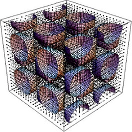
Figure 8: A visualization of the function $\mathfrak{J}(X,Y,Z)$ for the $2$-brane invariant with respect to discrete group $\mathrm{GF_{192}}$ and assigned to the representation $\mathrm{D_{7}}$ is provided by plotting equal level surfaces of the function, namely the two dimensional surfaces defined by $\mathfrak{J}(X,Y,Z)\,=\,\ell$. In the same box we plot also the gradient field $\nabla\mathfrak{J}(X,Y,Z)$, namely the vector field orthogonal to the level surfaces. The two information combined provide a sort of visualizations of the function.

We do not dwell on the fourth example of section 4.4 since the feature $\mathfrak{J}^{\mathrm{D_{9}}(\mathrm{GF_{192})}}_{\mathbf{1,1,0}}(X,Y,Z)\,=\,0$ yields a $2$-brane solution with exactly the same structure (apart from numerical factors) as the $2$-brane solution of section 5.2.2.

6 Comparison with the bosonic action of Minimal $D=7$ supergravity according to the TPvN construction.

As promised above, in this appendix we make a comparison between the action (5.10) and the bosonic action of minimal $D=7$ Supergravity as it was derived in [9], which, for brevity we name TPvN. The goal is that of verifying whether the constraint (5.25) is verified by the coefficients in the TPvN action.

Since the authors of [9] use the Dutch conventions for tensor calculus with imaginary time, the comparison of the lagrangians at the level of signs is difficult, yet at the level of absolute values of the coefficients it is possible, by means of several rescalings. First we observe that the normalization of the Einstein term in eq.(2) of TPvN is the same, if we take into account the already stressed ${\textstyle\frac{1}{2}}$ difference in the definition of the Ricci tensor and scalar curvature. Secondly we note the normalization of the dilaton kinetic term in eq.(2) of TPvN, namely ${\textstyle\frac{1}{2}}$ becomes that of the action (5.10), namely ${\textstyle\frac{1}{4}}$ if we define:

$$\phi_{TPvN}\,=\,{\textstyle\frac{1}{\sqrt{2}}}\,\varphi$$ (6.1)

A check that this is the correct identification arises from inspection of the dilaton factor in front of the three-form kinetic term. Using eq.(3) of TPvN, we see that according to this construction such a factor is:

$$\exp\left[-\,{\textstyle\frac{4}{\sqrt{5}}}\,\phi_{TPvN}\right]\,=\,\exp\left[-2\,{\textstyle\frac{2}{\sqrt{5}}}\,\varphi\right]$$ (6.2)

This confirms the value $a\,=-\,2\,{\textstyle\frac{2}{\sqrt{5}}}$ leading to the miraculous value $\Delta\,=\,4$ of the dimensional reduction invariant. Secondly we consider the necessary rescalings for the $\mathbf{A}^{[3]}$ and $\mathbf{A}^{\Lambda}$ gauge fields. Taking into account the different strengths of the exterior derivatives (see unnumbered eq.s of [9] in between eq.(1) and (2)) we see that in order to match the normalizations of (5.10) we have to define:

$${A}^{TPvN}_{\lambda\mu\nu} = {\textstyle\frac{1}{4\sqrt{2}}}\,\mathbf{A}^{[3]}_{\lambda\mu\nu}\quad\Rightarrow\quad F^{TPvN}_{\lambda\mu\nu\rho}\,=\,{\textstyle\frac{1}{\sqrt{2}}}\mathbf{F}_{\lambda\mu\nu\rho}$$

$${A}^{\Lambda|TPvN}_{\mu} = \sqrt{{\textstyle\frac{\omega}{8}}}\,\mathbf{A}^{\Lambda}_{\mu}\quad\Rightarrow\quad F^{\Lambda|TPvN}_{\lambda\mu}\,=\,\sqrt{{\textstyle\frac{\omega}{2}}}\,\mathbf{F}^{\Lambda}_{\lambda\mu}$$ (6.3)

with these redefinitions we can calculate the value of $\kappa$ according to TPvN. We find:

$${\textstyle\frac{1}{48\,\sqrt{2}}}\,F^{TPvN}_{\mu\nu\rho\sigma}F^{\Lambda|TPvN}_{\kappa\lambda}A^{\Lambda|TPvN}_{\tau}\,\epsilon^{\mu\nu\rho\sigma\lambda\kappa\tau}\,=\,{\textstyle\frac{\omega}{384}}\,\mathbf{F}_{\mu\nu\rho\sigma}\mathbf{F}^{\Lambda}_{\kappa\lambda}\mathbf{A}^{\Lambda}_{\tau}\,\epsilon^{\mu\nu\rho\sigma\lambda\kappa\tau}$$ (6.4)

which implies:

$$\kappa\,=\,{\textstyle\frac{\omega}{384}}$$ (6.5)

The above values satisfies the consistency condition (5.25), when $\Delta=4$, which has already been verified above. This shows that Arnold Beltrami flux branes are solutions of minimal $D=7$ supergravity and of no other theory of the same type which is not supersymmetric.

As we stressed in previous pages the next important step is the derivation of Killing spinors and the analysis of preserved supersymmetries. We postpone this task until we have reconstructed the entire theory within the rheonomy framework [24].

7 Conclusions

The motivations of this Sentimental Journey from Hydrodynamics to Supergravity have been extensively discussed in the introduction and will not be repeated here. The hidden link between Beltrami equation and supersymmetry was not suspected: now it has become a matter of fact. The main exciting consequence of this unveiling, already outlined in our introduction, is the injection of a vast variety of discrete symmetries into the brane-world. Such a richness of symmetries and the link with supersymmetry have to be exploited. We plane to exploit them as soon as the parallel work on $D=7$ supergravity will be finished. For the moment we can just compile a list of tasks to be accomplished which constitute our agenda for the nearest future:

1. Study of the Killing spinor equation and derivation of the supersymmetries preserved by each Arnold–Beltrami flux–brane.

2. Study the field content of the world-volume gauge theory $\mathcal{GT}_{3}$ associated with each brane. Describe the transmission of the discrete symmetries to $\mathcal{GT}_{3}$.

3. Study the topological twist of $\mathcal{GT}_{3}$ and possibly calculate its partition function[32].

4. Construct the $\kappa$-supersymmetric world-volume action of these branes.

5. Explore aspects of the Gauge/Gravity correspondence in this new setup.

The Sentimental Journey has just started and we hope it can continue and contribute to new understanding.

Aknowledgements

During the completion of this work we had a few very important and clarifying discussions with our colleagues and friends, L. Andrianopoli, L. Castellani, R. D’Auria, S. Ferrara, P.A. Grassi, A. Sagnotti and M. Trigiante. We thank them warmheartedly. The work of A.S. was partially supported by the RFBR Grants No. 16-52-12012 -NNIO-a, No. 15-52-05022-Arm-a and by the DFG Grant LE 838/12-2.

Appendix A The Group $\mathrm{GF_{192}}$ and its subgroup $\mathrm{GS_{24}}$

In this section we list all the elements of the space group $\mathrm{GF_{192}}$, organized into their $20$ conjugacy classes and of its subgroup $\mathrm{GS_{24}}$ which is isomorphic to the octahedral group $\mathrm{O_{24}}$.

A.1 $\mathrm{GF_{192}}$

Conjugacy class $\mathcal{C}_{1}\left(\mathrm{GF_{192}}\right)$: $\#$ of elements = $1$

$$\begin{array}[]{l}\left\{1_{1},0,0,0\right\}\end{array}$$ (A.1)

Conjugacy class $\mathcal{C}_{2}\left(\mathrm{GF_{192}}\right)$: $\#$ of elements = $1$

$$\begin{array}[]{l}\left\{1_{1},1,1,1\right\}\end{array}$$ (A.2)

Conjugacy class $\mathcal{C}_{3}\left(\mathrm{GF_{192}}\right)$: $\#$ of elements = $3$

$$\begin{array}[]{lll}\left\{1_{1},0,0,1\right\}&\left\{1_{1},0,1,0\right\}&\left\{1_{1},1,0,0\right\}\end{array}$$ (A.3)

Conjugacy class $\mathcal{C}_{4}\left(\mathrm{GF_{192}}\right)$: $\#$ of elements = $3$

$$\begin{array}[]{lll}\left\{1_{1},0,1,1\right\}&\left\{1_{1},1,0,1\right\}&\left\{1_{1},1,1,0\right\}\end{array}$$ (A.4)

Conjugacy class $\mathcal{C}_{5}\left(\mathrm{GF_{192}}\right)$: $\#$ of elements = $3$

$$\begin{array}[]{lll}\left\{3_{1},0,0,1\right\}&\left\{3_{2},1,1,0\right\}&\left\{3_{3},1,1,1\right\}\end{array}$$ (A.5)

Conjugacy class $\mathcal{C}_{6}\left(\mathrm{GF_{192}}\right)$: $\#$ of elements = $3$

$$\begin{array}[]{lll}\left\{3_{1},0,0,0\right\}&\left\{3_{2},1,0,0\right\}&\left\{3_{3},0,1,1\right\}\end{array}$$ (A.6)

Conjugacy class $\mathcal{C}_{7}\left(\mathrm{GF_{192}}\right)$: $\#$ of elements = $3$

$$\begin{array}[]{lll}\left\{3_{1},1,1,1\right\}&\left\{3_{2},0,1,1\right\}&\left\{3_{3},1,0,0\right\}\end{array}$$ (A.7)

Conjugacy class $\mathcal{C}_{8}\left(\mathrm{GF_{192}}\right)$: $\#$ of elements = $3$

$$\begin{array}[]{lll}\left\{3_{1},1,1,0\right\}&\left\{3_{2},0,0,1\right\}&\left\{3_{3},0,0,0\right\}\end{array}$$ (A.8)

Conjugacy class $\mathcal{C}_{9}\left(\mathrm{GF_{192}}\right)$: $\#$ of elements = $6$

$$\begin{array}[]{lll}\left\{3_{1},0,1,1\right\}&\left\{3_{1},1,0,1\right\}&\left\{3_{2},0,1,0\right\}\\ \left\{3_{2},1,1,1\right\}&\left\{3_{3},1,0,1\right\}&\left\{3_{3},1,1,0\right\}\end{array}$$ (A.9)

Conjugacy class $\mathcal{C}_{10}\left(\mathrm{GF_{192}}\right)$: $\#$ of elements = $6$

$$\begin{array}[]{lll}\left\{3_{1},0,1,0\right\}&\left\{3_{1},1,0,0\right\}&\left\{3_{2},0,0,0\right\}\\ \left\{3_{2},1,0,1\right\}&\left\{3_{3},0,0,1\right\}&\left\{3_{3},0,1,0\right\}\end{array}$$ (A.10)

Conjugacy class $\mathcal{C}_{11}\left(\mathrm{GF_{192}}\right)$: $\#$ of elements = $12$

$$\begin{array}[]{llll}\left\{4_{1},\frac{1}{2},0,0\right\}&\left\{4_{1},\frac{1}{2},1,1\right\}&\left\{4_{2},\frac{3}{2},0,0\right\}&\left\{4_{2},\frac{3}{2},1,1\right\}\\ \left\{4_{3},0,0,\frac{1}{2}\right\}&\left\{4_{3},1,1,\frac{1}{2}\right\}&\left\{4_{4},\frac{1}{2},\frac{3}{2},\frac{1}{2}\right\}&\left\{4_{4},\frac{3}{2},\frac{3}{2},\frac{3}{2}\right\}\\ \left\{4_{5},\frac{1}{2},\frac{1}{2},\frac{3}{2}\right\}&\left\{4_{5},\frac{3}{2},\frac{1}{2},\frac{1}{2}\right\}&\left\{4_{6},0,0,\frac{3}{2}\right\}&\left\{4_{6},1,1,\frac{3}{2}\right\}\end{array}$$ (A.11)

Conjugacy class $\mathcal{C}_{12}\left(\mathrm{GF_{192}}\right)$: $\#$ of elements = $12$

$$\begin{array}[]{llll}\left\{4_{1},\frac{1}{2},0,1\right\}&\left\{4_{1},\frac{1}{2},1,0\right\}&\left\{4_{2},\frac{3}{2},0,1\right\}&\left\{4_{2},\frac{3}{2},1,0\right\}\\ \left\{4_{3},0,1,\frac{1}{2}\right\}&\left\{4_{3},1,0,\frac{1}{2}\right\}&\left\{4_{4},\frac{1}{2},\frac{3}{2},\frac{3}{2}\right\}&\left\{4_{4},\frac{3}{2},\frac{3}{2},\frac{1}{2}\right\}\\ \left\{4_{5},\frac{1}{2},\frac{1}{2},\frac{1}{2}\right\}&\left\{4_{5},\frac{3}{2},\frac{1}{2},\frac{3}{2}\right\}&\left\{4_{6},0,1,\frac{3}{2}\right\}&\left\{4_{6},1,0,\frac{3}{2}\right\}\end{array}$$ (A.12)

Conjugacy class $\mathcal{C}_{13}\left(\mathrm{GF_{192}}\right)$: $\#$ of elements = $12$

$$\begin{array}[]{llll}\left\{4_{1},\frac{3}{2},0,0\right\}&\left\{4_{1},\frac{3}{2},1,1\right\}&\left\{4_{2},\frac{1}{2},0,0\right\}&\left\{4_{2},\frac{1}{2},1,1\right\}\\ \left\{4_{3},0,0,\frac{3}{2}\right\}&\left\{4_{3},1,1,\frac{3}{2}\right\}&\left\{4_{4},\frac{1}{2},\frac{1}{2},\frac{1}{2}\right\}&\left\{4_{4},\frac{3}{2},\frac{1}{2},\frac{3}{2}\right\}\\ \left\{4_{5},\frac{1}{2},\frac{3}{2},\frac{3}{2}\right\}&\left\{4_{5},\frac{3}{2},\frac{3}{2},\frac{1}{2}\right\}&\left\{4_{6},0,0,\frac{1}{2}\right\}&\left\{4_{6},1,1,\frac{1}{2}\right\}\end{array}$$ (A.13)

Conjugacy class $\mathcal{C}_{14}\left(\mathrm{GF_{192}}\right)$: $\#$ of elements = $12$

$$\begin{array}[]{llll}\left\{4_{1},\frac{3}{2},0,1\right\}&\left\{4_{1},\frac{3}{2},1,0\right\}&\left\{4_{2},\frac{1}{2},0,1\right\}&\left\{4_{2},\frac{1}{2},1,0\right\}\\ \left\{4_{3},0,1,\frac{3}{2}\right\}&\left\{4_{3},1,0,\frac{3}{2}\right\}&\left\{4_{4},\frac{1}{2},\frac{1}{2},\frac{3}{2}\right\}&\left\{4_{4},\frac{3}{2},\frac{1}{2},\frac{1}{2}\right\}\\ \left\{4_{5},\frac{1}{2},\frac{3}{2},\frac{1}{2}\right\}&\left\{4_{5},\frac{3}{2},\frac{3}{2},\frac{3}{2}\right\}&\left\{4_{6},0,1,\frac{1}{2}\right\}&\left\{4_{6},1,0,\frac{1}{2}\right\}\end{array}$$ (A.14)

Conjugacy class $\mathcal{C}_{15}\left(\mathrm{GF_{192}}\right)$: $\#$ of elements = $12$

$$\begin{array}[]{llll}\left\{5_{1},0,0,\frac{1}{2}\right\}&\left\{5_{1},1,1,\frac{1}{2}\right\}&\left\{5_{2},\frac{1}{2},\frac{3}{2},\frac{3}{2}\right\}&\left\{5_{2},\frac{3}{2},\frac{3}{2},\frac{1}{2}\right\}\\ \left\{5_{3},\frac{1}{2},\frac{1}{2},\frac{1}{2}\right\}&\left\{5_{3},\frac{3}{2},\frac{1}{2},\frac{3}{2}\right\}&\left\{5_{4},0,0,\frac{3}{2}\right\}&\left\{5_{4},1,1,\frac{3}{2}\right\}\\ \left\{5_{5},\frac{1}{2},0,1\right\}&\left\{5_{5},\frac{1}{2},1,0\right\}&\left\{5_{6},\frac{3}{2},0,1\right\}&\left\{5_{6},\frac{3}{2},1,0\right\}\end{array}$$ (A.15)

Conjugacy class $\mathcal{C}_{16}\left(\mathrm{GF_{192}}\right)$: $\#$ of elements = $12$

$$\begin{array}[]{llll}\left\{5_{1},0,0,\frac{3}{2}\right\}&\left\{5_{1},1,1,\frac{3}{2}\right\}&\left\{5_{2},\frac{1}{2},\frac{1}{2},\frac{3}{2}\right\}&\left\{5_{2},\frac{3}{2},\frac{1}{2},\frac{1}{2}\right\}\\ \left\{5_{3},\frac{1}{2},\frac{3}{2},\frac{1}{2}\right\}&\left\{5_{3},\frac{3}{2},\frac{3}{2},\frac{3}{2}\right\}&\left\{5_{4},0,0,\frac{1}{2}\right\}&\left\{5_{4},1,1,\frac{1}{2}\right\}\\ \left\{5_{5},\frac{3}{2},0,1\right\}&\left\{5_{5},\frac{3}{2},1,0\right\}&\left\{5_{6},\frac{1}{2},0,1\right\}&\left\{5_{6},\frac{1}{2},1,0\right\}\end{array}$$ (A.16)

Conjugacy class $\mathcal{C}_{17}\left(\mathrm{GF_{192}}\right)$: $\#$ of elements = $12$

$$\begin{array}[]{llll}\left\{5_{1},0,1,\frac{1}{2}\right\}&\left\{5_{1},1,0,\frac{1}{2}\right\}&\left\{5_{2},\frac{1}{2},\frac{3}{2},\frac{1}{2}\right\}&\left\{5_{2},\frac{3}{2},\frac{3}{2},\frac{3}{2}\right\}\\ \left\{5_{3},\frac{1}{2},\frac{1}{2},\frac{3}{2}\right\}&\left\{5_{3},\frac{3}{2},\frac{1}{2},\frac{1}{2}\right\}&\left\{5_{4},0,1,\frac{3}{2}\right\}&\left\{5_{4},1,0,\frac{3}{2}\right\}\\ \left\{5_{5},\frac{1}{2},0,0\right\}&\left\{5_{5},\frac{1}{2},1,1\right\}&\left\{5_{6},\frac{3}{2},0,0\right\}&\left\{5_{6},\frac{3}{2},1,1\right\}\end{array}$$ (A.17)

Conjugacy class $\mathcal{C}_{18}\left(\mathrm{GF_{192}}\right)$: $\#$ of elements = $12$

$$\begin{array}[]{llll}\left\{5_{1},0,1,\frac{3}{2}\right\}&\left\{5_{1},1,0,\frac{3}{2}\right\}&\left\{5_{2},\frac{1}{2},\frac{1}{2},\frac{1}{2}\right\}&\left\{5_{2},\frac{3}{2},\frac{1}{2},\frac{3}{2}\right\}\\ \left\{5_{3},\frac{1}{2},\frac{3}{2},\frac{3}{2}\right\}&\left\{5_{3},\frac{3}{2},\frac{3}{2},\frac{1}{2}\right\}&\left\{5_{4},0,1,\frac{1}{2}\right\}&\left\{5_{4},1,0,\frac{1}{2}\right\}\\ \left\{5_{5},\frac{3}{2},0,0\right\}&\left\{5_{5},\frac{3}{2},1,1\right\}&\left\{5_{6},\frac{1}{2},0,0\right\}&\left\{5_{6},\frac{1}{2},1,1\right\}\end{array}$$ (A.18)

Conjugacy class $\mathcal{C}_{19}\left(\mathrm{GF_{192}}\right)$: $\#$ of elements = $32$

$$\begin{array}[]{llllllll}\left\{2_{1},\frac{1}{2},\frac{1}{2},0\right\}&\left\{2_{1},\frac{1}{2},\frac{3}{2},1\right\}&\left\{2_{1},\frac{3}{2},\frac{1}{2},1\right\}&\left\{2_{1},\frac{3}{2},\frac{3}{2},0\right\}&\left\{2_{2},\frac{1}{2},\frac{1}{2},0\right\}&\left\{2_{2},\frac{1}{2},\frac{3}{2},1\right\}&\left\{2_{2},\frac{3}{2},\frac{1}{2},1\right\}&\left\{2_{2},\frac{3}{2},\frac{3}{2},0\right\}\\ \left\{2_{3},0,\frac{1}{2},\frac{3}{2}\right\}&\left\{2_{3},0,\frac{3}{2},\frac{1}{2}\right\}&\left\{2_{3},1,\frac{1}{2},\frac{1}{2}\right\}&\left\{2_{3},1,\frac{3}{2},\frac{3}{2}\right\}&\left\{2_{4},0,\frac{1}{2},\frac{1}{2}\right\}&\left\{2_{4},0,\frac{3}{2},\frac{3}{2}\right\}&\left\{2_{4},1,\frac{1}{2},\frac{3}{2}\right\}&\left\{2_{4},1,\frac{3}{2},\frac{1}{2}\right\}\\ \left\{2_{5},0,\frac{1}{2},\frac{1}{2}\right\}&\left\{2_{5},0,\frac{3}{2},\frac{3}{2}\right\}&\left\{2_{5},1,\frac{1}{2},\frac{3}{2}\right\}&\left\{2_{5},1,\frac{3}{2},\frac{1}{2}\right\}&\left\{2_{6},0,\frac{1}{2},\frac{3}{2}\right\}&\left\{2_{6},0,\frac{3}{2},\frac{1}{2}\right\}&\left\{2_{6},1,\frac{1}{2},\frac{1}{2}\right\}&\left\{2_{6},1,\frac{3}{2},\frac{3}{2}\right\}\\ \left\{2_{7},\frac{1}{2},\frac{1}{2},1\right\}&\left\{2_{7},\frac{1}{2},\frac{3}{2},0\right\}&\left\{2_{7},\frac{3}{2},\frac{1}{2},0\right\}&\left\{2_{7},\frac{3}{2},\frac{3}{2},1\right\}&\left\{2_{8},\frac{1}{2},\frac{1}{2},1\right\}&\left\{2_{8},\frac{1}{2},\frac{3}{2},0\right\}&\left\{2_{8},\frac{3}{2},\frac{1}{2},0\right\}&\left\{2_{8},\frac{3}{2},\frac{3}{2},1\right\}\end{array}$$ (A.19)

Conjugacy class $\mathcal{C}_{20}\left(\mathrm{GF_{192}}\right)$: $\#$ of elements = $32$

$$\begin{array}[]{llllllll}\left\{2_{1},\frac{1}{2},\frac{1}{2},1\right\}&\left\{2_{1},\frac{1}{2},\frac{3}{2},0\right\}&\left\{2_{1},\frac{3}{2},\frac{1}{2},0\right\}&\left\{2_{1},\frac{3}{2},\frac{3}{2},1\right\}&\left\{2_{2},\frac{1}{2},\frac{1}{2},1\right\}&\left\{2_{2},\frac{1}{2},\frac{3}{2},0\right\}&\left\{2_{2},\frac{3}{2},\frac{1}{2},0\right\}&\left\{2_{2},\frac{3}{2},\frac{3}{2},1\right\}\\ \left\{2_{3},0,\frac{1}{2},\frac{1}{2}\right\}&\left\{2_{3},0,\frac{3}{2},\frac{3}{2}\right\}&\left\{2_{3},1,\frac{1}{2},\frac{3}{2}\right\}&\left\{2_{3},1,\frac{3}{2},\frac{1}{2}\right\}&\left\{2_{4},0,\frac{1}{2},\frac{3}{2}\right\}&\left\{2_{4},0,\frac{3}{2},\frac{1}{2}\right\}&\left\{2_{4},1,\frac{1}{2},\frac{1}{2}\right\}&\left\{2_{4},1,\frac{3}{2},\frac{3}{2}\right\}\\ \left\{2_{5},0,\frac{1}{2},\frac{3}{2}\right\}&\left\{2_{5},0,\frac{3}{2},\frac{1}{2}\right\}&\left\{2_{5},1,\frac{1}{2},\frac{1}{2}\right\}&\left\{2_{5},1,\frac{3}{2},\frac{3}{2}\right\}&\left\{2_{6},0,\frac{1}{2},\frac{1}{2}\right\}&\left\{2_{6},0,\frac{3}{2},\frac{3}{2}\right\}&\left\{2_{6},1,\frac{1}{2},\frac{3}{2}\right\}&\left\{2_{6},1,\frac{3}{2},\frac{1}{2}\right\}\\ \left\{2_{7},\frac{1}{2},\frac{1}{2},0\right\}&\left\{2_{7},\frac{1}{2},\frac{3}{2},1\right\}&\left\{2_{7},\frac{3}{2},\frac{1}{2},1\right\}&\left\{2_{7},\frac{3}{2},\frac{3}{2},0\right\}&\left\{2_{8},\frac{1}{2},\frac{1}{2},0\right\}&\left\{2_{8},\frac{1}{2},\frac{3}{2},1\right\}&\left\{2_{8},\frac{3}{2},\frac{1}{2},1\right\}&\left\{2_{8},\frac{3}{2},\frac{3}{2},0\right\}\end{array}$$ (A.20)

A.2 The Group $\mathrm{GS_{24}}$

In this section we list all the elements of the space group $\mathrm{GS_{24}}$, organized into their $5$ conjugacy classes that, in this case are arranged according to the order which is customary in crystallography for the proper octahedral group.

Conjugacy class $\mathcal{C}_{1}\left(\mathrm{GS_{24}}\right)$: $\#$ of elements = $1$

$$\begin{array}[]{l}\left\{1_{1},0,0,0\right\}\end{array}$$ (A.21)

Conjugacy class $\mathcal{C}_{2}\left(\mathrm{GS_{24}}\right)$: $\#$ of elements = $8$

$$\begin{array}[]{llll}\left\{2_{1},\frac{3}{2},\frac{1}{2},1\right\}&\left\{2_{2},\frac{1}{2},\frac{3}{2},1\right\}&\left\{2_{3},1,\frac{1}{2},\frac{1}{2}\right\}&\left\{2_{4},0,\frac{3}{2},\frac{3}{2}\right\}\\ \left\{2_{5},1,\frac{3}{2},\frac{1}{2}\right\}&\left\{2_{6},0,\frac{1}{2},\frac{3}{2}\right\}&\left\{2_{7},\frac{1}{2},\frac{3}{2},0\right\}&\left\{2_{8},\frac{3}{2},\frac{1}{2},0\right\}\end{array}$$ (A.22)

Conjugacy class $\mathcal{C}_{3}\left(\mathrm{GS_{24}}\right)$: $\#$ of elements = $3$

$$\begin{array}[]{lll}\left\{3_{1},1,1,1\right\}&\left\{3_{2},0,1,1\right\}&\left\{3_{3},1,0,0\right\}\end{array}$$ (A.23)

Conjugacy class $\mathcal{C}_{4}\left(\mathrm{GS_{24}}\right)$: $\#$ of elements = $6$

$$\begin{array}[]{lll}\left\{4_{1},\frac{1}{2},1,1\right\}&\left\{4_{2},\frac{3}{2},1,1\right\}&\left\{4_{3},1,1,\frac{1}{2}\right\}\\ \left\{4_{4},\frac{1}{2},\frac{3}{2},\frac{1}{2}\right\}&\left\{4_{5},\frac{3}{2},\frac{1}{2},\frac{1}{2}\right\}&\left\{4_{6},0,0,\frac{3}{2}\right\}\end{array}$$ (A.24)

Conjugacy class $\mathcal{C}_{5}\left(\mathrm{GS_{24}}\right)$: $\#$ of elements = $6$

$$\begin{array}[]{lll}\left\{5_{1},0,1,\frac{3}{2}\right\}&\left\{5_{2},\frac{3}{2},\frac{1}{2},\frac{3}{2}\right\}&\left\{5_{3},\frac{1}{2},\frac{3}{2},\frac{3}{2}\right\}\\ \left\{5_{4},1,0,\frac{1}{2}\right\}&\left\{5_{5},\frac{3}{2},0,0\right\}&\left\{5_{6},\frac{1}{2},0,0\right\}\end{array}$$ (A.25)

References

- [1] E. Beltrami, Opere matematiche, 4 (1889) 304.
- [2] P. Fré and A.S. Sorin Classification of Arnold Beltrami Flows and their Hidden Symmetries arXiv:1501.04604 [math-ph], Physics of Elementary Particles and Atomic Nuclei, V. 46, 4 (2015).
- [3] V. I. Arnold, On the evolution of a magnetic feld under the action of transport and diffusion, in VLADIMIR I. ARNOLD: Collected Works, VOLUME II, Hydrodynamics, Bifurcation Theory, and Algebraic Geometry 1965-1972 (Edited by Alexander B. Givental, Boris A. Khesin, Alexander N. Varchenko, Victor A. Vassiliev, Oleg Ya. Viro), 405 - 419, Springer-Verlag Berlin Heidelberg 2014. Originally published in: Some Problems in Modern Analysis, 8-21 (Russian), Izd. MGU, Moscow 1984.
- [4] L.J. Romans, The F(4) supergravity in six dimensions, Nucl. Phys. B269 (1986) 691.
- [5] L. Andrianopoli, R. D’Auria and S. Vaula, Matter coupled F(4) gauged supergravity Lagrangian, JHEP 0105, 065 (2001) [hep-th/0104155].
- [6] R. D’Auria and S. Vaula, D=6, N=2, F(4) supergravity with supersymmetric de Sitter background, JHEP 0209, 057 (2002) [hep-th/0203074].
- [7] R. D’Auria, S. Ferrara and S. Vaula, AdS(6) / CFT(5) correspondence for F(4) supergravity, Fortsch. Phys. 49, 459 (2001) [hep-th/0101066].
- [8] R. D’Auria, S. Ferrara and S. Vaula, Matter coupled F(4) supergravity and the AdS(6) / CFT(5) correspondence, JHEP 0010, 013 (2000) [hep-th/0006107].
- [9] P.K. Townsend and P. van Nieuwenhuizen, Gauged Seven Dimensional Supergravity, Phys. Lett. B125 (1983) 41.
- [10] A. Salam and E. Sezgin, SO(4) Gauging of supergravity in seven dimensions, Phys. Lett. B126 (1983) 295.
- [11] E. Bergshoeff, I.G. Koh and E. Sezgin, Yang-Mills Einstein supergravity in seven dimensions, Phys. Rev. D, 32 (1985) 1353.
- [12] E. Sezgin and A. Salam, Maximal Extended Supergravity Theory in Seven-dimensions, Phys. Lett. B 118 (1982) 359.
- [13] K. Pilch, P. van Nieuwenhuizen and P. K. Townsend, Compactification of Supergravity on S(4) (Or 11 = 7 + 4, Too), Nucl. Phys. B 242 (1984) 377.
- [14] M. Pernici, K. Pilch and P. van Nieuwenhuizen, Gauged Maximally Extended Supergravity in Seven-dimensions, Phys. Lett. B 143 (1984) 103.
- [15] M. Bertolini, G. Ferretti, P. Fré M. Trigiante, L. Campos, P. Salomonson, Supersymmetric 3–Branes on Smooth ALE Manifolds with Flux, Nucl. Phys. B617 (2001) 3-42 [hep-th/0106186].
- [16] M. Bertolini, P. Di Vecchia, M. Frau, A.Lerda, R. Marotta,I. Pesando, Fractional D-branes and their gauge duals, JHEP 0102 (2001) 014, [hep-th/0011077]; M. Bertolini, P. Di Vecchia, M. Frau, A. Lerda and R. Marotta, N=2 Gauge theories on systems of fractional D3/D7 branes, Nucl. Phys. B 621, 157 (2002), [hep-th/0107057]; P. Di Vecchia, A. Lerda and P. Merlatti, N = 1 and N = 2 super Yang-Mills theories from wrapped branes, [hep-th/0205204].
- [17] M. Billó, L. Gallot and A. Liccardo, Classical geometry and gauge duals for fractional branes on ALE orbifolds, Nucl. Phys. B 614 (2001) 254 [hep-th/0105258].
-
[18]
G. James and M. Liebeck, Representations and Characters of Groups, Cambridge Mathematical
TextBooks, Cambrige University Press (1993).
M. Hamermesh, Group Theory and its applications to Physical Problems, Addison and Wesley Pub. Co. 1964. - [19] The ABC flows have been discovered by Gromeka in 1881, rediscovered by Beltrami [1], and proposed for study in the present context in [3] and [20].
- [20] S. Childress, Construction of steady-state hydromagnetic dynamos. I. Spatially periodic fields, Report MF-53, Courant Inst. of Math. Sci. (1967); New solutions of the kinematic dynamo problem, J. Math. Phys. 11 (1970) 3063 - 3076.
- [21] E.S. Fyodorov, The Symmetry of Regular Systems of Figures, (1891) Proceedings of the Imperial St. Petersburg Mineralogical Society, series 2, vol 28, pag 1-146.
- [22] M. I. Aroyo, Representations of Crystallographic Groups, preprint (2010).
- [23] B. Souvignier, Group theory applied to crystallography, preprint (2008).
- [24] L. Andrianopoli R. D’Auria, P. Fré and M. Trigiante, D=7 Minimal Supergravity Revisited, work in progress.
- [25] L. Castellani, R. D’Auria, P. Fré, Supergravity and String Theory: a geometric perspective, World Scientific, book in three volumes (1990).
- [26] P. G. Fré, Gravity: a Geometrical Course, Volume One and Volume Two, Springer 2013.
- [27] The literature on this topic is quite extended. As a general review, see the lecture notes: K. Stelle, Lectures on Supergravity p–Branes, Lectures presented at the 1996 ICTP Summer School, Trieste, hep-th/9701088.
- [28] For a comprehensive summary on M–brane solutions see also P. K. Townsend, M–Theory from its Superalgebra, Talk given at the NATO Advanced Study Institute on Strings, Branes and Dualities, Cargese, France, 26 May - 14 June 1997, [hep-th/9712004].
- [29] L. Castellani, A. Ceresole, R. D’Auria, S. Ferrara, P. Fré and M. Trigiante, M-branes and geometries, Nucl. Phys. B527 (1998) 142, [hep-th/9803039].
- [30] F. Cordaro, P. Fre, L. Gualtieri, P. Termonia and M. Trigiante, N=8 gaugings revisited: An Exhaustive classification, Nucl. Phys. B 532 (1998) 245, [hep-th/9804056].
- [31] B. de Wit, H. Samtleben and M. Trigiante, On Lagrangians and gaugings of maximal supergravities Nucl. Phys. B 655 (2003) 93, [hep-th/0212239].
- [32] P.Fré, P.A. Grassi and A.S. Sorin, Topologically Field Theories and Arnold Beltrami Flows, work in Progress.