Dead Reckoning Localization Technique for Mobile Wireless Sensor Networks

Abstract

Localization in wireless sensor networks (WSNs) not only provides a node with its geographical location but also a basic requirement for other applications such as geographical routing. Although a rich literature is available for localization in static WSN, not enough work is done for mobile WSNs, owing to the complexity due to node mobility. Most of the existing techniques for localization in mobile WSNs uses Monte-Carlo localization (MCL), which is not only time-consuming but also memory intensive. They, consider either the unknown nodes or anchor nodes to be static. In this paper, we propose a technique called Dead Reckoning Localization for mobile WSNs (DRLMSN). In the proposed technique all nodes (unknown nodes as well as anchor nodes) are mobile. Localization in DRLMSN is done at discrete time intervals called checkpoints. Unknown nodes are localized for the first time using three anchor nodes. For their subsequent localizations, only two anchor nodes are used. The proposed technique estimates two possible locations of a node Using Bézout's theorem. A dead reckoning approach is used to select one of the two estimated locations. We have evaluated DRLMSN through simulation using Castalia simulator, and is compared with a similar technique called RSS-MCL proposed by Wang and Zhu [1].

I Introduction

Localization is the process of providing each node with its geographical location. It is an important research issue in wireless sensor networks. This is because, each sensor node stamps the sensed data with its geographical location prior to transmission. The sink, distinguishes the received data based on the spatio-temporal characteristics, in which the location information is important and has a unique characteristic. Therefore, the transmitting node must be aware of its geographical position.

Localization not only provides the geographical position of a sensor node but also fills the pre-requisites for geographical routing, load balancing, spatial querying, data dissemination, rescue operations, and target tracking etc [2, 3, 4, 5, 6]. Location based routing can save significant amount of energy by eliminating the need for route discovery [7]. It can also improve the caching behaviour of applications where the requests are location dependent.

Mobility of sensor nodes increases the applicability of wireless sensor networks (WSNs). The mobility of a sensor node with respect to environment can be of two types: (i) static, and (ii) dynamic. In static, a sensor node is only data driven, i.e., to sense the environment and report to the base station (BS), while in dynamic a sensor node is not only data driven, but also serves as an actuator. In both the cases, position of nodes changes oftenly. As a result, a node in mobile WSNs is localized more than once, compared to static WSNs - where a node is localized only once at the initialization of network. The continuous localization of nodes with mobility results in: (i) faster battery deletion and hence, reduces the lifetime of sensor nodes, and (ii) increases the communication cost. On the contrary, mobility improves: (i) coverage of WSN - uncovered locations at one instant can be covered at some other instant of time, (ii) enhances the security - intruders can be detected easily as compared to the static WSNs, and (iii) increases connectivity - mobility increases the neighbours of a node [8].

The geographical position of a sensor node is determined either with the help of global positioning system (GPS) equipment or estimated from the location of neighbouring nodes. A network with all GPS enabled nodes is not a universal solution. This is because besides increasing the cost, size, and power consumption; it fails to localize in indoors, and dense forests. An alternative solution is to equip only a minimal number of nodes called anchor nodes/seeds with GPS, and the remaining nodes estimate their location using the location information of anchor nodes. A mobile WSN can be in one of the following scenarios [7, 9, 10, 11, 12, 13, 14, 15, 16, 17, 18, 19, 20, 21]:

1. Normal nodes are static, and seeds are moving: In this scenario, mobile anchor nodes ($\geq 1$) continuously broadcast their location. As soon as a static node receives three or more beacons, it localizes itself. Accuracy and localization time depends mostly on the trajectory followed by the seeds.

2. Normal nodes are moving, and seeds are static: In this scenario, each normal node is expected to receive the beacons at the same instant of time. Otherwise, it results into inaccurate estimated location. With time span the previous estimated location becomes obsolete. As a result, nodes localize repeatedly at fixed intervals with newly received seed locations. One of the appropriate example for this scenario is battlefield, where normal nodes are attached to military personnel and seeds are fixed a priori as landmarks within the battlefield. This not only helps in detecting the current position but also in providing feedback from a particular area of battlefield.

3. Both the normal nodes, and seeds are moving: This scenario is the most versatile, and complex among all the three. In this, the topology of the network changes very often. It is difficult for a normal node to get fine grained location. Therefore, the localization error is comparatively higher than the previous two scenarios.

In this paper, we propose a localization technique for the scenario, where both the normal nodes and seeds are moving. We have considered this scenario because: (i) a little emphasis is given, owing to its complexity, and (ii) to the best of our knowledge whatever little localization techniques exist for this scenario are range free based. The proposed technique is called Dead Reckoning Localization Technique (DRLMSN). Due to node mobility the position of nodes changes frequently. Localizing the nodes at every instant will drain their battery power at a faster rate. Therefore, in DRLMSN nodes are localized at discrete time intervals called checkpoints. Nodes are localized for the first time using trilateration mechanism. In their subsequent localizations, only two anchor nodes are used. Bézout's theorem [22] is used to estimate the positions of a node, and a dead reckoning technique is used to select the correct position. DRLMSN is compared with RSS-MCL [1].

The rest of the paper is organized as follows: Section II provides an overview of various localization techniques. Proposed localization algorithm is described in Section III. Simulation and results are presented in Section IV, and conclusions are drawn in Section V.

II Related work

Localization algorithms for WSNs can be broadly categorized into two types: Range based, and Range free. Range based localization algorithms uses range (distance or angle) information from the beacon node to estimate a sensor node's location [23]. They need at least three beacon nodes to estimate the position of a node. Several ranging techniques exist to estimate the distance of a node to three or more beacon nodes. Based on this information, location of a node is determined. A few representative of range based localization algorithms include: Received signal strength indicator (RSSI) [24], Angle-of-arrival (AoA) [25], Time-of-arrival (ToA) [26], Time difference of arrival (TDoA) [25]. These schemes often need extra hardware such as antennas and speakers, and their accuracy is affected by multi-path fading and shadowing.

Range-free localization algorithms use only connectivity information between unknown node and landmarks - which obtain their location information using GPS or through an artificially deployed information. Some of the range-free localization algorithms include: Centroid [27], Appropriate point in triangle (APIT) [28], and DV-HOP [29]. Centroid counts the number of beacon signals it has received from the pre-positioned beacon nodes and achieves localization by obtaining the centroid of received beacon generators. DV-HOP uses location of beacon nodes, beacon hop count, and the average distance per hop for localization. APIT algorithm requires a relatively higher ratio of beacons to nodes and longer range beacons for localization. They are susceptible to erroneous reading of RSSI. He et al. [30] showed that APIT algorithm requires lesser computation than other beacon based algorithms and performs well when the ratio of beacon to node is higher. A brief review of different localization algorithms proposed in the literature for mobile sensor networks is presented below:

In [31], authors proposed two classes of localization approaches for mobile WSNs. They are: (i) Adaptive, and (ii) Predictive. Adaptive localizations dynamically adjust their localization period based on the recent observed motion of the sensor, obtained from examining the previous locations. This approach allows the sensors to reduce their localization frequency when the sensor is slow, or increase when it is fast. In the predictive approach, sensors estimate their motion pattern and project their future motion. If the prediction is accurate, which occurs when nodes are moving predictably, location estimation may be generated. However, their main focus was on how often the localization should be done, and not on the localization process itself.

Bergamo and Mazzimi [13] proposed a range based algorithm for localizing mobile WSNs. They used fixed beacons placed at two corners on the same side of a rectangular space. Mobile sensor uses beacon signals to compute their relative position. Sensors estimate their power level from the received beacon and compute their position by triangulation method. They also studied the effect of mobility and fading on location accuracy. Placing beacons at fixed position limits the localization area. This is because the quality of RSSI decreases with distance due to various factors. This results in inaccurate distance measurement.

Hu and Evans [7] proposed a range free technique based on Monte-Carlo Localization (MCL). This technique is used for localization of robots in a predefined map. It works in two steps: First, the possible locations of an unknown node is represented as a set of weighted samples. In the next stage, invalid samples are filtered out by incorporating the newly observed samples of seed nodes. Once enough samples are obtained, an unknown node estimate its position by taking the weighted average of the samples. In this technique, the sample generation is computationally intensive and iterative in nature. This also needs a higher seed density.

Aline et al. [32] proposed a scheme to reduce the sample space generated in [7]. They named it as Monte-Carlo Boxed (MCB) scheme. Sample generation is restricted within the bounding box, which is built using 1-hop and 2-hop neighbouring anchor nodes. The neighbouring anchor information is also used in the filtering phase. The number of iterations to construct the sample space is reduced. However, the localization error in MCB is not reduced, if the number of valid samples is same as that in MCL.

Using MCL technique, Rudafshani and Datta [33] proposed two algorithms called MSL and MSL*. Static sensor nodes are localized in MSL* too. It uses sample set of all 1-hop and 2-hop neighbour of normal nodes, and anchor nodes. This resulted in better position estimation with increased memory requirement and communication cost. In MSL, a node weight its samples using the estimated position of common neighbour nodes. MSL* outperforms MSL in most scenarios, but incurs higher communication cost. MSL outperforms MSL* when there is significant irregularity in the radio range. Accuracy of common neighbouring nodes are determined by their closeness value. Closeness value of a node P with N samples is computed as:

${Closeness_{P}}=\dfrac{\sum_{i=1}^{N}W_{i}\sqrt{(x_{i}-x)^{2}+(y_{i}-y)^{2}}}{N}$

where ($x,y$) is P's estimated position and ($x_{i},y_{i}$) is P's $i^{th}$ sample with weight $W_{i}$. Both MSL and MSL* needs higher anchor density and node density. Also, when maximum velocity is large, performance of both MSL and MSL* reduces to a greater extent. Furthermore, the size of bounding box for sample generation is reduced in [34], using the negative constraint of 2-hop neighbouring anchor nodes. This reduces the computational cost for obtaining samples, and a higher location accuracy is achieved under higher density of common nodes.

Wang and Zhu et al. [1] proposed the RSS based MCL scheme which sequentially estimates the location of mobile nodes. First, it uses a set of samples with related weights to represent the posterior distribution of node's location. Next, it estimate the node's location recursively from the RSS measurement within a discrete state-space localization system. Accuracy of this scheme depends on the number of samples used and the log normal statistical model of RSS measurements. It improves the localization accuracy using both the RSSI and MCL techniques. However, it is time intensive to the sampling procedure. Also, the frequent sampling at regular intervals consume more energy of the nodes.

Comparison of different localization techniques is shown in Table I.

Localization Technique	Type	Mechanism	Mobility Model	Comments
Tilak et al. [31]	Range Free	Triangulation	Random Waypoint Model (RWP), Gaussian Markovian Model	Emphasized on localization frequency rather than localization accuracy.
Bergamo and Mazzimi [13]	Range Based	Triangulation	RWP	Limits the localization area, consider static beacon nodes.
Hu and Evans [7]	Range Free	Sequential MCL	RWP, Reference Point Group Model [35]	Slow in convergence, slower sampling technique.
Baggio and Langendoen [32]	Range Free	MCL Boxed	Modified RWP with pause time = 0 & minimum node speed = 0.1 m/s.	Lesser the sample space, more the localization error.
Rudafshani and Datta [33]	Range Free	Particle filtering approach of MCL	Modified RWP with pause time = 0 second.	Computationally intensive, higher communication cost, requires higher anchor & node density
Wang and Zhu [1]	Range Based	Sequential MCL	RWP	Accuracy depends on the sampling quality, and the RSSI model.

TABLE I: Comparison of different localization techniques for Mobile WSN.

III Dead Reckoning Localization Technique

In this section, we propose a range based, distributed localization algorithm for mobile WSNs. The proposed technique is called Dead Reckoning Localization Technique (DRLMSN). Nodes in DRLMSN are classified into the following three types: (i) Anchor node ($\mathcal{A}$): A node which can locate its own position, and is usually equipped with GPS, (ii) Normal/unknown node ($\mathcal{U}$): Nodes which are unaware of their location, and uses localization algorithm to determine their position, and (iii) Settled node ($\mathcal{S}$): These are normal nodes that have obtained their location information through a localization technique. They serve as an anchor node for the remaining unknown nodes.

To localize normal mobile nodes accurately with the help of mobile anchor nodes is a difficult task. This is because the transmitter as well as the receiver changes their position at every time instant. Therefore, to localize, a normal node must receive beacons from all the neighbouring nodes at the same time instant. Beacon are frequently advertised from the anchor/settled nodes. This advertisement contains the anchor/settled node's identiy, and location. Continuous localization of mobile nodes will drains their battery power at a faster rate. As a result, the lifetime of sensor nodes as well as the sensor network is reduced.

Sensor nodes in DRLMSN are localized during a time interval called checkpoint. There are two localization phases in DRLMSN. First phase is called Initialization phase. In this phase, a node is localized using trilateration mechanism. A node remains in the initialization phase until it localizes using trilateration mechanism. The subsequent localization phase is called Sequent phase. In this phase, a node localizes itself using only two anchor nodes. Bézout's theorem [22] is used to estimate locations of a node. A dead reckoning approach is used to identify their correct estimated position. Once a node is localized in either of the above two phases, it act as a settled node and broadcast beacons during the checkpoint. Initialization and Sequent phases are explained below.

III-A Initialization Phase:

At the beginning of a checkpoint, each anchor node broadcasts a beacon. A normal node localizes itself for the first time during the checkpoint using three anchor nodes. As soon as, a node localizes, it broadcasts a beacon during the same checkpoint. This results in the localization of one/two beacon deficit nodes. This process continues until the end of the checkpoint.

At the end of the checkpoint, some nodes may fail to localize. The possible reasons for localization failure and the corresponding actions to be taken are: i) A normal node receives only one (or two) beacon. In this case, normal node deletes the received beacons and moves on. In the subsequent checkpoint it attempts to localize using three beacons. ii) A normal node receives no beacon. In this case, a node moves on and attempts to localize itself in the next checkpoint using three beacons.

III-B Sequent Phase:

A node goes to the sequent phase only after itself localizes using trilateration mechanism. In this phase, each normal node localizes with only two nearest location aware nodes (anchor / settled node). A normal node that receives two beacons, can estimate its two positions using Bézout's theorem. According to Bézout's theorem ``The intersection of a variety of degree $m$ with a variety of degree $n$ in complex projective space is either a common component or it has $mn$ points when the intersection points are counted with the appropriate multiplicity''. Positions estimation of a node using Bézout's theorem is explained below.

Let $(x,y)$ be the position of an unknown node, and $(a_{1},b_{1})$, $(a_{2},b_{2})$ be the position of two of its neighbouring anchor nodes. Also, let the distance between an unknown node, and the respective anchor nodes be $d_{1}$ and $d_{2}$ respectively. Then,

$$(x-a_{1})^{2}+(y-b_{1})^{2}={d_{1}}^{2}$$ (1)

$$(x-a_{2})^{2}+(y-b_{2})^{2}={d_{2}}^{2}$$ (2)

Re-arranging (1) and (2), we obtain:

$$x^{2}+y^{2}={d_{1}}^{2}-{a_{1}}^{2}-{b_{1}}^{2}+2a_{1}x+2b_{1}y$$ (3)

$$x^{2}+y^{2}={d_{2}}^{2}-{a_{2}}^{2}-{b_{2}}^{2}+2a_{2}x+2b_{2}y$$ (4)

Comparing (3) and (4), we have

$${d_{1}}^{2}-{a_{1}}^{2}-{b_{1}}^{2}+2a_{1}x+2b_{1}y={d_{2}}^{2}-{a_{2}}^{2}-{b_{2}}^{2}+2a_{2}x+2b_{2}y$$ (5)

$$2(a_{1}-a_{2})x=({d_{2}}^{2}-{a_{2}}^{2}-{b_{2}}^{2}-{d_{1}}^{2}+{a_{1}}^{2}+{b_{1}}^{2})+2(b_{2}-b_{1})y$$ (6)

Let $z_{0}={d_{2}}^{2}-{a_{2}}^{2}-{b_{2}}^{2}-{d_{1}}^{2}+{a_{1}}^{2}+{b_{1}}^{2}$
The eqation (6) can be reduced to

$$x=\dfrac{z_{0}+2(b_{2}-b_{1})y}{2(a_{1}-a_{2})}$$ (7)

For simplification, this can be written as

$$x=z+py$$ (8)

where $z=\dfrac{z_{0}}{2(a_{1}-a_{2})}$ , and $p=\dfrac{2(b_{2}-b_{1})}{2(a_{1}-a_{2})}$
Substituting the value of $x$ in equation (1), we obtained

$$(p^{2}+1)y^{2}+(2zp-2a_{1}p-2b_{1})y-({d_{1}}^{2}-{a_{1}}^{2}-{b_{1}}^{2}-{z}^{2}+2a_{1}z)=0$$ (9)

Solving the quadratic equation (9), let the values obtained be $y_{1}$ and $y_{2}$. Let $x_{1}$ and $x_{2}$ be the values corresponding to $y_{1}$ and $y_{2}$ respectively. Therefore, the proposed algorithm estimates two positions $\mathit{P_{1}}$$(x_{1},y_{1})$, and $\mathit{P_{2}}$$(x_{2},y_{2})$.

In order to select the correct estimated position a dead reckoning approach is used. In this approach, a localized node say $\mathit{k}$ uses the location, $p_{prev}$ at the checkpoint $\mathit{t_{i}}$ to estimate its location in the next checkpoint at $\mathit{t_{i+1}}$. Let $\mathit{v}$ be the velocity and $\mathit{t}$ be the time interval between the two successive checkpoints. Distance $\mathit{d}$ traveled by the node $\mathit{k}$ between two successive checkpoints is calculated as $\mathit{d=v*t}$. Therefore, at the checkpoint $\mathit{t_{i+1}}$, an unknown node knows its position at checkpoint $\mathit{t_{i}}$ and the distance $\mathit{d}$ traveled between the two successive checkpoints. Also, the node has two anchor positions, i.e., $(a_{1},b_{1})$, $(a_{2},b_{2})$. Then, the node uses trilateration to calculate the position $\mathit{P}$$(\hat{x},\hat{y})$. Next, the node computes the correction factor $\mathit{Cf}$ to select one of the two estimated positions $\mathit{P_{1}}$ and $\mathit{P_{2}}$. The correctness factor is computed as:

$Cf_{1}=\sqrt{(\hat{x}-x_{1})^{2}+(\hat{y}-y_{1})^{2}}$

$Cf_{2}=\sqrt{(\hat{x}-x_{2})^{2}+(\hat{y}-y_{2})^{2}}$

where $Cf_{1},Cf_{2}$ represents the distance of position $\mathit{P_{1}}$, and $\mathit{P_{2}}$ from the position $\mathit{P}$ estimated via trilateration. The correct position of the node is $\mathit{P_{1}}$$(x_{1},y_{1})$ if ${Cf_{1}}<{Cf_{2}}$ else the correct position is $\mathit{P_{2}}$$(x_{2},y_{2})$. This is because, calculated position $\mathit{P}$$(\hat{x},\hat{y})$ always deviate from the actual position by a small margin. Once a node is localized, it broadcasts beacons until the end of the checkpoint.

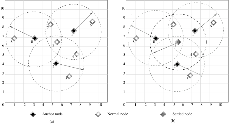
Figure 1: Initialization phase: (a) At the first checkpoint, anchor nodes transmit beacons, and normal nodes gets localized via trilateration; (b) normal nodes that are short of 1 or 2 beacons gets localized with the help of settled nodes.

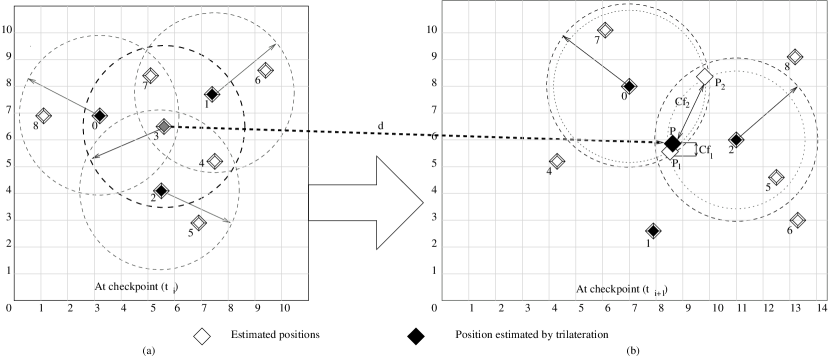
Figure 2: Normal node 3 at checkpoint $\mathit{t_{i+1}}$ estimates two locations $\mathit{P_{1}}$ and $\mathit{P_{2}}$ using two anchor nodes 0 and 2. The correct position is selected using the previous position of node 3 at checkpoint $\mathit{t_{i}}$.

We illustrate the localization process in proposed scheme using Fig. 1. Localization in the initialization phase is shown in Fig. 1(a) and 1(b). Node 3 in Fig. 1(a) receives beacon from three anchor nodes $0,1,$ and $2$ at checkpoint $t_{i}$ and gets localized. Nodes 4 and 7 receives only two beacons, whereas nodes 5, 6, and 8 receives only one beacon. These nodes at this point of checkpoint $t_{i}$ can not localize, as the number of beacons required for localization for the first time is three. Node 3 broadcast a beacon after localization. Nodes 4 and 7 gets localized after receiving beacon from node 3. This is shown in Fig. 1(b). This co-operative, distributive process of localization continues until the end of the checkpoint. At the end of the checkpoint $t_{i}$, nodes 6 and 8 have only one beacon. Both the nodes delete the received beacons and continues moving.

Fig. 2(b) illustrate the sequent phase at checkpoint $t_{i+1}$. We consider node 3, to explain localization using two anchor nodes. Let the co-ordinate of node 3 at checkpoint $t_{i}$ be $(5.5,6.3)$ as shown in Fig. 2(a), and the distance traversed during the checkpoint interval $t_{i}$ and $t_{i+1}$ be $3.5$ unit. At checkpoint $t_{i+1}$, node 3 can be localized using two anchor nodes 0 and 2, as shown in Fig. 2(b). Let the co-ordinates of node 0 and 2 be $(7,8)$ and $(11,6)$ respectively as shown in Fig. 2(b). Using Bézout's theorem node 3 estimates two locations $\mathit{P_{1}}(8.54,5.54)$ and $\mathit{P_{2}}(9.98,8.24)$. To select one of the above two locations dead reckoning approach is used. Based on the location of node 0, node 2 and its previous location, node 3 estimates its new location $\mathit{P}$$(\hat{x},\hat{y})$ equal to $(8.78,6.03)$ using trilateration technique. Then, node 3 calculates the correctness factor ${Cf_{1}}$ and ${Cf_{2}}$ to find the least deviated estimated position from $\mathit{P}$$(\hat{x},\hat{y})$. The computed value of ${Cf_{1}}$ and ${Cf_{2}}$ is 0.738 and 2.514 respectively. Since ${Cf_{1}}<{Cf_{2}}$ the position $\mathit{P_{1}}(8.54,5.54)$ is selected as the correct estimated position. It can be observed from the Fig. 2(b) the actual position of node 3 is very close to the estimated position.

The proposed localization algorithm is given as Algorithm 1.

Notation: $\mathcal{A}$: Anchor node, $\mathcal{U}$: Unknown node, $\mathcal{S}$: Settled node

Variables for $\mathcal{U}$ and $\mathcal{S}$:

1 $beaconSet\leftarrow\phi$

  /* Set of received locations (x,y). */

2 $locfirst\leftarrow 0$

  /* Set to 1, if $\mathcal{U}$ has completed initialization phase. */

3 ${P_{prev}}\leftarrow-1$

  /* Stores current estimated position of $\mathcal{S}$ used in next checkpoint. */

4 ${Status}$

  /* Indicates node type: Its value can be $\mathcal{A}$ or $\mathcal{U}$ or $\mathcal{S}$ */

/* This algorithm is distributed and event oriented in nature. So, in each node type ($\mathcal{A}$, $\mathcal{U}$, $\mathcal{S}$) different actions get fired according to event triggered (recursive time interval for checkpoint or beacon reception).*/

For Anchor Node:

5 if $Status=\mathcal{A}$ then

      6 broadcast $beacon$

      7 exit

      

For Unknown/Settled Node:

8 if $Status=\mathcal{U}$ then

      9 Repeat the steps 10 and 11 until

       (!( $(sizeof(beaconSet)\geq 3)$ AND $(locfirst=0)$) OR !($(sizeof(beaconSet)\geq 2)$ AND $(locfirst=1)$)) AND !(End of Checkpoint)

      10 received $beacon$

        /* A node monitors the beacon until the end of checkpoint or either one of the following happens: 1. Unknown node has received three beacons, 2. Settled node has received two beacons. */

      11 $beaconSet\leftarrow beaconSet\cup{\{beacon\}}$

      12 if $(sizeof(beaconSet)\geq 3)$ and $(locfirst=0)$ then /* Initialization phase. */

            13 $Position\leftarrow Trilateration(beaconSet)$

              /* Localize using Trilateration. */

            14 broadcast $beacon$

              /* Broadcast estimated position. */

            15 ${P_{prev}}\leftarrow Position$

            16 $locfirst\leftarrow 1$

            17 $Status\leftarrow\mathcal{S}$

      

      18else if $(sizeof(beaconSet)\geq 2)$ and $(locfirst=1)$ then /* Sequent phase. */

            19 $Position\leftarrow$ Use $beaconSet$ and ${P_{prev}}$

              /* Localize using dead reckoning. */

            20 broadcast $beacon$

              /* Broadcast estimated position. */

            21 ${P_{prev}}\leftarrow Position$

            22 $Status\leftarrow\mathcal{S}$

            

      

else

      23 delete $beacon$

        /* $\mathcal{A}$ or $\mathcal{S}$ do not need beacon as these are localized already */

      

/* Within different checkpoints a node remember only the values of ${P_{prev}}$ and $locfirst$.*/

24 while ((End of checkpoint) AND ($Status=\mathcal{S}$ OR $\mathcal{U}$)) do

      25 $beaconSet\leftarrow\phi$

        /* At the end of checkpoint delete received beacons. */

      26 $Status\leftarrow\mathcal{U}$

        /* For localizing in next checkpoint settled node changes status to $\mathcal{U}$. */

      

Algorithm 1 DRLMSN Localization algorithm

Description of Algorithm 1: The above algorithm is called at each node in the start of each checkpoint. In each checkpoint, anchor nodes broadcast beacons. This is mentioned in lines 5 – 7 of Algorithm 1. Line 12 – 17 localizes a node in the initialization phase. In this phase a node needs three beacons and gets localized via trilateration. Sequent phase localization is mentioned in lines 18 – 22. In this phase a node require only two beacon node for localization. This phase uses dead reckoning approach for the unambiguous localization of unknown node. Lines 6, 14, and 20 in the algorithm does the job of beacon broadcast.

IV Performance Evaluation

We have simulated the proposed scheme using Castalia simulator [36] that runs on the top of OMNET++. We have made the following assumptions in our simulation: (i) nodes are considered to be homogeneous, with respect to transceiver power and receiver sensitivity. This helps in controlling the connectivity between nodes in the network easily; (ii) for simplicity, we consider transmission range of all the nodes as a perfect circle; and (iii) all the three beacon nodes are synchronized. This results in the accurate localization of unknown nodes which otherwise tries to localize with obsolete beacons.

The key metrics used for evaluating the localization algorithm is the accuracy in location estimation. We have calculated the estimated error as the difference between the estimated position and the actual position. The average root mean square error (RMSE) is calculated as:

$Average\hskip 3.00003ptRMSE=\dfrac{\sum_{i=1}^{N-P}||\hat{\theta}_{i}-\theta_{i}||}{N-P}$

where $\hat{\theta}_{i}$ is estimated position, $\theta_{i}$ is actual position, $N$ is the total number of nodes in the network, and $P$ is number of anchor nodes.

We have considered the following parameters in our simulation: (i) nodes are randomly deployed in a sensor field of area $200\times 200$ $m^{2}$; (ii) symmetric communication within a communication range of 20 meters; (iii) anchor node density is 10%. We have defined the anchor density as the ratio between he anchor nodes to the total nodes in the network; (iv) transmission power is -5 dBm; (v) path loss exponent ($\eta$) is 2.4; and (vi) modified random waypoint mobility model [37] and random direction mobility model [38]. We have compared DBNLE with another range based localization technique called RSS-MCL proposed by Wang and Zhu [1]. Through simulation, we studied the impact of mobility model, anchor density, node speed, number of normal nodes, and deployment topology on location estimation. Each of the above parameter is explained below.

Figure 3: Impact of increase in the number of nodes on the localization error in modified random waypoint mobility model.

Figure 4: Impact of increase in the number of nodes on the localization error in random direction mobility model.

Figure 5: Mobility pattern of nodes in random waypoint mobility model.

Figure 6: Mobility pattern of nodes in random direction mobility model.

Impact of Mobility Model: Mobility pattern plays an important role in the localization process. Besides increasing the network connectivity and coverage area, mobility affects the localization accuracy, also drains the battery quickly, and the percentage of localized nodes. We considered two mobility models (i) Random Waypoint Mobility Model (RWMM), (ii) Random Direction Mobility Model (RDMM) and have shown the effect of mobility model on localization accuracy.

In RWMM, a node randomly chooses a new destination in a direction between [0, 2$\pi$] and moves towards that destination with a speed in the range [$v_{min},v_{max}$]. While in RDMM, a node randomly chooses a direction between [0, 2$\pi$], a speed in the range [$v_{min},v_{max}$] and moves in the chosen direction upto the boundary of the network. After reaching the boundary same process is repeated. In both RWMM and RDMM, a node pauses for some predefined time before changing its direction. We have set the pausetime to be zero, in order to simulate a continuous mobility model. From Fig. 4 it is observed that RWMM have lower average RMSE than RDMM as shown in Fig. 4. The reason for this difference in error is due to mobility pattern of nodes. In RWMM, nodes mostly move within the vicinity of the center. They are less likely to move towards the boundaries of the network as shown in Fig. 6. Therefore, a node will have relatively higher number of neighbours. As a result, a normal node selects the most nearest neighbours which results in lesser inaccuracy. In contrast to this, a node moves uniformly throughout the field in RDMM as shown in Fig. 6. This type of movement does not favor the selection of best neighbours, because a node is surrounded by lesser number of neighbours. It is observed from the Fig. 4 and 4 that average RMSE is lesser in DBNLE compared to RSS-MCL. This is because in RSS-MCL the number of beacons used to filter the generated sample is more compared to DBNLE which uses only 2–3 beacons. Due to mobility, increasing dependency on the number of beacons used increases the uncertainty in position estimation. Among the two mobility models, RDMM increases network coverage while RWMM increases the connectivity among nodes.

Figure 7: Impact of increase in anchors on the localization error in modified random waypoint mobility model.

Figure 8: Impact of increase in anchors on the localization error in random direction mobility model.

Impact of anchor nodes: For a fixed network size, increasing the anchor density results in the localization of more nodes in lesser time. This is because, most of the nodes obtain higher number of anchor nodes as their neighbour. To find the effect of anchor density on localization error we varied the anchor density between 5% to 20% keeping the total number of nodes to be fixed at 200. The plot for anchor density vs. localization error in RWMM and RDMM is shown in Fig. 8 and 8 respectively. It is observed from the figures that the average RMSE decreases with the increase in the anchor density. This is because: (i) higher the anchor density, lesser the number of nodes to be localized; (ii) a node gets more number of accurate beacons - resulting in lesser error accumulation and propagation. It is also observed that with an increase in anchor density the average rate of decrease of RMSE is higher, and at a higher anchor density the rate of decrease is lesser. Increase in the number of anchors do not affect average RMSE to a greater extent in RSS-MCL as compared to DBNLE. This is because in RSS-MCL position estimation depends heavily on the quality of sample generation where as in DBNLE it directly depends on the number of beacons received. Furthermore, average RMSE is lesser in RWMM as compared RWDM. This is attributed to the neighbor density. In RWMM, a node has higher neighbour density as compared to RDMM.

Impact of node speed: The effect of speed on average RMSE by varying the anchor and node density is shown in Fig. 4, 4, 8, and 8. It is observed from the above figures that with increase in speed the localization error also increases. Above figures show that the location estimation of a node in mobile WSNs is greatly affected by the node speed. A node covers more distance per unit time at higher speed. This increase in speed results in: (i) increase in the uncertainty of localizing a node accurately, as the area over which a node needs to be localized increases, (ii) with the increase in distance covered, multi-path fading and shadowing comes into play. This affects the distance measurements and decreases the efficiency of range based localization algorithm, (iii) it also affects the basic functionality, i.e., sensing is not properly done when a node moves too fast, (iv) it increases the localization percentage in low anchor density networks because increase in speed increases the network coverage.

Figure 9: Impact of node deployment on the localization error in modified random waypoint mobility model.

Figure 10: Impact of node deployment on the localization error in random direction mobility model.

Impact of normal nodes: The plot for normal nodes vs. localization error is shown in Fig. 4 and 4 respectively. With increase in the number of normal nodes there is a significant increase in the percentage of localized nodes. This also results in the decrease of localization time and localization error. Decrease in localization time is attributed to more number of localized neighbours of a normal node. It is observed from the Fig. 4 and 4 that localization error decreases gradually with the increase of nodes. The reason for this decrease is the selection of more number of nearest in-range neighbours. Closer is the neighbour lesser is the ranging error; as the quality of signal (RSSI) is directly affected by the distance between the transmitter and receiver node.

Impact of deployment/topology of nodes: Next, we consider the effect of deployment on localization error. We have considered two deployment scenarios: (i) random, and (ii) grid to study their effect on localization error. It is observed that in some cases nodes do not localize early and takes longer time to localize. Consequently, this increases the localization time of whole network. This is due to the non-availability of requisite number of beacons for localization. One of the major reason for this is the way in which nodes are deployed initially and the manner in which nodes move. It is observed that if nodes are randomly deployed, then 30% of the nodes fail to localize in the first 2 to 3 checkpoints, whereas in grid network around 90% of nodes localize in the first checkpoint itself. In the next checkpoint all nodes get localized. From the Fig. 10 and 10, it is observed that the localization error is lesser in grid deployment than in random deployment.

Figure 11: Percenatge of localized nodes at successive checkpoints in modified random waypoint mobility model.

Figure 12: Percenatge of localized nodes at successive checkpoints in random direction mobility model.

Finally, we studied the percentage of nodes localized at different checkpoints. The plot for percentage of localized nodes vs. checkpoints is shown in Fig. 12 and 12. It is observed that the percentage of nodes localized increases as the checkpoint increases. Majority of the nodes gets localized after the fourth checkpoint. Percentage of localized nodes in RSS-MCL is relatively lesser as compared in DRLMSN. This is because the time spent in sample generation and filtering is more than checkpoint duration. As a result, most of the nodes fail to localize in RSS-MCL due to this time constraint.

V Conclusion

A large number of localization techniques have been developed for static WSNs. These techniques can not be applied to mobile WSNs. Only a few localization techniques has been proposed for mobile WSNs. Most of these techniques considered either normal node or anchor nodes to be static. In this paper we propose a technique called dead reckoning localization for mobile WSN. We have considered both the normal nodes and anchor nodes to be mobile. As the nodes move in a sensor field, their position changes with time. Therefore, a mobile node has to be localized as long as it is alive. In the proposed technique, nodes are localized at discrete time intervals called checkpoints. A normal node is localized for the first time using three anchor nodes. For their subsequent localizations only two anchor nodes are used and a dead reckoning technique is applied. Reduction in the number of anchor nodes required for localization from three to two result in faster localization and lesser localization error. We have compared the proposed scheme with an existing similar scheme called RSS-MCL. It is observed that the proposed scheme has faster localization time with lesser localization error than RSS-MCL. We have also studied the impact of node density, anchor density, node speed, deployment type and mobility pattern on localization. It was observed that the above parameters have strong influence in the localization time and localization error.

In future we would like to check the validty of DRLMSN with different mobility models other than RWMM and RDMM. Also, to implement the proposed scheme in an real environment and check its performance.

References

- [1] W. D. Wang and Q. X. Zhu. RSS-Based Monte Carlo Localisation for Mobile Sensor Networks. IET Communications, 2(5):673–681, 2008.
- [2] A. Caruso, S. Chessa, S. De, and R. Urpi. GPS Free Coordinate Assignment and Routing in Wireless Sensor Networks. In IEEE INFOCOM, pages 150–160, 2005.
- [3] N. I. Dopico, B. B. Haro, S. V. Macua, P. Belanovic, and S. Zazo. Improved Animal Tracking Algorithms Using Distributed Kalman-based Filters. In European Wireless, 2011.
- [4] N. Patwari, J. N. Ash, S. Kyperountas, A. O. Hero III, R. L. Moses, and N. S. Correal. Locating the Nodes: Cooperative Localization in Wireless Sensor Networks. IEEE Signal Processing Magazine, 22(4):54–69, 2005.
- [5] R. Yu, Y. Zhang, K. Yang, S. Xie, and H.-H. Chen. Distributed Geographical Packet Forwarding in Wireless Sensor and Actuator Networks - a Stochastic Optimal Control Approach. IET Wireless Sensor Systems, 2(1):63–74, March 2012.
- [6] J. Hightower and G. Borriello. Location Systems for Ubiquitous Computing. Computer, 34(8):57–66, Aug. 2001.
- [7] L. Hu and D. Evans. Localization for Mobile Sensor Networks. In Proceedings of the 10th annual International Conference on Mobile Computing and Networking, MobiCom '04, pages 45–57, Philadelphia, PA, USA, 2004. ACM.
- [8] Y. Liu and Z. Yang. Location, Localization, and Localizability, chapter Localization for Mobile Networks, pages 97–109. Springer, ist edition, 2011.
- [9] A. Galstyan, B. Krishnamachari, K. Lerman, and S. Pattem. Distributed Online Localization in Sensor Networks Using a Moving Target. In Third International Symposium on Information Processing in Sensor Networks (IPSN), ISPN 04, pages 61–70, 26-27 April 2004.
- [10] P. N. Pathirana, N. Bulusu, A. V. Savkin, and S. Jha. Node Localization Using Mobile Robots in Delay-Tolerant Sensor Networks. IEEE transactions on Mobile Computing, 4(3):285–296, May-June 2005.
- [11] K.-F. Ssu, C.-H. Ou, and H. C. Jiau. Localization with Mobile Anchor Points in Wireless Sensor Networks. IEEE transactions on Vehicular Technology, 54(3):1187–1197, May 2005.
- [12] J. Jiang, G. Han, H. Xu, Lei Shu, and M. Guizani. LMAT: Localization with a Mobile Anchor Node Based on Trilateration in Wireless Sensor Networks. In Global Telecommunications Conference (GLOBECOM 2011), 2011 IEEE, pages 1–6, 5-9 Dec. 2011.
- [13] P. Bergamo and G. Mazzimi. Localization in Sensor Networks with Fading and Mobility. In The 13th IEEE International Symposium on Personal, Indoor and Mobile Radio Communications, volume 2, pages 750–754, 15-18 Sept. 2002.
- [14] L. L. de Oliveira, João B. Martins, G. Dessbesell, and José Monteiro. CentroidM: a Centroid-based Localization Algorithm for Mobile Sensor Networks. In Proceedings of the 23rd Symposium on Integrated Circuits and System Design, SBCCI '10, pages 204–209, New York, NY, USA, 2010. ACM.
- [15] J.-P. Sheu, W.-K. Hu, and J.-C. Lin. Distributed Localization Scheme for Mobile Sensor Networks. IEEE Transactions on Mobile Computing, 9(4):516–526, 2010.
- [16] Z. Wang, Y. Wang, M. Ma, and J. Wu. Efficient Localization for Mobile Sensor Networks Based on Constraint Rules Optimized Monte Carlo Method. Computer Networks, 57(14):2788 – 2801, 2013.
- [17] H. J. Rad, A. Amar, and G. Leus. Cooperative Mobile Network Localization via Subspace Tracking. In IEEE International Conference on Acoustics, Speech and Signal Processing, ICASSP '11, pages 2612–2615, 2011.
- [18] V. Savic and S. Zazo. Cooperative Localization in Mobile Networks using Nonparametric Variants of Belief Propagation. Ad Hoc Networks, 11(1):138 – 150, 2013.
- [19] M. Nicoli, S. Gezici, Z. Sahinoglu, and H. Wymeersch. Localization in Mobile Wireless and Sensor Networks. EURASIP Journal on Wireless Communications and Networking, 2011(1):1–3, 2011.
- [20] H. Rashid. Localization in Wireless Sensor Networks. Master's thesis, National Institute of Technology Rourkela, India, 2013.
- [21] H. Chen, F. Gao, M. Martins, P. Huang, and J. Liang. Accurate and Efficient Node Localization for Mobile Sensor Networks. Mobile Networks and Applications, 18(1):141–147, 2013.
- [22] T. Watkins. Bézout's Theorem. Available from http://www.sjsu.edu/faculty/watkins/bezout.htm.
- [23] I. F. Akyildiz and M. C. Vuran. Wireless Sensor Networks, chapter Localization, pages 265–284. John Wiley and Sons Ltd, 2010.
- [24] J. Zheng, C. Wua, H. Chua, and Y. Xua. An Improved RSSI Measurement In Wireless Sensor Networks. Procedia Engineering (Elsevier), 15:876–880, 2011.
- [25] A. Boukerchie, H. A. B. F. Oliveria, E. F. Nakamura, and A. A. F. Loureiro. Localization Systems for Wireless Sensor Networks. IEEE Wireless Communications, 14(6):6–12, 2007.
- [26] A. Ward, A. Jones, and A. Hopper. A New Location Technique for The Active Office. IEEE Personal Communications, 4(5):42–47, 1997.
- [27] N. Bulusu, J. Heidemann, and D. Estrin. Gps-less Low-Cost Outdoor Localization for Very Small Devices. IEEE Personal Communications, 7(5):28–34, Oct. 2000.
- [28] X. Li, H. Shi, and Y. Shang. A Partial-Range-Aware Localization Algorithm for Ad-hoc Wireless Sensor Networks. In Proceedings of the 29th Annual IEEE International Conference on Local Computer Networks, LCN '04, pages 77–83, 16-18 Nov. 2004.
- [29] Y. Wang, X. Wang, D. Wang, and D. P. Agrawal. Range-Free Localization Using Expected Hop Progress In Wireless Sensor Networks. IEEE Transactions on Parallel and Distributed Systems, 20(10):1540–1552, Oct. 2009.
- [30] T. He, C. Huang, B. Blum, J. Stankovic, and T. Abdelzaher. Range Free Localization Schemes in Large Scale Sensor Networks. In Proceedings of the 9th annual International Conference on Mobile Computing and Networking, MobiCom '03, pages 81–95, 14-19 Sep. 2003.
- [31] S. Tilak, V. Kolar, N. B. Abu-Ghazaleh, and K. D. Kang. Dynamic Localization Control for Mobile Sensor Networks. In 24th IEEE International Conference on Performance, Computing, and Communications, IPCC '05, pages 587–592, 7-9 April 2005.
- [32] A. Baggio and K. Langendoen. Monte Carlo Localization for Mobile Wireless Sensor Networks. Ad Hoc Networks, 6(5):718–733, july 2008.
- [33] M. Rudafshani and S. Datta. Localization in Wireless Sensor Networks. In Proceedings of the 6th International Conference on Information Processing in Sensor Networks, ISPN '07, pages 51–60, Cambridge, Massachusetts, USA, 2007. ACM.
- [34] Z. Shigeng, J. Cao, C. Lijun, and C. Daoxu. Locating Nodes in Mobile Sensor Networks More Accurately and Faster. In 5th Annual IEEE Communications Society Conference on Sensor, Mesh and Ad Hoc Communications and Networks, SECON '08, pages 37–45, 16-20 June 2008.
- [35] R. R. Roy. Reference Point Group Mobility. In Handbook of Mobile Ad Hoc Networks for Mobility Models, pages 637–670. Springer US, 2011.
- [36] Athanassios Boulis. Castalia: A simulator for Wireless Sensor Networks and Body Area Networks. NICTA: National ICT Australia, March 2011.
- [37] C. Schindelhauer. Mobility in Wireless Networks. In Proceedings of the 32nd Annual Conference on Current Trends in Theory and Practice of Computer Science, SOFSEM '06, pages 100–116, Berlin, Heidelberg, 2006. Springer-Verlag.
- [38] E. M. Royer, P. Michael Melliar-Smithy, and L. E. Moser. An Analysis of the Optimum Node Density for Ad hoc Mobile Networks. In IEEE International conference on Communications, ICC, volume 3, pages 857–861, 2001.