Effect of training characteristics on object classification: an application using Boosted Decision Trees
Abstract
We present an application of a particular machine-learning method (Boosted Decision Trees, BDTs using AdaBoost) to separate stars and galaxies in photometric images using their catalog characteristics. BDTs are a well established machine learning technique used for classification purposes. They have been widely used specially in the field of particle and astroparticle physics, and we use them here in an optical astronomy application. This algorithm is able to improve from simple thresholding cuts on standard separation variables that may be affected by local effects such as blending, badly calculated background levels or which do not include information in other bands. The improvements are shown using the Sloan Digital Sky Survey Data Release 9, with respect to the type photometric classifier. We obtain an improvement in the impurity of the galaxy sample of a factor 2-4 for this particular dataset, adjusting for the same efficiency of the selection. Another main goal of this study is to verify the effects that different input vectors and training sets have on the classification performance, the results being of wider use to other machine learning techniques.
keywords:
Techniques: photometric , Catalogs , Supervised learning by classification1 Introduction
Object classification in photometric images is an important first step in any analysis based on catalogs from such sources, as it constitutes a fundamental tool to build the set to be used for model comparison or parameter estimation. In particular, for cosmological analyses, a significant fraction of stars contaminating the galaxy sample can change the amplitude of the galaxy power spectrum. If this misclassified population (represented by the impurity fraction I) is spatially unclustered, the amplitude of the power spectrum is changed by a factor and errors must be increased to account for it, or a correction has to be applied. A well determined clustering amplitude is key for measuring effects such as the galaxy bias from a specific galaxy population (Coupon et al., 2012), understanding large-scale cosmological effects versus a systematic stellar contamination component (see for example Thomas et al. (2011) and Ross et al. (2011)) or distinguishing cosmological models with primordial non-Gaussianities (Giannantonio et al., 2014).
Star-galaxy classification has been addressed using many different morphology based cuts since the existence of the first photographic plate surveys (MacGillivray et al. (1976), Sebok (1979), Heydon-Dumbleton et al. (1989), Maddox et al. (1990)) and with more sophisticated techniques with the advent of digital imaging, machine learning methods (Odewahn et al. (1992), Weir et al. (1995), Miller and Coe (1996), Bertin and Arnouts (1996)) and exponentially increasing computational power. Most of the implementations have addressed the problem from the morphological point of view too. Multi-band imaging surveys, such as the Sloan Digital Sky Survey (SDSS) or the Canada-France-Hawaii Telescope Legacy Survey (CFHTLS), have opened up the possibility of adding color information as input variables (henceforth termed features) for the classifier. This is explored in Ball et al. (2006) for SDSS Data Release 3 (DR3) and in Hildebrandt et al. (2012) for CFHTLenS and to select a pure star sample for Milky Way studies using SDSS DR7 in Fadely et al. (2012). Recently, in Małek et al. (2013), the authors performed a study in classification using Support Vector Machines with VIPERS data as training set, highlighting the importance of adding infrared data to enhance the classification.
In this paper, we investigate the usage of AdaBoost Boosted Decision Trees as star-galaxy classifiers, and test their performance in galaxy selection against the standard SDSS morphological selection in SDSS Data Release 9. We use this popular flavor of decision trees to address this issue for the first time on optical catalog information, where we have broadened the scope of input features, to use color and morphological information simultaneously. Beyond optimizing the tree parameters, the goal is to study the influence of color and morphological information separately, and the influence of different sizes and depth of training sets, which are required by any empirical-based classifier.
Decision Trees (DTs) have been explored thoroughly in the past for this purpose, as described in Suchkov et al. (2005) who were the first to apply a DT to separate objects from the SDSS-DR2. Later, in Ball et al. (2006) an axis-parallel decision tree was applied, using almost 500k objects from SDSS-DR3 with an extensive exploration of parameters using as input features the colors of the objects, for the range up to . In Vasconcellos et al. (2011) the authors broadened the scope of this work by comparing 13 different Decision Tree algorithms up to and using SDSS DR7 as testbed, but limiting to morphological parameters.
Boosted Decision Trees, introduced in Freund and Schapire (1997), have been used very successfully in high energy physics Roe et al. (2005) including particle classification in MiniBooNE (Yang et al., 2005), CMS data for identification of the Higgs particle (CMS-Collaboration, 2012), AMS (Aguilar et al., 2013) and Fermi (Fermi-LAT-Collaboration, 2012). In optical astronomy, an application has been developed to extract photometric redshifts from imaging surveys (Gerdes et al., 2010), outperforming implementations based on neural networks. They have also been used for artifact identification in supernovae searches (Bailey et al., 2007).
The paper is structured as follows: in Section 2, BDTs and the specific implementation we have used are detailed. In Section 3, we describe the dataset employed, data features chosen, training, evaluation and test sets. In Section 4 we detail the approach for the optimization of the tree parameters for our specific problem, i.e., obtaining high purity galaxy samples. We show our results for the best parameter set in Section 5 and we compare the performances for different training sets and feature selection. Then we end with some conclusions and possible lines of future work.
2 Boosted Decision Trees
A Decision Tree is a structured classifier which makes step-by-step choices based on a single feature describing the data. A series of sequential cuts is devised to separate the data into one of two categories: signal and background. The value of the cuts, the feature used and the order in which they are applied, are established using a training set. The process continues through these nodes until a final node (leaf) is reached.
The training process starts at a root node with an arbitrary choice of feature and value of the cut. The separation into signal and background is done according to this criterion and a separation power is evaluated. In this case, we use the Gini index to determine the performance of this particular choice:
| (1) |
where p is the purity of the selected sample (whether it be signal or background). Using the index P for the parent node and the indices s and b for the signal and background daughter nodes, we determine the best choice of feature and value of the cut which maximizes:
| (2) |
Every input feature is scanned, using a predetermined number of cuts for each (parameter ncuts), to look for the best pair at each node. Thus the configuration of the tree continues until a minimum number of data points in a particular node is reached (parameter nevmin) or if the number of consecutive nodes reaches a predetermined maximum (parameter maxdepth).
Decision Trees are known to be a powerful but unstable learning method, i.e., a small change in the training sample can translate into a large change in the tree and the result of the classification. In addition, a theoretically ’perfect’ classification can be achieved if the tree is allowed to develop fully so that each leaf only contains signal or background data points, therefore separating fully the dataset. Of course, this is only an accurate description of the training set, which most probably will not be descriptive of new data, as it has incorporated all the noise inherent to that specific data (overfitting).
Boosting is a way of enhancing the classification performance and increasing the stability with respect to statistical fluctuations in the training sample, as well as to avoid the overfitting problem. If a training data point is misclassified in a leaf, a weight is assigned to that data point, according to:
| (3) |
where is the misclassification rate of the tree. The weight is assigned to all such data points and a second tree is generated anew, with the original dataset using these weights instead (well classified values keep a weight value ). The process is iterated tens or hundreds of times (parameter ntrees), with all the resulting trees combined into a ’forest’ to provide significantly enhanced classification power. This is the so-called AdaBoost technique (Freund and Schapire, 1997). With this forest of trees at hand, the classification of a single data point is performed based on the majority vote of the classifications done by each tree.
We have used the Toolkit for Multivariate Analysis framework (Hoecker et al., 2007), provided with the ROOT analysis package (Brun and Rademakers, 1997), widely used in high energy physics with great success. This framework has been used in other astrophysical applications such as the ArborZ photometric redshift code described in Gerdes et al. (2010). It is specially designed for processing the parallel evaluation and application of different multivariate classification techniques, among which are AdaBoost Boosted Decision Trees.
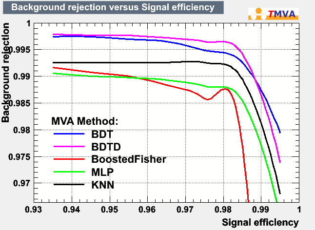
A first test was performed on a training sample based on SDSS DR7 data (Etayo-Sotos and Sevilla-Noarbe, 2013) using several of the methods described in the package, with some standard, default values. The results are shown in Figure 1 via the Receiver Operator Characteristic (ROC) curve which measures the true positive rate versus the false positive rate of the classifier for different thresholds. The BDTD method (which is a Boosted Decision Tree with a prior step of input feature decorrelation) turns out to have the best performance for this problem and training set. The decorrelation step takes care of linear correlations between the input features (vector ) by computing the square root of their covariance matrix and constructing a new input feature vector . The other standard methods which were compared are:
-
1.
k-Nearest Neighbors (kNN): a method which searches for the k closest training events in feature space.
-
2.
Fisher Discriminant (BoostedFisher): a linear discriminant analysis in which an axis in feature hyperspace is determined so that signal and background are as separated as possible.
-
3.
Neural Network (MLP): a multi-layer standard perceptron implementation of this classic technique, in which a non-linear mapping of the input feature vector is done onto a one-dimensional space as well. This is done through a complex mesh of cells which react to the input variables and modify their final classification accordingly.
This result, coupled with the success of this specific implementation in recent particle physics literature, pushed us to choose this machine learning algorithm for our tests.
Random Forests are a particularly successful technique too in the field of classification and regression in astronomy (see, e.g., Carrasco Kind and Brunner (2013)). They have better generalization properties as they can account for some scatter from the training set to the application set. On the other hand, AdaBoost BDTs can outperform slightly if the training set is representative enough. In recent tests with photometric data both give similar performances for classification (I.Sevilla-Noarbe and the DES Collaboration, in prep. and AlSayyad et al. (2015) as well as Y.Al-Sayyad, private communication). For supernovae candidate identification, random forests and boosted decision trees also compete for best performance with variable results (see Bailey et al. (2007) or Goldstein et al. in prep.).
3 Dataset
We have used this implementation of BDTs on Data Release 9 (DR9) of the Sloan Digital Sky Survey (SDSS) (Ahn et al., 2012)). The data was downloaded using the DR9 Catalog Archive Server making a selection on modelmag_r from 14 to 23 and using only spectroscopically matched objects from the photometric table, to provide a truth value for the purposes of evaluating the algorithm.
Several shape features in the -band and several magnitude measurements in all bands for bands have been used.
We have limited the shape information to only one band as, in first approximation, the values for these parameters across bands should be quite compatible. With respect to flux information, we have used a range of different magnitude types (fiber, model, petro, psf) for bands .
Finally, we include the photometric SDSS classification (type) for the object, as well as the spectroscopic classification (class) which we use as the reference (truth) value for performance in terms of purity and completeness for this work.
In Table 1 we summarize all the photometric catalog features used. The specific selection is provided in the Appendix and the resulting catalogs provides a total number of 2195172 objects.
| Parameter | Type | Description | ||
|---|---|---|---|---|
| petroR50_r | Shape |
|
||
| petroR90_r | Shape |
|
||
| lnlstar_r | Shape |
|
||
| lnlexp_r | Shape |
|
||
| lnldev_r | Shape |
|
||
| me1_r | Shape | Ellipticity component 1 | ||
| me2_r | Shape | Ellipticity component 2 | ||
| mrrcc_r | Shape | Sum of second moments of object | ||
| fibermag_[ugriz] | Magnitude |
|
||
| petromag_[ugriz] | Magnitude | Petrosian magnitude in each band | ||
| modelmag_[ugriz] | Magnitude |
|
||
| psfmag_[ugriz] | Magnitude | Magnitude as measured using the local PSF | ||
| mag_[u]-mag_[g] | Color | color | ||
| mag_[g]-mag_[r] | Color | color | ||
| mag_[r]-mag_[i] | Color | color | ||
| mag_[i]-mag_[z] | Color | color |
One of the reasons for choosing this range of magnitudes and features is also to allow for an easier comparison with the performances quoted by (Vasconcellos et al., 2011), which we have used as reference. In this case, the authors performed a thorough testing of different Decision Tree flavors. The original AdaBoost Boosted Decision Tree implementation we chose is not contemplated in their study, and we will quantitatively compare the results obtained, though our goal is to understand the impact of different choices of features and training set characteristics.
We randomly sampled the resulting catalog into training, evaluation and test samples.
-
1.
200000 objects went into the training sample to have a variety of smaller training sets and measure training sample size dependency. From this sample, the TMVA framework (see Section 4) uses a specified amount for actual training. This is useful for the comparison of different codes in the same execution.
-
2.
800000 objects went into the evaluation sample, which we use to optimize the classifier parameters.
-
3.
The rest (1195172) conform the testing sample which is the one actually used to evaluate real performance.
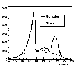
In Figure 2 the magnitude distribution for the objects in the catalog is shown, in this case, for the training set (same relative distributions as for the evaluation and testing sets).
4 Methodology
To measure performance, we define the efficiency (E) and impurity (I) of the galaxy sample as:
| (4) |
| (5) |
where (, ) is the number of true (stars, galaxies) selected by the classifier at magnitude and corresponds to the total sample of true galaxies. True stars and galaxies are determined according to its spectral classification in the SDSS catalog via the class parameter.
These metrics show a method of direct comparison against science case requirements, usually expressed in these terms (or, equivalently, completeness and purity). In our case, we will be concerned with obtaining the lowest impurity from stars possible in our galaxy sample, given a fixed efficiency value.
To optimize and test the behavior of this classifier, we have followed these steps:
-
1.
Train and evaluate on the training and evaluation sets in a grid of BDT parameters. Select best set in terms of performance (impurity level for a given efficiency).
-
2.
Evaluate the performance on the evaluation set for different training set sizes and depths, as well as the computation times.
-
3.
Test the chosen configuration against the photometric type performance provided by the SDSS catalogs with the test set.
-
4.
Verify the impact of a different choice of features assuming the same parameters and training set size are valid. We will implicitly assume here the independence of the BDT parameters with respect to these choices.
The BDT parameters to be tuned are described below. The values of the grid are shown in Table 2, based on previous experience (Etayo-Sotos and Sevilla-Noarbe, 2013):
-
1.
ntrees: Number of decision trees involved in the computation.
-
2.
nevmin: Minimum number of events held in a leaf.
-
3.
maxdepth: Maximum size of the tree, in terms of steps from the first decision.
-
4.
ncuts: Number of bins used for the cuts in each feature being tested.
| Parameter | Range |
|---|---|
| ntrees | 200,400,1000,2000,3000 |
| nevmin | 10,50,100,400,1000 |
| maxdepth | 5,10,15,20,30 |
| ncuts | 20,50,200,500,1000 |
This grid was explored by submitting multiple batch jobs to a cluster both for the training and evaluation sets, as defined in Section 3. We have narrowed down to this particular set of values in each case after a test in a wider range, the limits being imposed by performance and relative gain with respect to execution time.
The computation was performed using the Euler cluster at the CIEMAT Spanish national lab, in Madrid. This cluster is composed of 144 nodes with 2GB RAM and two Quad-core Xeon processors each at 3.0 GHz clock speed.
5 Results and discussion
We will now use the impurity metric defined in equation 5 as the value to compare the performance of each Boosted Decision Tree set we produce, as well as for the SDSS type parameter. In order to compare fairly with the latter we have adjusted the selection cut for each BDT so that its efficiency (equation 4) was within of the efficiency found for the type classifier at that particular magnitude bin (in modelmag_r).
In this section we detail the strategy to select the parameters for the BDT, as well as the impact of a varying training set size, composition, depth and feature selection, which can also provide hints for the expected performance of other machine learning methods which extract the same information and relationships in the data.
5.1 Selection of optimal parameters for the BDTs
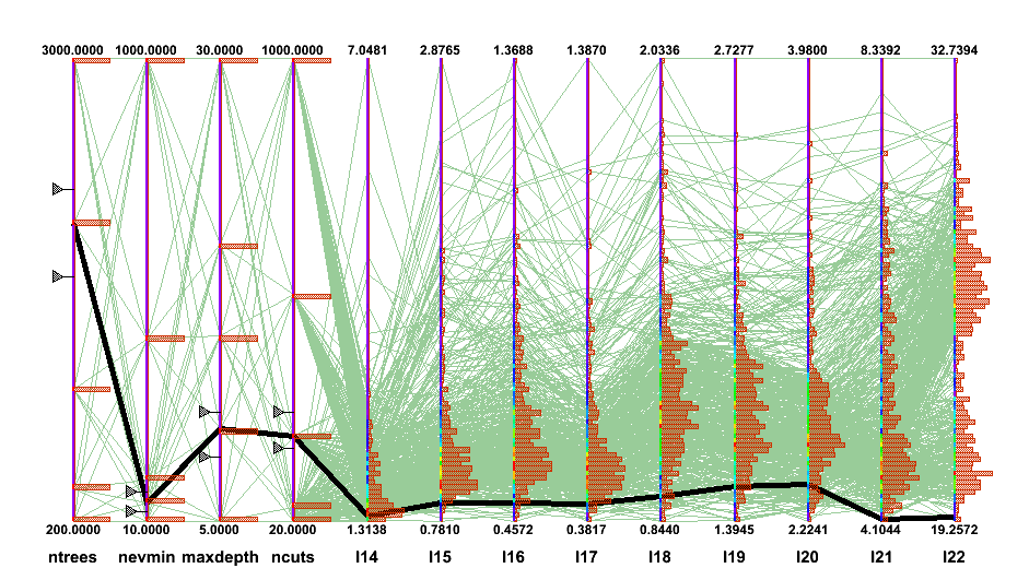
We have executed the 625 jobs of the parameter grid, corresponding to all combinations of parameters in Table 2), and obtained a 9-element vector with the impurity level for each magnitude bin (modelmag in -band). We select the parameter set which provides the best (lowest) overall impurity level in the evaluation set (boldface in Table 2). In order to do so, we visualize the performance of all possible combinations through a parallel coordinates plot such as the one shown in Figure 3. This type of representation allows showing a set of points in a N-dimensional space, with four input parameters and a 9-component vector output, so that N lines are drawn, each encompassing the whole range of each input and output value. A point in this N-dimensional space is represented as a polyline with vertices on the parallel axes. In our case, the first four points connected by the polyline represent the input parameter values of Table 2, and are connected by continuing the polyline to the 9-output components of the impurity vector, which is the metric we are using. With this tool, it is possible to distinguish the overall performance of a particular combination of input values for the parameters against the background of other possible combinations. In the figure, the specific combination which provides a good overall impurity level throughout the magnitude range is shown with a thicker line. This combination is highlighted in boldface in Table 2.
Examples of the effect of the change of specific features are shown in Figure 4. The increase in the number of trees, tree depth and number of cuts in each feature decrease the impurity level achieved until a certain stable value beyond which there is no significant gain though we incur in an execution time penalization as well as increasing the risk of overfitting (although the boosting approach tries to avoid this).

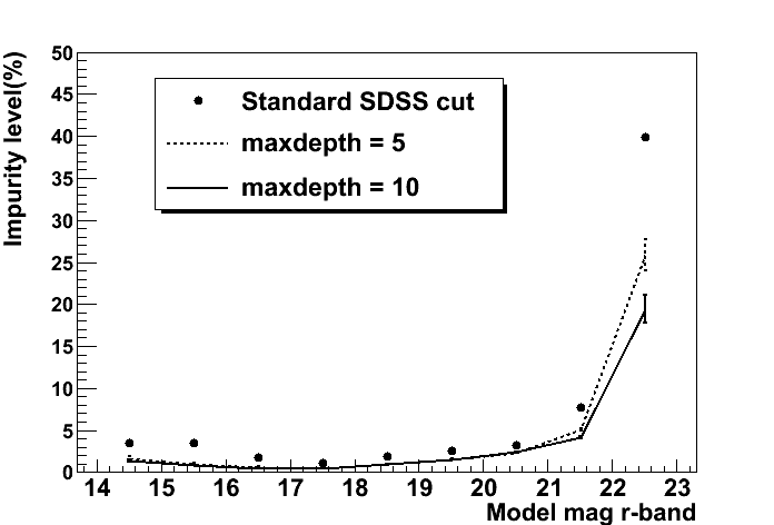
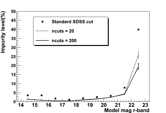
The training set size used was subselected to include 30000 randomly-picked galaxies and 6000 stars likewise chosen. This size provides a suitable trade-off between computation time and training performance. We will show in Section 5.2 the results when these values are modified.
5.2 Dependence with training set size
The number of samples, both for signal and background, is directly related to the performance of the classifier, as an increasingly varied array of galaxy and star types are covered. The fact that we have used an unbiased sample, in the sense that no targeting has been specifically done for these objects, and covering a wide area, which diminishes the impact of sample variance, makes this catalog an exceptional resource, up to the available depth. These characteristics allow us to understand the impact of the training sample solely in terms of its size, without worrying about the specific kinds of objects which populate the sample.
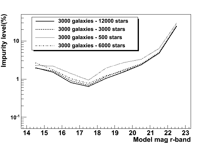
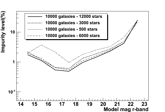
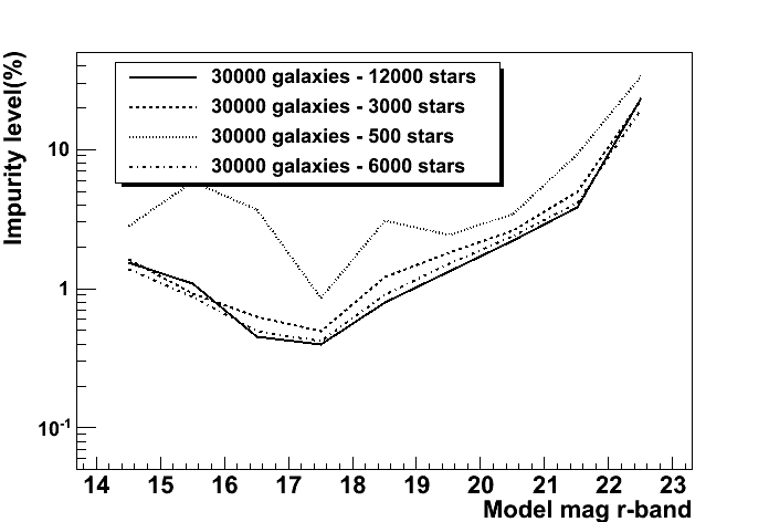
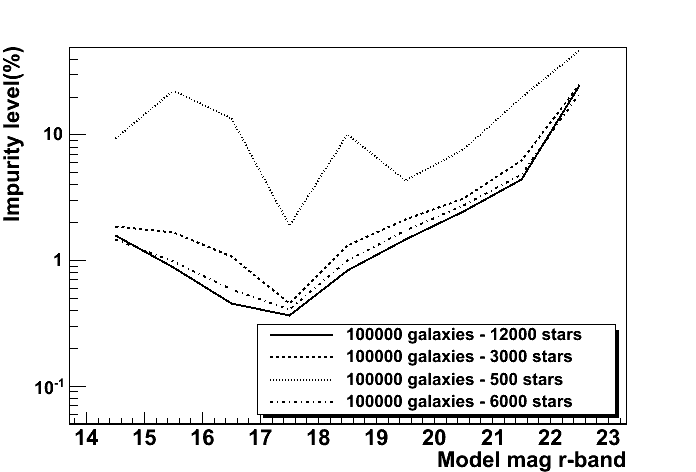
In Figure 5 we show the evolution of the impurity level (our chosen comparison metric) with respect to the size of the training set, as well as the relative mixing of galaxies and stars. In Table 3 the training times for different source and background sample sizes are shown.
By studying both results, a good compromise in terms of speed and impurity metric is the choice of using 30000 galaxies and 6000 stars. Increasing the number of galaxies does not improve things much and on the other hand, not providing sufficient number of stars to have a well balanced sample can ruin our impurity performance, as the classifier will tend to classify objects as galaxies. This can be seen in the lower right panel of Figure 5 or in any panel, when the available star sample is only populated by 500 objects, leaving a small star-to-galaxy ratio which will tend to make objects to be classified predominantly as galaxies, as some specific stellar types may have been randomly left out or are underrepresented.
Note well that the process of selecting the most adequate training set size and mix, as well as the one with best performance (Section 5.1) has been through an iterative process in which a default set of parameters were used with varying sample size, then the most adequate parameters were chosen, again training sample size sensitivity was reanalyzed, etc.
| Training time (s) | Nb. Galaxies in training | ||||
|---|---|---|---|---|---|
| Nb. stars in training | 1000 | 3000 | 10000 | 30000 | 100000 |
| 500 | 36 | 89 | 201 | 599 | 2550 |
| 3000 | 118 | 203 | 280 | 709 | 2980 |
| 6000 | 253 | 346 | 355 | 795 | 3030 |
| 12000 | 547 | 322 | 489 | 1160 | 3230 |
5.3 Dependence with training set depth
A common circumstance that many present and future photometric surveys will face is the lack of adequate training for their machine learning based classifiers, due to the unavailability of overlapping areas with spectroscopic information reaching the full survey depth. In this section, we experiment with variations in the availability of training samples depending on the magnitude limit we impose to them, and verify the impact on the impurity of the galaxy sample.
In Figure 6 the results for different choice of training depths are shown.
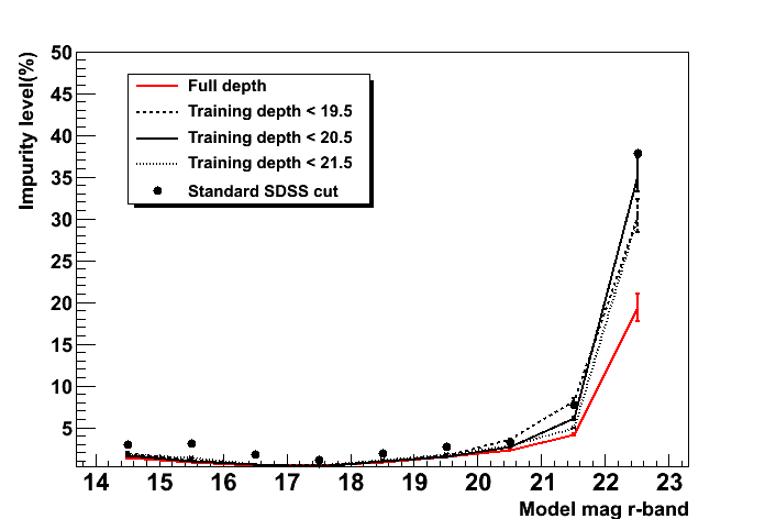
It can be verified that such variations are indeed significant and more important specially at magnitudes deeper than where training was available. In fact, a morphological cut approach, such as the SDSS photometric type can be as valid as a machine learning method employing multiple features, if the training is not deep enough.
5.4 Dependence with features
It is interesting to explore what the different features from Table 1 contribute to the overall result. We separate for this study the available features into shape-related, magnitude-related and color-related, as specified on the second column of the aforementioned table.
In Figure 7 the impact of different choice of features are shown.
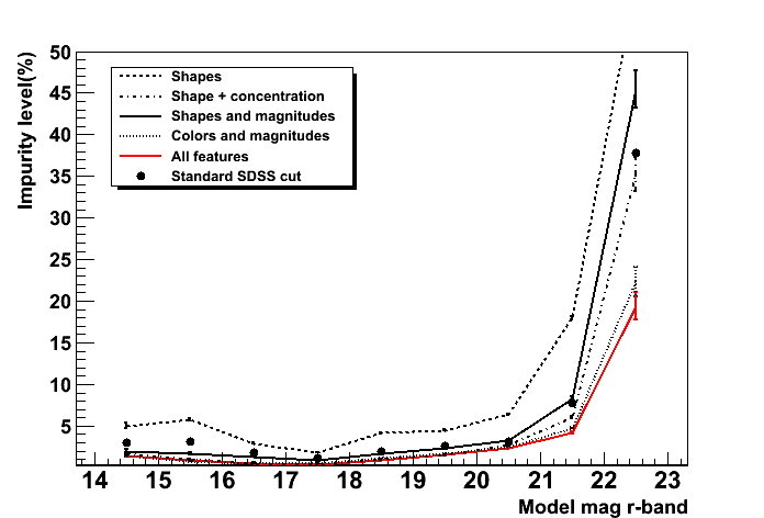
Color and magnitude information are clearly the most important sources from which the BDTs cull their information. Using shape features (light radii, ellipticity, fit likelihoods to models), on the other hand, cannot compete with the clues provided by a concentration parameter, which proves to be a robust measurement. Indeed, adding this combination to the shape input features is an important improvement to the classifier, and provides a similar response. Therefore, when using single band information, a simple cut on a ’concentration’-like parameter (e.g. differences in fluxes from PSF magnitudes and model magnitudes, or the SPREAD_MODEL parameter showcased in Desai et al. (2012) and Soumagnac et al. (2015)) should be enough.
5.5 Evaluation against SDSS DR9 photometric type
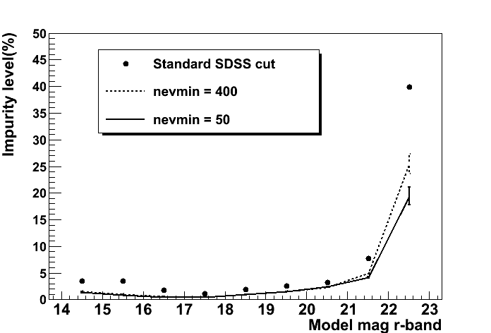
To test independently of the training and evaluation set, we have used the test set, with the chosen parameters and training size. The results are shown in in Figure 8, to be compared with the results for the photometric type provided with the catalog. This classifier has a similar performance to the standard psfmag-cmodelmag cut222https://www.sdss3.org/dr8/algorithms/classify.php. Our suggested BDT approach provides an improvement of 2 to 4 times on the impurity level, with this relatively simple training approach, using color, magnitude and shape information.
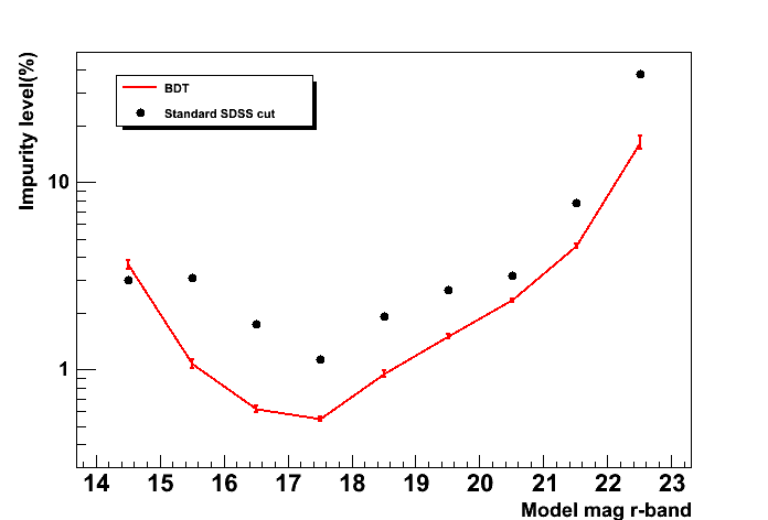
We can compare our results with the ones reported by Vasconcellos et al. (2011) by fixing the efficiency values to approximately the same ones they show in Figure 6 of their paper. We obtain impurity levels around or below (except of at the magnitude bin of 14-15), maybe slightly smaller than what it is shown for their DT classifier. However, their dataset is shallower, and their choice of parameters is morphological, further evidencing the conclusions of our work in terms of dependency of performance with depth and feature selection.
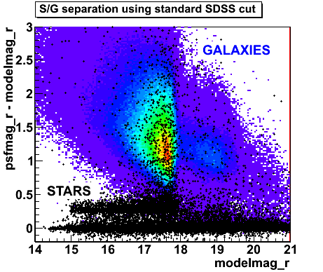
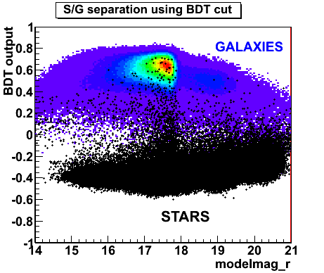
The separation power of the BDT method can be qualitatively appreciated in Figure 9.
6 Conclusions
In this work we have showed the improvements that we obtain by applying AdaBoost Boosted Decision Trees on SDSS DR9 photometric data to classify objects as stars or galaxies, using colors as well as morphological features, using a prior feature decorrelation step. This technique, very successful in other fields akin to astrophysics, has never been applied, to our knowledge, for this optical astronomy application. Using spectroscopic data from the survey itself, we have tuned the parameters for best performance, and then compared against the usage of the standard type photometric parameter from the SDSS catalogs, obtaining up to a factor 4 improvement in the impurity of the galaxy sample.
In addition to this we have made a few variations on the training sample to verify the impact on the classification. These results have general validity for other machine learning classifiers, which rely on the same available catalog information.
The BDT parameter choice has been done scanning through different values, and using different training set sizes. Using a parallel coordinates plot for this kind of analysis has proven to be a very simple and useful tool which is widely extensible to other machine learning approaches. For this unbiased sample, which would cover a varied array of galactic and stellar types, we notice that beyond 30k objects for training, the improvement is not relevant.
Training set mixture is a desirable feature of the training set, as too many galaxies in the sample tend to fool the classifier oftentimes into assigning stars as galaxies. Therefore, a relevant presence of background objects (in our case, at least 20%) is necessary to ensure an applicable training.
Colors and magnitudes are the most important features used by the BDTs to improve the performance over the morphology-based SDSS type, though the latter, proves to be a simple and robust figure (based on concentration of light) which is easy to implement and can be sufficient for many studies, as has been proven in the literature. Using light concentration together with shape information in this machine learning implementation simply converges to the standard type classification. It is the addition of information of color space that gives the additional edge.
Extensions to this work include new object types such as quasars (more relevant on next generation deeper surveys) or image artifacts. Including photometric redshift as an input feature is also an alternative avenue to pursue as a ’color’ selection. Finally, a veritable improvement of this classifier would be incorporating it into a Bayesian framework. This way, the computation of correlation functions for example, that made use of the survey galaxies would not have to have a sample previously selected, but incorporate all objects with an associated probability. See for example Fadely et al. (2012), Carrasco Kind and Brunner (2014), Kim et al. in prep. This would be an asset too for weak lensing measurements, in which a contamination of the shear catalog by stars introduces an additive bias in the shear-shear correlation function (E. Sheldon, private communication).
The code used is made available333http://github.com/nsevilla/BDT_sg_classification with this publication. I requires previous installation of the ROOT framework444http://root.cern.ch. We used version 5.18 for all our tests. The dataset can be downloaded using the query in the Appendix and is also available online555http://wwwae.ciemat.es/sevilla/bdts.
7 Acknowledgements
ISN would like to thank Robert Brunner, Alex Drlica-Wagner and O.Peña for useful discussions in the development and testing of this code, as well as for insights into its usage.
We thank the Spanish Ministry of Economy and Competitiveness (MINECO) for funding support through grant FPA2013-47986-C3-2-P.
Appendix: Query to obtain the catalog
SELECT
p.ra, p.dec
p.petromag_u, p.petromag_g, p.petromag_r, p.petromag_i,
p.petromag_z, p.modelmag_u, p.modelmag_g, p.modelmag_r,
p.modelmag_i, p.modelmag_z, p.psfmag_u, p.psfmag_g,
p.psfmag_r, p.psfmag_i, p.psfmag_z, p.fibermag_u,
p.fibermag_g, p.fibermag_r, p.fibermag_i, p.fibermag_z,
p.petrorad_r, p.petror50_r, p.petror90_r, p.lnlstar_r, p.lnlexp_r,
p.lnldev_r, p.me1_r, p.me2_r, p.mrrcc_r, s.class
into mydb.SGtable
from dr9.PhotoPrimary
AS p
JOIN dr9.SpecObj
AS s
ON s.bestobjid = p.objid
WHERE p.modelmag_r between 14.0 and 23.0
References
- Aguilar et al. (2013) Aguilar, M., Alberti, G., Alpat, B., Alvino, A., Ambrosi, G., Andeen, K., Anderhub, H., Arruda, L., Azzarello, P., Bachlechner, A., et al., 2013. First Result from the Alpha Magnetic Spectrometer on the International Space Station: Precision Measurement of the Positron Fraction in Primary Cosmic Rays of 0.5-350 GeV. Physical Review Letters 110, 141102. doi:10.1103/PhysRevLett.110.141102.
- Ahn et al. (2012) Ahn, C.P., Alexandroff, R., Allende Prieto, C., Anderson, S.F., Anderton, T., Andrews, B.H., Aubourg, É., Bailey, S., Balbinot, E., Barnes, R., et al., 2012. The Ninth Data Release of the Sloan Digital Sky Survey: First Spectroscopic Data from the SDSS-III Baryon Oscillation Spectroscopic Survey. The Astrophysical Journal Supplements Series 203, 21. doi:10.1088/0067-0049/203/2/21, arXiv:1207.7137.
- AlSayyad et al. (2015) AlSayyad, Y., McGreer, I.D., Fan, X., Connolly, A.J., Ivezic, Z., Becker, A.C., 2015. Optical Variability and Classification of High Redshift (3.5 < z < 5.5) Quasars on SDSS Stripe 82, in: American Astronomical Society Meeting Abstracts, p. 144.46.
- Bailey et al. (2007) Bailey, S., Aragon, C., Romano, R., Thomas, R.C., Weaver, B.A., Wong, D., 2007. How to Find More Supernovae with Less Work: Object Classification Techniques for Difference Imaging. The Astrophysical Journal 665, 1246--1253. doi:10.1086/519832, arXiv:0705.0493.
- Ball et al. (2006) Ball, N.M., Brunner, R.J., Myers, A.D., Tcheng, D., 2006. Robust Machine Learning Applied to Astronomical Data Sets. I. Star-Galaxy Classification of the Sloan Digital Sky Survey DR3 Using Decision Trees. The Astrophysical Journal 650, 497--509. doi:10.1086/507440, arXiv:astro-ph/0606541.
- Bertin and Arnouts (1996) Bertin, E., Arnouts, S., 1996. SExtractor: Software for source extraction. Astronomy & Astrophysics 117, 393--404.
- Brun and Rademakers (1997) Brun, R., Rademakers, F., 1997. ROOT: An object oriented data analysis framework. Nuclear Instruments and Methods in Physics Research A 389, 81--86. doi:10.1016/S0168-9002(97)00048-X.
- Carrasco Kind and Brunner (2013) Carrasco Kind, M., Brunner, R.J., 2013. TPZ: photometric redshift PDFs and ancillary information by using prediction trees and random forests. Monthly Notices of the Royal Astronomical Society 432, 1483--1501. doi:10.1093/mnras/stt574, arXiv:1303.7269.
- Carrasco Kind and Brunner (2014) Carrasco Kind, M., Brunner, R.J., 2014. Exhausting the information: novel Bayesian combination of photometric redshift PDFs. Monthly Notices of the Royal Astronomical Society 442, 3380--3399. doi:10.1093/mnras/stu1098, arXiv:1403.0044.
- CMS-Collaboration (2012) CMS-Collaboration, 2012. Observation of a new boson at a mass of 125 gev with the {CMS} experiment at the {LHC}. Physics Letters B 716, 30 -- 61. URL: http://www.sciencedirect.com/science/article/pii/S0370269312008581, doi:http://dx.doi.org/10.1016/j.physletb.2012.08.021.
- Coupon et al. (2012) Coupon, J., Kilbinger, M., McCracken, H.J., Ilbert, O., Arnouts, S., Mellier, Y., Abbas, U., de la Torre, S., Goranova, Y., Hudelot, P., Kneib, J.P., Le Fèvre, O., 2012. Galaxy clustering in the CFHTLS-Wide: the changing relationship between galaxies and haloes since . Astronomy & Astrophysics 542, A5. doi:10.1051/0004-6361/201117625, arXiv:1107.0616.
- Desai et al. (2012) Desai, S., Armstrong, R., Mohr, J.J., Semler, D.R., Liu, J., Bertin, E., Allam, S.S., Barkhouse, W.A., Bazin, G., Buckley-Geer, E.J., Cooper, M.C., Hansen, S.M., High, F.W., Lin, H., Lin, Y.T., Ngeow, C.C., Rest, A., Song, J., Tucker, D., Zenteno, A., 2012. The Blanco Cosmology Survey: Data Acquisition, Processing, Calibration, Quality Diagnostics, and Data Release. The Astrophysical Journal 757, 83. doi:10.1088/0004-637X/757/1/83, arXiv:1204.1210.
- Etayo-Sotos and Sevilla-Noarbe (2013) Etayo-Sotos, P., Sevilla-Noarbe, I., 2013. Using boosted decision trees for star-galaxy separation, in: Guirado, J.C., Lara, L.M., Quilis, V., Gorgas, J. (Eds.), Highlights of Spanish Astrophysics VII, pp. 944--944.
- Fadely et al. (2012) Fadely, R., Hogg, D.W., Willman, B., 2012. Star-Galaxy Classification in Multi-band Optical Imaging. The Astrophysical Journal 760, 15. doi:10.1088/0004-637X/760/1/15, arXiv:1206.4306.
- Fermi-LAT-Collaboration (2012) Fermi-LAT-Collaboration, 2012. A Statistical Approach to Recognizing Source Classes for Unassociated Sources in the First Fermi-LAT Catalog. The Astrophysical Journal 753, 83. doi:10.1088/0004-637X/753/1/83, arXiv:1108.1202.
- Freund and Schapire (1997) Freund, Y., Schapire, R.E., 1997. A decision-theoretic generalization of on-line learning and an application to boosting. Journal of Computer and System Sciences 55, 119 -- 139. URL: http://www.sciencedirect.com/science/article/pii/S002200009791504X, doi:http://dx.doi.org/10.1006/jcss.1997.1504.
- Gerdes et al. (2010) Gerdes, D.W., Sypniewski, A.J., McKay, T.A., Hao, J., Weis, M.R., Wechsler, R.H., Busha, M.T., 2010. ArborZ: Photometric Redshifts Using Boosted Decision Trees. The Astrophysical Journal 715, 823--832. doi:10.1088/0004-637X/715/2/823, arXiv:0908.4085.
- Giannantonio et al. (2014) Giannantonio, T., Ross, A.J., Percival, W.J., Crittenden, R., Bacher, D., Kilbinger, M., Nichol, R., Weller, J., 2014. Improved primordial non-Gaussianity constraints from measurements of galaxy clustering and the integrated Sachs-Wolfe effect. Physical Review D 89, 023511. doi:10.1103/PhysRevD.89.023511, arXiv:1303.1349.
- Heydon-Dumbleton et al. (1989) Heydon-Dumbleton, N.H., Collins, C.A., MacGillivray, H.T., 1989. The Edinburgh/Durham Southern Galaxy Catalogue. II - Image classification and galaxy number counts. Monthly Notices of the Royal Astronomical Society 238, 379--406.
- Hildebrandt et al. (2012) Hildebrandt, H., Erben, T., Kuijken, K., van Waerbeke, L., Heymans, C., et al., 2012. CFHTLenS: Improving the quality of photometric redshifts with precision photometry. Mon.Not.Roy.Astron.Soc. 421, 2355. doi:10.1111/j.1365-2966.2012.20468.x, arXiv:1111.4434.
- Hoecker et al. (2007) Hoecker, A., Speckmayer, P., Stelzer, J., Therhaag, J., von Toerne, E., Voss, H., 2007. TMVA: Toolkit for Multivariate Data Analysis. PoS ACAT, 040. arXiv:physics/0703039.
- MacGillivray et al. (1976) MacGillivray, H.T., Martin, R., Pratt, N.M., Reddish, V.C., Seddon, H., Alexander, L.W.G., Walker, G.S., Williams, P.R., 1976. A method for the automatic separation of the images of galaxies and stars from measurements made with the COSMOS machine. Monthly Notices of the Royal Astronomical Society 176, 265--274.
- Maddox et al. (1990) Maddox, S.J., Efstathiou, G., Sutherland, W.J., Loveday, J., 1990. The APM galaxy survey. I - APM measurements and star-galaxy separation. Monthly Notices of the Royal Astronomical Society 243, 692--712.
- Małek et al. (2013) Małek, K., Solarz, A., Pollo, A., Fritz, A., Garilli, B., Scodeggio, M., Iovino, A., Granett, B.R., Abbas, U., Adami, C., Arnouts, S., Bel, J., Bolzonella, M., Bottini, D., Branchini, E., Cappi, A., Coupon, J., Cucciati, O., Davidzon, I., De Lucia, G., de la Torre, S., Franzetti, P., Fumana, M., Guzzo, L., Ilbert, O., Krywult, J., Le Brun, V., Le Fevre, O., Maccagni, D., Marulli, F., McCracken, H.J., Paioro, L., Polletta, M., Schlagenhaufer, H., Tasca, L.A.M., Tojeiro, R., Vergani, D., Zanichelli, A., Burden, A., Di Porto, C., Marchetti, A., Marinoni, C., Mellier, Y., Moscardini, L., Nichol, R.C., Peacock, J.A., Percival, W.J., Phleps, S., Wolk, M., Zamorani, G., 2013. The VIMOS Public Extragalactic Redshift Survey (VIPERS). A support vector machine classification of galaxies, stars, and AGNs. Astronomy & Astrophysics 557, A16. doi:10.1051/0004-6361/201321447, arXiv:1303.2621.
- Miller and Coe (1996) Miller, A.S., Coe, M.J., 1996. Star/galaxy classification using Kohonen self-organizing maps. Monthly Notices of the Royal Astronomical Society 279, 293--300.
- Odewahn et al. (1992) Odewahn, S.C., Stockwell, E.B., Pennington, R.L., Humphreys, R.M., Zumach, W.A., 1992. Automated star/galaxy discrimination with neural networks. Astronomical Journal 103, 318--331. doi:10.1086/116063.
- Roe et al. (2005) Roe, B.P., Yang, H.J., Zhu, J., Liu, Y., Stancu, I., McGregor, G., 2005. Boosted decision trees as an alternative to artificial neural networks for particle identification. Nuclear Instruments and Methods in Physics Research Section A: Accelerators, Spectrometers, Detectors and Associated Equipment 543, 577 -- 584. URL: http://www.sciencedirect.com/science/article/pii/S0168900205000355, doi:http://dx.doi.org/10.1016/j.nima.2004.12.018.
- Ross et al. (2011) Ross, A.J., Ho, S., Cuesta, A.J., Tojeiro, R., Percival, W.J., Wake, D., Masters, K.L., Nichol, R.C., Myers, A.D., de Simoni, F., Seo, H.J., Hernández-Monteagudo, C., Crittenden, R., Blanton, M., Brinkmann, J., da Costa, L.A.N., Guo, H., Kazin, E., Maia, M.A.G., Maraston, C., Padmanabhan, N., Prada, F., Ramos, B., Sanchez, A., Schlafly, E.F., Schlegel, D.J., Schneider, D.P., Skibba, R., Thomas, D., Weaver, B.A., White, M., Zehavi, I., 2011. Ameliorating systematic uncertainties in the angular clustering of galaxies: a study using the SDSS-III. Monthly Notices of the Royal Astronomical Society 417, 1350--1373. doi:10.1111/j.1365-2966.2011.19351.x, arXiv:1105.2320.
- Sebok (1979) Sebok, W.L., 1979. Optimal classification of images into stars or galaxies - A Bayesian approach. Astronomical Journal 84, 1526--1536. doi:10.1086/112570.
- Soumagnac et al. (2015) Soumagnac, M.T., Abdalla, F.B., Lahav, O., Kirk, D., Sevilla, I., Bertin, E., Rowe, B.T.P., Annis, J., Busha, M.T., Da Costa, L.N., Frieman, J.A., Gaztanaga, E., Jarvis, M., Lin, H., Percival, W.J., Santiago, B.X., Sabiu, C.G., Wechsler, R.H., Wolz, L., Yanny, B., 2015. Star/galaxy separation at faint magnitudes: application to a simulated Dark Energy Survey. Monthly Notices of the Royal Astronomical Society 450, 666--680. doi:10.1093/mnras/stu1410, arXiv:1306.5236.
- Suchkov et al. (2005) Suchkov, A.A., Hanisch, R.J., Margon, B., 2005. A Census of Object Types and Redshift Estimates in the SDSS Photometric Catalog from a Trained Decision Tree Classifier. Astronomical Journal 130, 2439--2452. doi:10.1086/497363, arXiv:astro-ph/0508501.
- Thomas et al. (2011) Thomas, S.A., Abdalla, F.B., Lahav, O., 2011. Excess Clustering on Large Scales in the MegaZ DR7 Photometric Redshift Survey. Physical Review Letters 106, 241301. doi:10.1103/PhysRevLett.106.241301, arXiv:1012.2272.
- Vasconcellos et al. (2011) Vasconcellos, E.C., de Carvalho, R.R., Gal, R.R., LaBarbera, F.L., Capelato, H.V., Frago Campos Velho, H., Trevisan, M., Ruiz, R.S.R., 2011. Decision Tree Classifiers for Star/Galaxy Separation. Astronomical Journal 141, 189. doi:10.1088/0004-6256/141/6/189, arXiv:1011.1951.
- Weir et al. (1995) Weir, N., Fayyad, U.M., Djorgovski, S., 1995. Automated Star/Galaxy Classification for Digitized Poss-II. Astronomical Journal 109, 2401. doi:10.1086/117459.
- Yang et al. (2005) Yang, H.J., Roe, B.P., Zhu, J., 2005. Studies of boosted decision trees for miniboone particle identification. Nuclear Instruments and Methods in Physics Research Section A: Accelerators, Spectrometers, Detectors and Associated Equipment 555, 370 -- 385. URL: http://www.sciencedirect.com/science/article/pii/S0168900205018322, doi:http://dx.doi.org/10.1016/j.nima.2005.09.022.