Google matrix of the world network of economic activities

Abstract

Using the new data from the OECD-WTO world network of economic activities we construct the Google matrix $G$ of this directed network and perform its detailed analysis. The network contains 58 countries and 37 activity sectors for years 1995 and 2008. The construction of $G$, based on Markov chain transitions, treats all countries on equal democratic grounds while the contribution of activity sectors is proportional to their exchange monetary volume. The Google matrix analysis allows to obtain reliable ranking of countries and activity sectors and to determine the sensitivity of CheiRank-PageRank commercial balance of countries in respect to price variations and labor cost in various countries. We demonstrate that the developed approach takes into account multiplicity of network links with economy interactions between countries and activity sectors thus being more efficient compared to the usual export-import analysis. The spectrum and eigenstates of $G$ are also analyzed being related to specific activity communities of countries.

1 Introduction

The recent reports of the Organisation for Economic Co-operation and Development (OECD) oecd2014 and of the World Trade Organization (WTO) wto2014 demonstrate all the complexity of global manufactoring activities, exchange and trade in the modern world. This complexity is rapidly growing with time and now it becomes clear that traditional statistics are increasingly unable to provide all the necessary information. Applying modern mathematical tools and methods to new data sets can allow to understand the hidden trends of the world economic activities. Thus the matrix tools for analysis of Input-Out transactions are broadly used in economy starting from the fundamental works of Leontief leontief1 ; leontief2 with their more recent developments described in miller2009 . In the last decade the development of modern society generated enormous communication and social networks including the World Wide Web (WWW), Wikipedia, Twitter and other directed networks (see e.g. dorogovtsev ). It has been found that the concept of Markov chains provides a very useful and powerful mathematical approach for analysis of such networks. Thus the PageRank algorithm, developed by Brin and Page in 1998 brin for the WWW information retrieval, became at the mathematical foundation of the Google search engine (see e.g. meyer ). This algorithm constructs the Google matrix $G$ of Markov chain transitions between network nodes and allows to rank billions of web pages of the WWW. The spectral and other properties of the Google matrix are analyzed in arxivrmp . The historical overviews of the development of Google matrix methods and their links with the works of Leontief are given in franceschet ; vignahisto .

The obtained results demonstrate the efficiency of the Google matrix analysis not only for the WWW but also for various types of directed networks arxivrmp . One of such examples is the World Trade Network (WTN) with multiproduct exchange between the world countries. The data of trade flows are available at the United Nations (UN) COMTRADE database comtrade for more than $50$ years. The results presented in wtngoogle ; wtnproducts for the WTN show that the Google matrix analysis is well adapted to the ranking of world countries and trade products and to determination of the sensitivity of trade to price variations of various products. The new element of such an approach is a democratic treatment of world countries independently of their richness being different from the usual Import and Export ranking. At the same time the contributions of various products are considered being proportional to their trade volume contribution in the exchange flows.

Here we use the Google matrix analysis developed for the multiproduct WTN wtnproducts showing that it can be directly used for the World Network of Economic Activities (WNEA) constructed from the OECD-WTO trade in value-added database. In a certain sense activities (or sectors) are correlated to products in the WTN. However, for the WTN there is exchange between countries but there is no exchange between industries and commodities. Thus in wtnproducts it was argued that certain economical features are not captured by the COMTRADE database since in real economy the traders are industries, not countries; in particular certain products are transferred to each other (e.g. metal and plastic are used for production of cars). In contrast to that, the OECD-WTO WNEA incorporates the transitions between activity sectors thus representing the economic reality of world activities in a more correct manner.

Figure 1: World map of countries with color showing country import (top panel) and export (bottom panel) with economic activity (trade) volume expressed in billions of USD and given by numbers at color bars; the gray color marks countries attributed to the ROW group (rest of the world) with exchange values $733$ (Import) and $1018$ (Export) in billions of USD. The data are shown for year 2008 with $N_{c}=57+1$ countries (with ROW) for the economic activities in all $N_{s}=37$ sectors. Country names can be found in Table 1 and in the world map of countries worldmap .

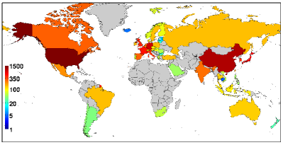
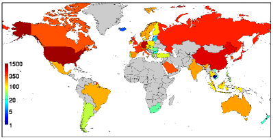
We note that there has been a number of other investigations of the WTN reported in garlaschelli ; hedeem ; fagiolo2 ; garlaschelli2010 ; benedictis ; plosjapan ; imfpaper . However, in this work we have the new important elements, introduced in wtngoogle ; wtnproducts : the analysis of PageRank and CheiRank probabilities corresponding to direct and inverted network flows and related to Import and Export; democratic treatment of countries combined with the contributions of sectors (or products) being proportional to their commercial exchange fractions. We point that the OECD-WTO TiVA database of economic activities between world countries and activity sectors has been created very recently (2013) and thus this work represents the first Google matrix analysis of these data. We stress that the usual Import-Export ranking of commercial flows, shown in Fig. 1, is not able to take into account all the complexity of chains of links between various countries and various activity sectors. In contrast to that the approach developed here takes all of them into account due to the powerful method based on the Google matrix.

2 Methods and data description

Here we describe the data available for the OECD-WTO TiVA network and the mathematical methods used for the analysis of this network. The list of $N_{c}=58$ countries ($57$ plus $1$ for the Rest Of the World ROW) is given in Table 1 with their flags. Following wtngoogle we use for countries ISO 3166-1 alpha-3 code available at Wikipedia. The list of sectors with their names is given in Table 2 . The fractions of sectors in the exchange volume are given in Table 3 for years $1995$, $2008$.

2.1 Google matrix construction for the OECD-WTO WNEA

We use the OECD-WTO TiVA database released in May 2013 which covers years $1995$, $2000$, $2005$, $2008$, $2009$ with the main emphasis for years $1995and2008$ (2009 data are affected by the global crisis and may not be representative). The network considers $N_{c}=58$ world countries given in Table 1. In fact, there are $57$ countries and the rest of the world, which includes the remaining countries of the world forming one group called ROW. There are also $N_{s}=37$ sectors of economic activities given in Table 2. The sectors are classified according to the International Standard Industrial Classification of All Economic Activities (ISIC) Rev.3 isic . Here we present results for all $37$ sectors of Table 2, noting that the sectors $s=1,2,..20$ represent production activities while $s=21,...,37$ represent service activities. The transections between service sectors are hard to exctract and the future improvements of this part of TiVA database are desirable.

For a given year, the TiVA data extend OECD Input/Out tables of economic activity expressed in terms of USD for a given year. From these data we construct the matrix $M_{cc^{\prime},ss^{\prime}}$ of money transfer between nodes expressed in USD:

$$M_{cc^{\prime},ss^{\prime}}=\text{transfer from country $c^{\prime}$, sector $s^{\prime}$ to $c,s$}$$ (1)

Here the country indexes are $c,c^{\prime}=1,\ldots,N_{c}$ and activity sector indexes are $s,s^{\prime}=1,\ldots,N_{s}$ with $N_{c}=58$ and $N_{s}=37$. The whole matrix size is $N=N_{c}\times N_{s}=2146$. Here each node represents a pair of country and activity sector, a link gives a transfer from a sector of one country to another sector of another country. We construct the matrix $M_{cc^{\prime},ss^{\prime}}$ from the TiVA Input/Output tables using the transposed representation so that the volume of products or sectors flows in a column from line to line. In the construction of $M_{cc^{\prime},ss^{\prime}}$ we exclude exchanges inside a given country in order to highlight the trade exchange flows between countries (elements inside country are zeros).

The ISIC Rev.3 classification of sectors have a significant correlation with the UN Standard International Trade Classification (SITC) Rev. 1 of products used in wtnproducts . There is a clear relationship on the production side between ISIC sectors and products of the world exports (but not at import level: if all agricultural exports are produced by the agricultural sector, agricultural products will be imported by manufacturing industries such as food processing of textile and clothing). There is also another important difference: the transfer matrix from COMTRADE is diagonal in products wtnproducts (thus there is no transfer from product to product), while for the TiVA data there are transitions from one sector to another sector and thus the matrix of nominal values, in current prices, (1) is not diagonal in $s,s^{\prime}$.

For convenience of future notations we also define the value of imports $V_{cs}$ and exports $V^{*}_{cs}$ for a given country $c$ and sector $s$ as

$$V_{cs}=\sum_{c^{\prime},s^{\prime}}M_{cc^{\prime},ss^{\prime}}\,,\,\;V^{*}_{cs}=\sum_{c^{\prime},s^{\prime}}M_{{{c^{\prime}}c},{s^{\prime}}s}.$$ (2)

The import $V_{c}=\sum_{s}V_{cs}$ and export $V^{*}_{c}=\sum_{s}V^{*}_{cs}$ values for countries $c$ are shown on the world map of countries in Fig. 1 for year 2008. We note that often one uses the notion of volume of export or import (see. e.g. wtnproducts ) but from the economic view point it more correct to speak about value of export or import.

In order to compare later with the PageRank and
CheiRank probabilities we define exchange value ranks in the whole matrix space of dimension $N=N_{c}\times N_{s}$. Thus the ImportRank ($\hat{P}$) and ExportRank ($\hat{P}^{*}$) probabilities are given by the normalized import and export values

$$\hat{P}_{i}={V_{cs}}/{V}\,,\,\;\hat{P}^{*}_{i}={V^{*}_{cs}}/{V}\,,$$ (3)

where $i=s+(c-1)N_{s}$, $i=1,\ldots,N$ and the total exchange value is $V=\sum_{c,c^{\prime},s,s^{\prime}}M_{cc^{\prime},ss^{\prime}}=\sum_{c,s}V_{cs}=\sum_{cs}V^{*}_{cs}$.

The Google matrices $G$ and $G^{*}$ are defined as $N\times N$ real matrices with non-negative elements:

$$G_{ij}=\alpha S_{ij}+(1-\alpha)v_{i}e_{j}\,,\;{G^{*}}_{ij}=\alpha{S^{*}}_{ij}+(1-\alpha)v^{*}_{i}e_{j}\,,$$ (4)

where $N=N_{c}\times N_{s}$, $\alpha\in(0,1]$ is the damping factor ($0<\alpha<1$), $e_{j}$ is the row vector of unit elements ($e_{j}=1$), and $v_{i}$ is a positive column vector called a personalization vector with $\sum_{i}v_{i}=1$ meyer ; wtnproducts . We note that the usual Google matrix corresponds to a personalization vector $v_{i}=e_{i}/N$ with $e_{i}=1$. In this work, following wtngoogle ; wtnproducts , we fix $\alpha=0.5$ noting that a variation of $\alpha$ in a range $(0.5,0.9)$ does not significantly affect the probability distributions of PageRank and CheiRank vectors meyer ; arxivrmp ; wtngoogle . The choice of the personalization vector is specified below. Following wtnproducts we call this approach the Google Personalized Vector Method (GPVM).

The matrices $S$ and $S^{*}$ are built from money matrices ${M}_{cc^{\prime},ss^{\prime}}$ as

$$S_{i,i^{\prime}} = \left\{\begin{array}[]{cl}{M}_{cc^{\prime},ss^{\prime}}/V_{c^{\prime}s^{\prime}}&\text{ if }V_{c^{\prime}s^{\prime}}\neq 0\\ 1/N&\text{ if }V_{c^{\prime}s^{\prime}}=0\\ \end{array}\right.$$ (7)

$$S^{*}_{i,i^{\prime}} = \left\{\begin{array}[]{cl}M_{{c^{\prime}}c,s^{\prime}s}/V^{*}_{c^{\prime}s^{\prime}}&\text{ if }V^{*}_{c^{\prime}s^{\prime}}\neq 0\\ 1/N&\text{ if }V^{*}_{c^{\prime}s^{\prime}}=0\\ \end{array}\right.$$ (10)

where $c,c^{\prime}=1,\ldots,N_{c}$; $s,s^{\prime}=1,\ldots,N_{s}$; $i=s+(c-1)N_{s}$; $i^{\prime}=s^{\prime}+(c^{\prime}-1)N_{s}$; and therefore $i,i^{\prime}=1,\ldots,N$. Here $V_{c^{\prime}s^{\prime}}=\sum_{cs}M_{cc^{\prime},ss^{\prime}}$. The sum of elements of each column of $S$ and $S^{*}$ is normalized to unity and hence the matrices $G,G^{*},S,S^{*}$ belong to the class of Google matrices and Markov chains. Thus $S,G$ look at the import perspective and $S^{*},G^{*}$ at the export side of transactions.

PageRank and CheiRank ($P$ and $P^{*}$) are the right eigenvectors of $G$ and $G^{*}$ matrices respectively at eigenvalue $\lambda=1$. The equation for right eigenvectors have the form

$$\sum_{j}G_{ij}\psi_{j}=\lambda\psi_{i}\,,\;\sum_{j}{G^{*}}_{ij}{\psi^{*}}_{j}=\lambda{\psi^{*}}_{j}\;.$$ (11)

For the eigenstate at $\lambda=1$ we use the notation $P_{i}=\psi_{i},P^{*}={\psi^{*}}_{i}$ with the normalization $\sum P_{i}=\sum_{i}{P^{*}}_{i}=1$. For other eigenstates we use the normalization $\sum_{i}|\psi_{i}|^{2}=\sum_{i}|\psi^{*}_{i}|^{2}=1$. The eigenvalues and eigenstates of $G,G^{*}$ are obtained by a direct numerical diagonalization using the standard numerical packages.

2.2 PageRank and CheiRank vectors from GPVM

The components of $P_{i}$, ${P^{*}}_{i}$ are positive. In the WWW context they have a meaning of probabilities to find a random surfer on a given WWW node in the limit of large number of surfer jumps over network links meyer . In the WNEA context nodes can be viewed and markets with a random trader transitions between them. We will use in the following notation of netwrok nodes. We define the PageRank $K$ and CheiRank $K^{*}$ indexes ordering probabilities $P$ and $P^{*}$ in a decreasing order as $P(K)\geq P(K+1)$ and $P^{*}(K)\geq P^{*}(K^{*}+1)$ with $K,K^{*}=1,\ldots,N$.

We note that the pair of PageRank and CheiRank vectors is very natural for economy and trade networks corresponding to Import and Export flows. For the directed networks the statistical properties of the pair of such ranking vectors have been introduced and studied in linux ; wikizzs ; wtngoogle .

We compute the reduced PageRank and CheiRank probabilities of countries tracing probabilities over all sectors and getting $P_{c}=\sum_{s}P_{cs}=\sum_{s}P\left(s+(c-1)N_{s}\right)$ and $P^{*}_{c}=\sum_{s}P^{*}_{cs}=\sum_{s}P^{*}\left(s+(c-1)N_{s}\right)$ with the corresponding $K_{c}$ and $K^{*}_{c}$ indexes. In a similar way we obtain the reduced PageRank and CheiRank probabilities for sectors tracing over all countries and getting
$P_{s}=\sum_{c}P\left(s+(c-1)N_{s}\right)=\sum_{c}P_{cs}$ and
$P^{*}_{s}=\sum_{c}P^{*}\left(s+(c-1)N_{s}\right)=\sum_{c}P^{*}_{cs}$ with their corresponding sector indexes $K_{s}$ and $K^{*}_{s}$. A similar procedure has been used for the multiproduct WTN data wtnproducts .

In summary we have $K_{s},K^{*}_{s}=1,\ldots,N_{s}$ and $K_{c},K^{*}_{c}=1,\ldots,N_{c}$. A similar definition of ranks from import and export exchange value can be done in a straightforward way via probabilities $\hat{P}_{s},\hat{P}^{*}_{s},\hat{P}_{c},\hat{P}^{*}_{c},\hat{P}_{cs},\hat{P}^{*}_{cs}$ and corresponding indexes $\hat{K}_{s},\hat{K}^{*}_{s},\hat{K}_{c},\hat{K}^{*}_{c},\hat{K},\hat{K}^{*}$.

To compute the PageRank and CheiRank probabilities from $G$ and $G^{*}$, keeping a “democratic”, or equal, treatment of countries (independently of their richness) and at the same time keeping the proportionality of activity sectors to their exchange value, we use the Google Personalized Vector Method (GPVM) developed in wtnproducts with a personalized vector $v_{i}$ in (4). At the first iteration of Google matrix we take into account the relative product value per country using the following personalization vectors for $G$ and $G^{*}$:

$$v_{i}=\frac{V_{cs}}{N_{c}\sum_{s^{\prime}}V_{cs^{\prime}}}\,,\;v^{*}_{i}=\frac{V^{*}_{cs}}{N_{c}\sum_{s^{\prime}}V^{*}_{cs^{\prime}}}\,,$$ (12)

using the definitions (2) and the relation $i=s+(c-1)N_{s}$. This personalized vector depends both on sector and country indexes. As for the multiproduct WTN in wtnproducts we define the second iteration vector being proportional to the reduced PageRank and CheiRank vectors in sectors, obtained from the GPVM Google matrix of the first iteration:

$$v^{\prime}(i)=\frac{P_{s}}{N_{c}}\,,\;v^{\prime*}(i)=\frac{P^{*}_{s}}{N_{c}}\,.$$ (13)

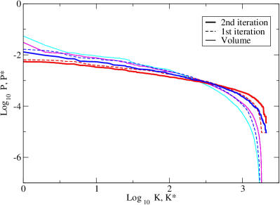
In this way we keep democracy in countries but keep contribution of sectors proportional to their exchange value. This second iteration personalized vectors are used in the following computations and operations with $G$ and $G^{*}$ giving us the PageRank and CheiRank vectors. This procedure with two iterations forms our GPVM approach. The difference between results obtained from the first and second iterations is not very large (see Figs. 2, 3), but the personalized vector for the second iteration gives a reduction of fluctuations. In all Figures after Fig. 3 we show the GPVM results after the second iteration.

Figure 2: Dependence of probabilities of PageRank $P(K)$, CheiRank $P^{*}(K^{*})$, ImportRank $\hat{P}(\hat{K})$ and ExportRank $\hat{P}^{*}(\hat{K}^{*})$ on their indexes in logarithmic scale for WNEA (or OECD-WTO TiVA network) in 2008 with $\alpha=0.5$, $N_{c}=58$, $N_{s}=37$, $N=N_{c}\times N_{s}=2146$. Here the results for the GPVM after the first and second iterations are shown for PageRank (CheiRank) in red (blue) with dashed and solid curves respectively.      Probabilities for ImportRank and ExportRank from exchange value are shown by magenta and cyan thin curves respectively.

Figure 3: Probability distributions of PageRank and CheiRank for sectors $P_{s}(K_{s})$, $P^{*}_{s}(K^{*}_{s})$ (left panel) and countries $P_{c}(K_{c})$, $P^{*}_{c}(K^{*}_{c})$ (right panel) in logarithmic scale for WNEA (or OECD-WTO TiVA network) from Fig.2. Here the results for the first and second GPVM iterations are shown by red (blue) curves for PageRank (CheiRank) with dashed and solid curves respectively (with a strong overlap of curves). The probabilities from the exchange value ranking are shown by thin magenta and cyan lines for ImportRank and ExportRank respectively.

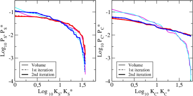
As for the WTN it is convenient to analyze the distribution of nodes on the PageRank-CheiRank plane $(K,K^{*})$. In addition to two ranking indexes $K,K^{*}$ we use also 2DRank index $K_{2}$ which describes the combined contribution of two ranks as described in wikizzs . The ranking list $K_{2}(i)$ is constructed by increasing $K\rightarrow K+1$ and increasing 2DRank index $K_{2}(i)$ by one if a new entry is present in the list of first $K^{*}<K$ entries of CheiRank, then the one unit step is done in $K^{*}$ and $K_{2}$ is increased by one if the new entry is present in the list of first $K<K^{*}$ entries of CheiRank. More formally, 2DRank $K_{2}(i)$ gives the ordering of the sequence of nodes, that   appear inside   the squares   $\left[1,1;\;K=k,K^{\ast}=k;\;\-...\right]$ when one runs progressively from $k=1$ to $N$. Additionally, we analyze the distribution of nodes for reduced indexes $(K_{c},K^{*}_{c})$, $(K_{s},K^{*}_{s})$.

The localization properties of eigenstates of $G,G^{*}$ are characterized by the inverse participation ration (IPR) defined as $\xi=(\sum_{i}|\psi_{i}|^{2})^{2}/\sum_{i}|\psi_{i}|^{4}$. This quantity determines an effective number of nodes contributing to a formation of a given eigenstate (see details in arxivrmp ).

2.3 Correlators of PageRank and CheiRank vectors

As in previous works linux ; wikizzs ; wtngoogle we consider the correlator of PageRank and CheiRank vectors:

$$\kappa=N\sum_{i=1}^{N}P(i)P^{*}(i)-1\;.$$ (14)

The typical values of $\kappa$ are given in arxivrmp for various networks.

For the global PageRank and CheiRank probabilities the sector-sector correlator matrix is defined as:

$$\kappa_{ss^{\prime}}=N_{c}\sum_{c=1}^{N_{c}}\left[\frac{P(s+(c-1)N_{s})P^{*}(s^{\prime}+(c-1)N_{s})}{\sum_{c^{\prime}}P(s+(c^{\prime}-1)N_{s})\sum_{c^{\prime\prime}}P^{*}(s^{\prime}+(c^{\prime\prime}-1)N_{s})}\right]-1$$ (15)

Then the correlator for a given sector is obtained from (15) as:

$$\kappa_{s}=\kappa_{ss^{\prime}}\delta_{s,s^{\prime}}\,,$$ (16)

where $\delta_{s,s^{\prime}}$ is the Kronecker delta.

We also use the correlators obtained from the probabilities traced over sectors ($P_{c}=\sum_{s}P_{sc}$) and over countries ($P_{s}=\sum_{c}P_{sc}$) which are defined as

$$\kappa(c)=N_{c}\sum_{c=1}^{N_{c}}P_{c}P^{*}_{c}-1\,,\;\kappa(s)=N_{s}\sum_{s=1}^{N_{s}}P_{s}P^{*}_{s}-1\,.$$ (17)

In the above equations (14)-(17) the correlators are computed for PageRank and CheiRank probabilities. We can also compute the same correlators using probabilities from the exchange value in ImportRank $\hat{P}$ and ExportRank $\hat{P}^{*}$ defined by (3).

The obtained results are presented in the next Section and at the web site ourwebpage .

3 Results

We apply the GPVM approach to the data sets of OECD-WTO TiVA of WNEA and present the obtained results below.

3.1 PageRank and CheiRank probabilities

The dependence of probabilities of PageRank $P(K)$ and CheiRank $P^{*}(K^{*})$ vectors on their indexes $K,K^{*}$ are shown in Fig. 2 for a selected year 2008. The results can be approximately described by an algebraic dependence $P\propto 1/K^{\beta}$, $P^{*}\propto 1/{K^{*}}^{\beta}$ with the fit exponent value $\beta=0.385\pm 0.014$ for PageRank and $\beta=0.486\pm 0.02$ for CheiRank for $K,K^{*}\leq 10^{3}$. In contrast to WWW and Wikipedia networks (see e.g. arxivrmp ) there is no significant difference of $\beta$ between two ranks that can be attributed to an intrinsic property of economy networks to keep economy balance of commercial exchange. The probability variation is reduced for the Google ranking compared to the value ranking. This results from a “democratic”, or equal grounds ranking of countries used in the Google matrix analysis. The obtained data also show that the variation of probabilities for 1st and 2nd GPVM iterations are not very large that demonstrates the convergence of this approach.

Figure 4: Country positions on PageRank-CheiRank plane ($K_{c}$,$K^{*}_{c}$) obtained for the WNEA by the GPVM analysis (top panels), ImportRank-ExportRank of exchange value (middle panels), and PageRank-CheiRank plane of WTN ranking of trade in all commodities from wtngoogle (bottom panels) shown for $K_{c},{K^{*}}_{c}\leq 60$. Left (right) panels show year 1995 (2008).

3.2 Ranking of countries and sectors

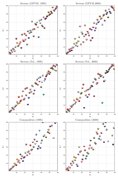
After tracing the probabilities $P(K),P^{*}(K^{*})$ over sectors we obtain the distribution of world countries on the PageRank-CheiRank plane $(K_{c},K^{*}_{c})$ presented in Fig. 4 for WNEA in years 1995, 2008. In the same figure we present the rank distributions obtained from ImportRank-ExportRank probabilities of exchange value and the results obtained in wtngoogle for the WTN with all commodities. For the GPVM data we see the global features already discussed in wtngoogle : the countries are distributed in a vicinity of diagonal $K_{c}=K^{*}_{c}$ since for each country the size of imports is correlated with the size of exports, even if trade is never exactly balanced and some countries can sustain significant trade surplus or deficit. The top $20$ list of top $K_{2}$ countries recover $13$ of 19 countries of $G20$ major world economies (EU is the number 20) thus obtaining 68% of the whole list. This is close to the percent obtained in wtngoogle for trade in all commodities. The Google ranking for WNEA and WTN (top and bottom panels in Fig. 4) gives different positions for specific countries (e.g. Russia improves its position for WNEA with the opposite trend for China) but the global features of distributions of WNEA and WTN remain similar corresponding to the same economical forces.

Figure 5: Two dimensional ranking of sectors on the ($K_{s}$,$K^{*}_{s}$) plane using the GPVM approach for PageRank and CheiRank (left panels) and ImportRank-ExportRank (right panels). Each sector is represented by its specific combination of color and symbol. The list of all $37$ sectors are given in Table 2. Top panels show the case for the year 1995 and bottom panels for the year 2008.

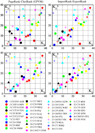
After tracing over countries we obtain the PageRank-CheiRank plane of activity sectors shown in Fig. 5. We see that some sectors are export oriented (e.g. $s=2$ C10T14 Mining at $K_{s}^{*}=1$ in 2008) others are import oriented (e.g. $s=23$ C50T52 World Retail and Trade of motors etc. at $K_{s}=1$ in 2008). The ImportRanking gives a rather different import leader $s=7$ C23 Manufacture of coke, refined petroleum products etc. with $K_{s}=1$ in 2008. Thus the Google ranking highlights highly connected network nodes while Import-Export gives preference to high value neglecting existing network relations between various countries and activity sectors. We can also order sectors by 2DRank index $K_{2}$ getting for PageRank-CheiRank top sectors $s=25,23,8$ at $K_{2}=1,2,3$ while Import-Export gives $s=8,11,14$ for top $K_{2}$ values in 2008 (more data are given at ourwebpage ). We note that $s=25$ corresponds to Transport which has many network connections thus taking the top $K_{2}$ position. We note that asymmetry of ranking of products has been discussed in wtnproducts for COMTRADE data, however, the comparison with these data is not so simple since the correspondence between products and activity sectors is not straightforward. Of course, for the WNEA the asymmetry of sector ranking exists even for Export-Import ranking, in a drastic difference from the WTN, since there are interactions between activity sectors.

The global ranks of top 20 countries and their activities are given in Table 4 for 2008. The top 3 places of PageRank $K=1,2,3$ are taken by Germany (Manufacture of motors etc. $s=18$), USA (Public administration and defence $s=33$), ROW (also $s=33$). Thus imports of arms and weapons play a very important role. In contrast for ImportRank $\hat{K}=1,2,3$ we find rather different results with USA (petroleum $s=7$), Japan (also $s=7$), and only then USA ($s=33$). For CheiRank $K^{*}=1,2,3$ we find ROW, Russia, Saudi Arabia ($s=2$ C10T14 Mining) while for ExportRank we have ROW, Saudi Arabia, Russia ($s=2$ C10T14 Mining) respectively. Thus Russia goes ahead of Saudi Arabia due to a broad network of activity and trade connections (a similar effect has been found in wtngoogle ; wtnproducts for trade in petroleum). The top 3 positions of 2DRank $K_{2}=1,2,3$ are taken by Germany ($s=8$ Manufacture of chemicals etc.). USA ($s=27$ Finance etc.), Germany ($s=13$ Manufacture of machinery etc.).

Figure 6: Left column panels show results of the GPVM data for country positions on PageRank-CheiRank plane of local rank values $K_{c},{K_{c}}^{*}$ ordered by ($K_{cs},{K^{*}}_{cs}$) for specific sectors with $s=21$ (top), $s=28$ (center) and $s=1$ (bottom). Right column panels show the ImportRank-ExportRank planes respectively for comparison. Data are given for year 2008. Each country is shown by its own flag as in Fig 4.

Figure 7: Global plane of rank indexes ($K,K^{*}$) for PageRank-CheiRank (left panel) and ImportRank-ExportRank (right panel) for $N=2146$ nodes in year 2008. Each country and sector pair is represented by a gray square. Some countries are highlighted in colors : USA in black, South Korea in red, China (and Taiwan) in green, Russia in blue, France in yellow and Brazil in orange.

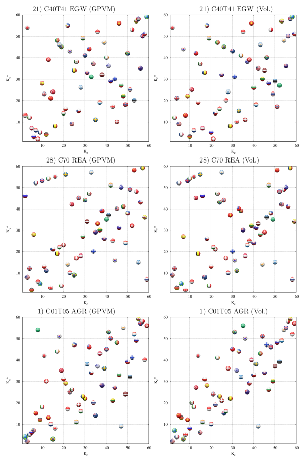
We can fix a certain activity sector $s$ and then consider local ranking of countries in $(K_{c},{K_{c}}^{*})$ plane. Three examples are shown in Fig. 6 for $s=21$ (Electricity, gas, water), $28$ (Real estate activity), $1$ (Agriculture). The comparison of Google ranking (left column) with value Import-Export ranking (right column) shows importance of network connections highlighted by the GPVM, thus Russia moves from ${K_{c}}^{*}=4$ on right panel to $K_{c}^{*}=2$ on left panel for $s=21$ due to its broad links with Europe and Asia. For $s=1$ case in bottom panels of Fig. 6 we find that the Import-Export ranking distribution is more clse to diagonal comparing to the PageRank-CheiRank case that we attribute to effect of indirect links present in the later case.

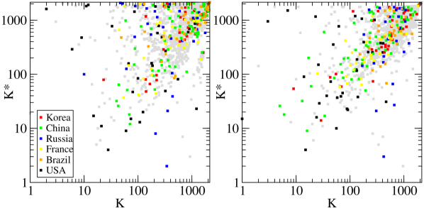
The distribution of nodes on the global $(K,K^{*})$ plane is shown in Fig. 7 for Google ranking (left panel) and Import-Export ranking (right panel) in 2008. The majority of countries are shown by gray squares while 6 selected countries are marked by colors. The comparison of two panels show that in the Google ranking the positions of USA are improved (more black symbols at top $K_{2}$ positions) while for China the positions (green symbols) are weakened. We attribute this to a broader network connections of USA in important activity sectors world wide (e.g. military activities and defense).

3.3 Correlation properties of PageRank and CheiRank

The directed networks can be characterized by the correlator $\kappa$ of PageRank and CheiRank vectors. For various networks the properties of $\kappa$ are reported in linux ; arxivrmp . There are directed networks with small or even slightly negative values of $\kappa$, e.g. Linux Kernel or Physical Review citation networks, or with $\kappa\sim 4$ for Wikipedia networks and even larger values $\kappa\approx 116$ for the Twitter network.

Figure 8: PageRank-CheiRank correlators $\kappa_{s}$ from the GPVM (see (15), (16)) are shown as a function of the sector index $s$ with the corresponding symbol from Fig.5. PageRank-CheiRank and ImportRank-ExportRank correlators are shown by solid and dashed lines respectively, where the global correlator $\kappa$ (14) is shown in black, the correlator for countries $\kappa(c)$ (17) is shown by red lines, the correlators for sectors $\kappa(s)$ (17) is shown by blue lines. Here sector index $s$ is counted in order of appearance in Table 2. The data are given for year 2008 with $N_{s}=37$, $N_{c}=58$, $N=2146$.

The correlators of WNEA for various sectors are shown in Fig. 7. Almost all correlators $\kappa_{s}$ are positive being distributed in a range $(0,1)$. A small negative value appears only for $s=37$ (Private households etc.) corresponding to anti-correlation between buyers and sellers. The largest correlator $\kappa_{s}$ is for $s=29$ (Renting of machinery etc.) shows that sales of machinery correlates with their purchases probably because components are needed to produce machines produced by firms in the same industrial sectors.

The matrix of correlators between sectors $s,s^{\prime}$ is shown in Fig. 8 for years 1995, 2008. It is interesting to see a significant shift of line of maximal correlators located in 1995 at $s^{\prime}=28$ (Real estate activities) to $s=29$ (Renting of machinery etc.) in 2008. We also see that there are less correlations between sectors in 2008 compared to 1995. A further more detailed analysis of correlations would bring a better understanding of hidden inter-relations between various sectors of economic activity.

Figure 9: Top panels: Spectrum of Google matrices $G$ (left) and $G^{*}$ (right) represented in the complex plane of $\lambda$. The data are for year 2008 with $\alpha=1$, $N=2146$, $N_{c}=58$, $N_{s}=37$. Four eigenvalues marked by colored circles are used for illustration of eigenstates in Fig. 10 and Table 5. Bottom panels: Inverse participation ratio (IPR) $\xi$ of all eigenstates of $G$ (left) and $G^{*}$ (right) as a function of the real part of the corresponding eigenvalue $\lambda$ from the spectrum above.

3.4 Spectrum and eigenstates of WNEA Google matrix

The results obtained for the Wikipedia network wikispectrum and the multiproduct WTN wtnproducts demonstrated that the eigenvectors of $G$ and $G^{*}$ with large eigenvalue modulus $|\lambda|$ select certain specific communities. Thus it is interesting to analyze the properties of eigenvalues for the WNEA. At $\alpha=1$ the gap between $\lambda=1$ and other eigenvalues characterize the rate of system relaxation to the equilibrium stationary PageRank state (for $G$). The presence of small gap indicates that the mixing and relaxation in the system are developed only after many iterations of $G$ matrix (see more discussion in arxivrmp ).

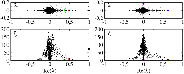
The matrix size of WNEA is relatively small and the whole spectrum $\lambda$ of $G,G^{*}$ can be determined by direct matrix diagonalization. The spectrum is shown in top panels of Fig. 9. It is characterized by a significant gap between $\lambda=1$ and other eigenvalues with $|\lambda|<0.7$ at $\alpha=1$. We attribute this to a large number of inter-connected links between matrix nodes (countries and sectors) which is usually responsible for appearance of the spectral gap (see physrev , where the gap increases with the increase of number of random links per node). We also note that the maximal value of $|\mathit{Im}\lambda|<0.2$ is relatively small due to presence of links going in direct and inverse directions between nodes. These features show that the relaxation processes to the steady-state PageRank vector are relatively rapid on the WNEA. Indeed, the relaxation is governed by the exponent $\exp(-\Delta\lambda t)$ where $\Delta\lambda\approx 0.25$ the gap for for WNEA in Fig. 9 and $t$ is number of iterations of $G$.

Figure 10: Eigenstates amplitudes $|\psi_{i}|$ ordered by its own decreasing amplitude order with local rank index $K_{i}$ for 4 different eigenvalues of Fig. 9 (states are normalized as $\sum_{i}|\psi_{i}|=1$). The four examples are $\lambda=0.4993$ (red), $\lambda=0.3746+0.0126i$ (green), $\lambda=0.6256$ (blue) and $\lambda=-0.0001+0.1687i$ (magenta). Node names (country, sector) for top ten largest amplitudes of these eigenvectors are shown in Table 5.

The properties of eigenstates are characterized by the IPR $\xi$ shown in bottom panels of Fig. 9. We find that the main part of states have $\xi\ll N$ so that they occupy only a small fraction of nodes corresponding to localized states (see discussion about the Anderson localization of Google matrix eigenstates in arxivrmp ; zsanderson ).

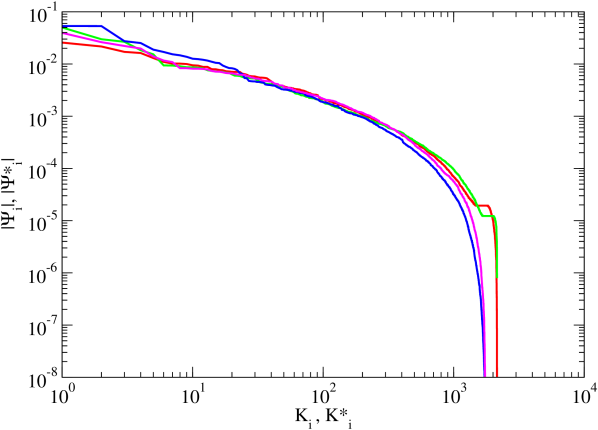
The dependence of amplitudes $|\psi_{i}|$ of a few eigenstates, ordered by a local rank index $K_{i}$ corresponding to a monotonic amplitude decrease, are shown in Fig. 10. The names of top 10 nodes of these eigenstates are given in Table 5. The red curve in Fig. 10 selects mainly the sector $s=4$ (Manufacture of textiles etc.) with close links between China, Italy, USA and ROW; the green one selects $s=18$ (Manufacture of motor vehicles etc.) with close links between Argentina, Brasil, Japan and Germany; the blue state corresponds to $s=16$ (Manufacture of radio, television and communication equipment and apparatus) in the Asian region (China, Korea, Chinese Taipei, Singapore, Malaysia); the magenta state represents sector $s=2$ (Mining etc.) with related countries like Russia, Saudi Arabia, ROW, Norway. These results coincide with the previous observations for Wikipedia-type network wikispectrum that the eigenstates of $G$ and $G^{*}$ select specific communities of the network nodes. Similar properties of eigenstates of $G$ of the multiproduct WTN have been found in wtnproducts .

3.5 Sensitivity to price variations

The ranking of WNEA nodes provides interesting and important information. In addition, the established matrix structure of $G,G^{*}$ of WNEA also allows to study the sensitivity of the world economic activities to price variations. There are certain parallels with the multiproduct WTN analyzed in wtnproducts but there are also new elements specific to the WNEA.

Figure 11: Left panel: Derivatives $D=dP/d\delta_{7}$ and $D^{*}=dP^{*}/d\delta_{7}$ for a price variation $\delta_{7}$ of 7 C23 PET (Manufacture of coke, refined petroleum products and nuclear fuel) for year 2008. Right panel: Logarithmic derivatives $D_{l}=D/P$ and $D^{*}_{l}=D^{*}/P^{*}$ for the same case as left panel. Codes in panels give sector number $s=1,...37$ described in Table 2, country codes are from Table 1. The group of points, highlighted by the dashed box, represents $58$ nodes of the form $(country,s=7)$ where $s=7$ is C23 PET (Manufacture of coke, refined petroleum products and nuclear fuel).

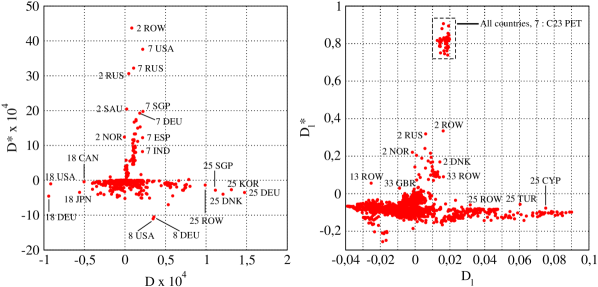
To analyze the sensitivity of price variation in a certain activity sector $s$ we increase from $1$ to $1+\delta_{s}$ the money transfer in the sector $s$ in $M_{cc\,ss^{\prime}}$ in (1), where $\delta_{s}$ is a dimensionless fraction variation of price in this sector. After that the matrices $G,G^{*}$ are recomputed in the usual way described above and their rank probabilities $P,P^{*}$ are determined. Then we compute the derivatives of probabilities of PageRank $D=dP/d\delta_{s}=\Delta P/\delta_{s}$ and CheiRank $D^{*}=dP^{*}/d\delta_{s}=\Delta P^{*}/\delta_{s}$. We do these computations at sufficiently small $\delta_{s}$ values checking that the variations of $P,P^{*}$ are linear in $\delta_{s}$. In addition we also compute the logarithmic derivatives $D_{l}=d\ln P/d\delta_{s}$, $D^{*}_{l}=d\ln P^{*}/d\delta_{s}$ which give us relative changes of $P$, $P^{*}$.

The sensitivities to price of $s=7$ (Manufacture of coke, refined petroleum products and nuclear fuel) are shown in Fig. 11. The data for $D,D^{*}$ in the left panel show a rather complex picture with a significant derivatives not only for $s=7$ but also for countries with sectors: $s=18$ (Manufacture of motor vehicles, trailers and semi-trailers) at strongly negative $D$ for Germany. USA, Japan; $s=25$ (Land transport; transport via pipelines etc) at significant positive $D$ for Germany. Korea, Denmark, Singapore; of course, for $s=7$ we have positive $D^{*}$, but also for $s=2$ related to mining and negative $D^{*}$ for $s=8$ (Manufacture of chemicals and chemical products) for USA and Germany. The logarithmic derivatives provide strong relative changes and are shown in the right panel of Fig. 11.

Figure 12: Same as the left panel of Fig. 11 but using probabilities from the trade value. In the right panel, $D^{*}_{l}=0.9348$ if $s=s^{\prime}$ and $D^{*}_{l}=-0.0633$ if $s\neq s^{\prime}$.

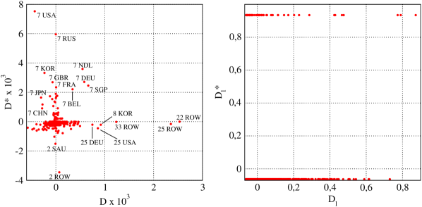
A similar analysis can be done using the probabilities $\hat{P},\hat{P}^{*}$ from the exchange value probabilities (3) instead of the above PageRank and CheiRank probabilities. The results for the value probabilities are presented in Fig. 12 for the same case as in Fig. 11. We see that the results are drastically different especially for the logarithmic derivatives $D_{l},D^{*}_{l}$. In fact $D_{l},D^{*}_{l}$ cannot give correct picture of sensitivity to price variations since for the monetary exchange the network links between nodes are not taken into account and there is only a mechanical re-computation of the value normalization. A similar situation appears also for the multiproduct WTN wtnproducts . Thus we see from Fig. 11 and Fig. 12 that the Google matrix approach provides new elements for the economic activity analysis going significantly beyond the usual consideration of Import-Export method.

The new element of the WNEA, compared to the multiproduct WTN, is existence of transfers between sectors of the same economy. This allows us to consider the sensitivity not only to sectoral prices but also the sensitivity to labor cost in a given country $c$ (e.g. price shock affecting all industries in the same country). This can be taken into account by the introduction of the dimensionless labor cost change in a given country $c$ by replacing the related monetary flows from coefficient $1$ to $1+\sigma_{c}$ in $M_{cc^{\prime},ss;}$ (1) for a selected country $c$.

Of course, the above derivatives over price of activity sector and labor country cost give only an approximate consideration of effects of price variations which is a very complex phenomenon. For an economic discussion of the effect of price shocks on international production networks we address a reader to the research performed in escaith . We will see below that our approach gives results being in a good agreement with economic realities thus opening complementary possibilities of economic activity analysis based on the underlying network relations between countries and activity sectors which are absent in the usual Import-Export consideration. We present the results on sensitivity to sector prices and labor cost in next subsections.

3.6 Price shocks and trade balance sensitivity

On the basis of the obtained WNEA Google matrix we can now analyze the trade balance in various activity sectors for all world countries. Usually economists consider the export and import of a given country as it is shown in Fig. 1. Then the trade balance of a given country $c$ can be defined making summation over all sectors:

$$B_{c}=\sum_{s}(P^{*}_{cs}-P_{cs})/\sum_{s}(P^{*}_{cs}+P_{cs})=(P^{*}_{c}-P_{c})/(P^{*}_{c}+P_{c}).$$ (18)

In economy, $P_{c},P^{*}_{c}$ are defined via the probabilities of trade value $\hat{P}_{cs},\hat{P}^{*}_{cs}$ from (3). In our matrix approach, we define $P_{cs},P^{*}_{cs}$ as PageRank and CheiRank probabilities. In contrast to the Import-Export value our approach takes into account the multiple network links between nodes.

Figure 13: World map of CheiRank-PageRank balance $B_{c}=(P^{*}_{c}-P_{c})/(P^{*}_{c}+P_{c})$ determined for all ${N_{c}}=58$ countries in year 2008. Top panel shows the probabilities $P$ and $P^{*}$ given by PageRank and CheiRank vectors; the value of ROW group is $B_{c=58}=0.023$. Bottom panel shows the probabilities $P$ and $P^{*}$ computed from the Export and Import value; the value of ROW group is $B_{c=58}=0.16$. Names of the countries are given in Table 1 and in the world map of countries worldmap .

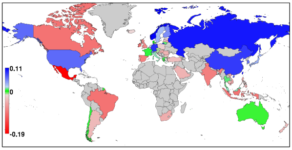
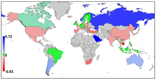
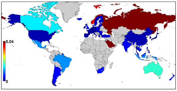
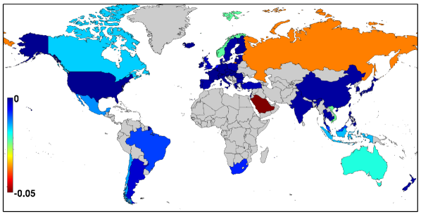
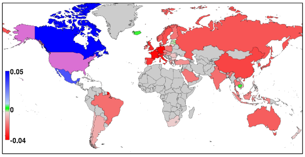
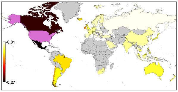
The comparison of CheiRank-PageRank balance with Export-Import balance for the world countries shown in Fig. 13 for year 2008. Each country is shown by color whcih is proportional to the country balance $B_{C}$ (18) with the color bar given on the figure. For Export-Import balance we see the dominance of petroleum producing countries Saudi Arabia, Russia, Norway with the largest values. The      CheiRank-PageRank balance highlights new features placing on the top Russia, Norway, Germany, China. In fact, USA has now a slightly positive balance in top panel of Fig. 13) while it was negative before in bottom panel of same figure. We see that the broad network of economic activity relations and links makes the economies of the above countries more important in the world economy while Saudi Arabia, with the largest positive Export-Import balance, looses its leading position. Indeed, the trade of this country is mainly oriented to USA and nearby countries that reduces its importance for world economy (a similar effect has been observed with COMTRADE data wtngoogle ; wtnproducts ).

Figure 14: Derivative of probabilities balance $dB_{c}/d\delta_{7}$ over price of sector $s=7$ C23PET for year 2008. Top panel shows the case when $B_{c}$ is determined by CheiRank and PageRank vectors as in the top panel of Fig.13; the value of ROW group is $dB_{58}/d\delta_{7}=0.04$. Bottom panel shows the case when $B_{c}$ is computed from the Export-Import value as in the bottom panel of Fig.13; the value of ROW group is $dB_{58}/d\delta_{7}=-0.07$. Names of the countries can be found in Table 1 and in the world map of countries worldmap .

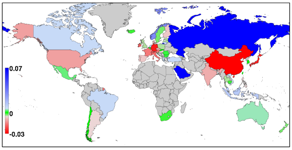
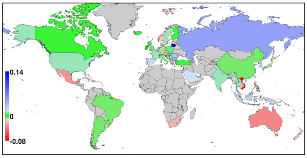
The sensitivity of country balance $dB_{c}/d\delta_{7}$ to price variation of sector $s=7$ Manufacture of coke, refined petroleum products and nuclear fuel is shown in Fig. 14. For Export-Import in bottom panel the most sensitive countries are Lithuania (positive) and Vietnam (negative). Lithuania does not produce petroleum, but in fact in 2008 there was a large oil refinery company there which had a large exportation value (see e.g.
http://en.wikipedia.org/wiki/Economy_of_Lithuania). The Export-Import approach shows that Russia is slightly positive, even less positive is Saudi Arabia, China and Germany are close to zero change, USA is only very slightly positive. The results of CheiRank-PageRank sensitivity (top panel) are significantly different showing strongly positive sensitivity for Saudi Arabia, Russia and strongly negative sensitivity for China, Germany and Japan; USA goes from slightly positive side in bottom panel to moderate negative one in top panel. The CheiRank-PageRank balance demonstrates much higher sensitivity of Russia, Saudi Arabia and China to price variations of $s=7$ sector comparing to the case of Export-Import value analysis. The economies of Germany, China and Japan are also very sensitive to petroleum prices that is correctly captured by our analysis. We consider that the CheiRank-PageRank approach describes the economic reality from a new complementary angle and that provides new useful information about complex trade systems. We also note that the highly negative sensitivity of China to     petroleum prices has been also obtained on the basis of Google matrix analysis of COMTRADE data (see Fig.21 in wtnproducts ).

Figure 15: Derivative of partial probability balance of sector $s$ defined as $dB_{cs}/d\delta_{s^{\prime}}$ over sector $s^{\prime}=7$ C23PET price $\delta_{7}$ for year 2008. Here $B_{cs}=(P^{*}_{cs}-P_{cs})/(P^{*}_{c}+P_{c})$ and $s=2$ (C10T14MIN, Mining, extraction,…) from Table 2. The sector balance sensitivity of countries $B_{cs}$ is determined from CheiRank and PageRank vectors (top panel) and from the exchange value of Export-Import (bottom panel); the values of ROW group are $dB_{58,2}/d\delta_{7}=0.05$ and $dB_{58,2}/d\delta_{7}=-0.03$ respectively. Names of the countries can be found at Table 1 and in the world map of countries worldmap .

It is also possible to determine the cross-sensitivity of activity sectors to price variation. For that we determine the partial exchange balance for a given sector $s$ defined as

$$B_{cs}=(P^{*}_{cs}-P_{cs})/\sum_{s}(P^{*}_{cs}+P_{cs})=(P^{*}_{cs}-P_{cs})/(P^{*}_{c}+P_{c}),$$ (19)

so that the global country balance is $B_{c}=\sum_{s}B_{cs}$. Then the sensitivity of partial balance of a given sector $s$ in respect to a price variation of a sector $s^{\prime}$ is given by the derivative $dB_{cs}/d\delta_{s^{\prime}}$. The results for $s=2,s^{\prime}=7$ are shown in Fig. 15. We see that two methods give results with even opposite signs. According to the Google matrix analysis the increase of petroleum prices stimulates development of mining while for the Export-Import approach the result is the opposite. In our opinion, the absence of links and next step relations between countries and sectors in the Export-Import methods does not allow to take into account all complexity of economy relations. In contrast the CheiRank-PageRank approach captures effects of all links providing more advanced indications.

Figure 16: Top (China) and bottom (USA) panels show derivative $dB_{c}/d\delta_{s^{\prime}}$ of country total probability balance $B_{c}$ over price $\delta_{s^{\prime}}$ of sector $s^{\prime}$ for year 2008 (black points connected by dashed line); derivatives of balance without diagonal term ($dB_{c}/d\delta_{s^{\prime}}-dB_{cs^{\prime}}/d\delta_{s^{\prime}}$) are represented by open red circles. The sector balance of countries $B_{cs}$ and $B_{c}$ are determined from CheiRank and PageRank vectors. The sectors corresponding to sector index $s$ or $s^{\prime}$ are listed in Table2.

Figure 17: China (top) and USA (bottom) examples of derivative $dB_{cs}/d\delta_{s^{\prime}}$ of partial probability balance $B_{cs}$ of sector $s$ over price $\delta_{s^{\prime}}$ of sector $s^{\prime}$ for year 2008. Diagonal terms, given by $y=dB_{cs}/d\delta_{s}$ for $s=s^{\prime}$, are shown on the top panels of each example. Sectors $s^{\prime}$ and $s$ are shown in $x$-axis and $y$-axis respectively (indexed as in Table2 from $1$ to $37$), while $dB_{cs}/d\delta_{s^{\prime}}$ is represented by colors with a threshold value given by $+\epsilon$ and $-\epsilon$ for negative and positive values respectively, also shown in red dashed lines on top panels with diagonal terms. Here $\epsilon=0.01$ for USA and China; partial balance $B_{cs}$ is defined by CheiRank and PageRank probabilities.

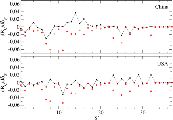
The sensitivities $dB_{c}/d\delta_{s^{\prime}}$ of CheiRank-PageRank balance of China and USA to price variation of sectors $s^{\prime}$ are presented in Fig. 16. We see two rather different profiles. Thus, for China the derivative $dB_{c}/d\delta_{s^{\prime}}$ is positive for sectors $s=4,14,16$ (Manufacture of textiles; office machinery; radio etc,) and negative for $s=7,25,27$ (Petroleum; Land transport etc.; Financial intermediation etc.). For USA the sensitivity is significantly positive for $s=23,29,32$ (Sale of motor vehicles etc.; Renting of machinery and equipment etc.; Other business activities) and negative for $s=11$ (Manufacture of basic metals). Thus the economic activities of these two countries have very different strong and weak points. We note that the sensitivity without the diagonal term ($dB_{c}/d\delta_{s^{\prime}}-dB_{cs^{\prime}}/d\delta_{s^{\prime}}$) has negative values for almost all sectors for both countries.

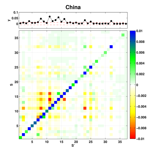
The matrices of cross-sector sensitivity $dB_{cs}/d\delta s^{\prime}$ are shown for China and USA in Fig. 17. Such matrices provide a detailed information of interconnections of various activity sectors. Thus for USA we see that its $s=8$ (Manufacture of chemicals etc.) has a significant negative sensitivity to $s^{\prime}=7,23,25$ (Petroleum; Renting of machinery and equipment etc.; Land transport etc.). Indeed, chemical production is linked with petroleum, machinery and transport. For China we find that its sector $s=11$ (Manufacture of basic metals) has a negative sensitivity to $s^{\prime}=8,23$ (Manufacture of chemicals etc.; Renting of machinery and equipment etc.); also $s=14,16$ have a negative derivative in respect to $s^{\prime}=11$).

Of course, the cross sensitivity to price variations in one sector and their effects on another sector, based on (19), is a very delicate thing since a price in one sector can affect prices in other sectors also in other manner since economic systems learn and adapt while here we considered only linear algebraic relations without any adaptation features. However, even being linear, the Google matrix approach provides a detailed information on hidden interactions and inter-dependencies of various economic activities for various countries that can provide a useful message even for nonlinear adapting systems.

Figure 18: Derivative of probabilities balance $dB_{c}/d\sigma_{c^{\prime}}$ over labor cost of China $c^{\prime}=37$ for year 2008. Top panel shows the case when $B_{c}$ is determined by CheiRank and PageRank vectors; here the special values are $dB_{58}/d\sigma_{37}=-0.0146$ for ROW group (gray) and $dB_{37}/d\sigma_{37}=0.3217$ for China (magenta). Bottom panel shows the case when $B_{c}$ is computed from the Export-Import value; the special values are $dB_{58}/d\sigma_{37}=-0.0352$ for ROW group (gray) and $dB_{37}/d\sigma_{37}=0.4810$ for China (magenta). Names of the countries can be found in Table 1 and in the world map of countries worldmap .

3.7 World map of sensitivity to labor cost

Using the established structure of WNEA we can study the sensitivity of country balance $dB_{c}/d\sigma_{c}^{\prime}$ to the labor cost in different countries. At the difference of sectoral shocks on one product, here the price shock affects all industries in a country. As before, the change in price has to be small enough for the resulting simulation to remain in a neighbourhood of the original data. Indeed, larger shocks would trigger a series of substitution effects diverting trade to other partners.

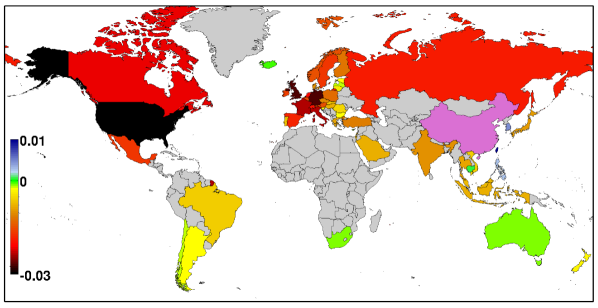
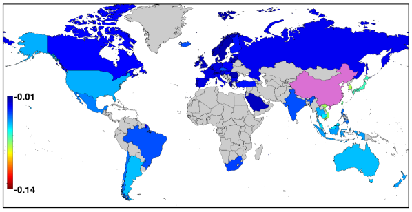
The derivative $dB_{c}/d\sigma_{c}^{\prime}$ is computed numerically as described in Sec. 3.5. The world sensitivity to the labor cost of China is shown in Fig. 18. Of course, the largest derivative is found for China itself ($dB_{c}/d\sigma_{c}$ at $c=37$ from Table 1). The effect on other countries is given by non-diagonal derivatives at $c\neq c^{\prime}=37$. From the CheiRank-PageRank balance we find that the most strong negative effect (minimal negative $dB_{c}/d\sigma_{c^{\prime}}$) is obtained for USA, Germany, UK; a positive derivative is visible only for Chinese Taipei ($s=38$) and S.Korea ($s=19$). For the Export-Import balance the results are rather different: at first all derivatives at $c\neq c^{\prime}$ are negative; among the most negative values are such countries as Hong Kong (most negative with dark red color but hardly visible due to its small size), Chinese Taipei, S.Korea, Vietnam. Thus the Google matrix approach bring a new perspective for analysis of complex of economical relations between countries and sectors.

Figure 19: Same as in Fig. 18 with the derivative $dB_{c}/d\sigma_{c^{\prime}}$ over the labor cost $c^{\prime}=11$ of Germany for year 2008. Top panel shows the case when $B_{c}$ is determined by CheiRank and PageRank vectors; the special values are $dB_{58}/d\sigma_{11}=-0.0367$ for ROW group (gray) and $dB_{11}/d\sigma_{11}=0.3248$ for Germany (magenta). Bottom panel shows the case when $B_{c}$ is computed from the Export-Import value; the special values are $dB_{58}/d\sigma_{11}=-0.0280$ fro ROW group (gray) and $dB_{11}/d\sigma_{11}=0.4911$ for Germany (magenta). Names of the countries can be found in Table 1 and in the world map of countries worldmap .

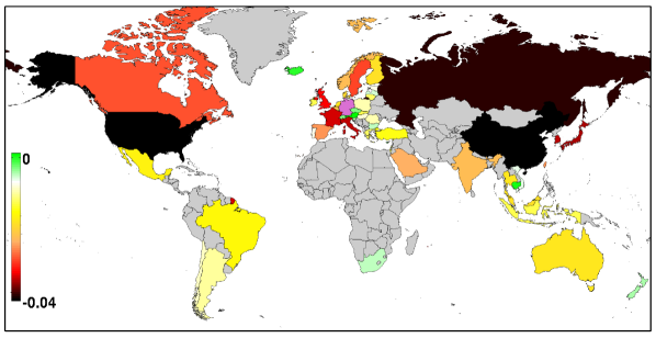
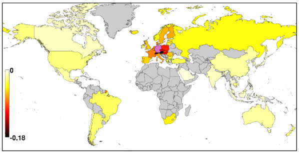
Another results for the effects of labor cost in Germany and in USA are shown in Fig. 19 and Fig. 20. In the case of Germany the most strong negative sensitivity is for USA, Russia, China for CheiRank-PageRank balance while for Import-Export it is Switzerland and Austria. However, USA and Russia are relatively weakly affected. This again stresses the qualitative difference between these two approaches.

The increase of USA labor cost in Fig. 20 produces positive derivatives of CheiRank-PageRank balance for Canada and Mexico that looks reasonable from a view point of economy since these countries will profit from higher production costs in USA. In opposite, Export-Import gives most strong negative derivatives for Canada and Mexico.

Figure 20: Same as in Fig. 18 with the derivative $dB_{c}/d\sigma_{c^{\prime}}$ over labor cost $c^{\prime}=34$ of USA for year 2008. Top panel shows the case when $B_{c}$ is determined by CheiRank and PageRank vectors; the special values are $dB_{58}/d\sigma_{34}=-0.0257$ for ROW group (gray) and $dB_{34}/d\sigma_{34}=0.3148$ for USA (magenta). Bottom panel shows the case when $B_{c}$ is computed from the Export-Import value; the special values are $dB_{58}/d\sigma_{34}=-0.0632$ for ROW group (gray) and $dB_{34}/d\sigma_{34}=0.4852$ for USA (magenta). Names of the countries can be found in Table 1 and in the world map of countries worldmap .

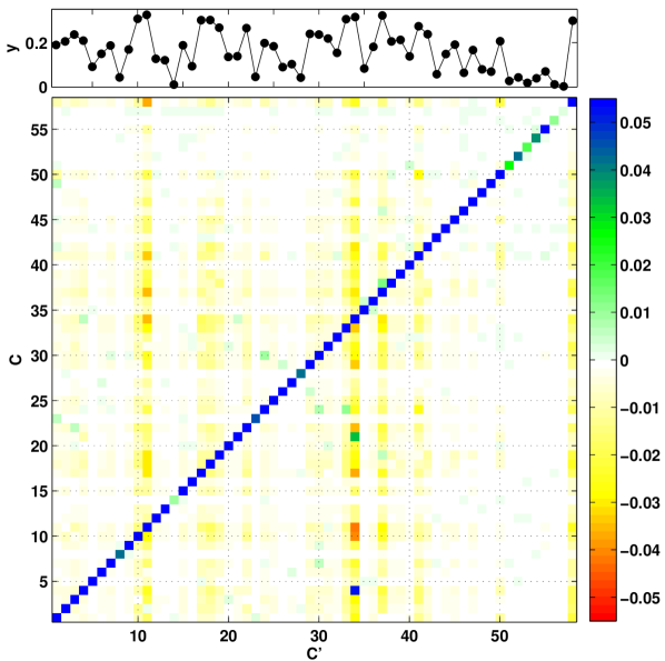
The whole matrix of labor cost derivatives $dB_{c}/d\sigma_{c^{\prime}}$ of the CheiRank-PageRank balance $B_{c}$ is shown in Fig. 21 (numerical values of derivatives are given at ourwebpage ). Of course, the diagonal terms have the strongest positive derivatives, but off-diagonal terms change signs and characterize the sensitivity of one country to labor cost in other country. The vertical lines with high derivative values correspond to Germany ($c^{\prime}=11$), Japan ($c^{\prime}=18$), S.Korea ($c^{\prime}=19$), USA ($c^{\prime}=34)$, China ($c^{\prime}=37$), Russia ($c^{\prime}=41$). The rest of the world (ROW) group also have a visible effect of other countries ($c^{\prime}=58$). Thus is it desirable to obtain individual OECD data for countries of the ROW group.

Figure 21: Global view of the effect of labor cost variation in country $c^{\prime}$ on country $c$ in 2008. Matrix elements $dB_{c}/d\sigma_{c^{\prime}}$ are given in colors shown by the truncated color scale; matrix elements above the scale (diagonal terms) are shown in the top inset where $y=dB_{c}/d\sigma_{c^{\prime}}$. In the matrix of derivatives shown by color, $x$-axis shows the index $c^{\prime}$ of country where a labor cost variation $\sigma_{c^{\prime}}$ takes place and $y$-axis shows the country $c$ affected by the change. Here $B_{c}$ is computed from CheiRank and PageRank probabilities. Country identification numbers $c=1,...,58$ are given in Table 1.

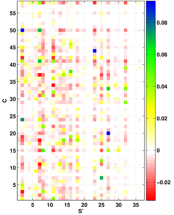
In Fig. 21 we considered the effects of the labor cost in various countries. We can also see the effect of price variation $\delta_{s^{\prime}}$ in a given sector $s^{\prime}$ on the CheiRank-PageRank balance $B_{c}$ of country $c$. This sensitivity is given by the rectangular matrix of derivatives $dB_{c}/d\delta_{s^{\prime}}$ shown in Fig. 22 (numerical data are given at ourwebpage ). The strongest positive derivatives (blue squares) are for $s^{\prime}=2,c=50$ (mining and Saudi Arabia), $s^{\prime}=23,c=44$ (motors and Hong Kong), $s^{\prime}=27,c=20$ (finance and Luxembourg). The strongest negative derivatives (red squares) are for $s^{\prime}=2,c=3$ (mining and Belgium), $s^{\prime}=2,c=42$ (mining and Singapore which economy is very sensitive to mining products), $s^{\prime}=7,c=11$ (petroleum and Germany), $s^{\prime}=7,c=18$ (petroleum and Japan), $s^{\prime}=7,c=37$ (petroleum and China), $s^{\prime}=11,c=34$ (manufacture of basic metals and USA), $s^{\prime}=11,c=42$ (manufacture of basic metals and Singapore). All these results are in agreement with the economic realities of sensitivity of the above countries to given activity sectors. This shows the strength of the Google matrix approach to analysis of WNEA.

Figure 22: Global view of the effect of sector $s^{\prime}$ price variation on balance of country $c$ in 2008. Colors are proportional to matrix elements $dB_{c}/d\delta_{s^{\prime}}$, $x$-axis shows the sector index $s^{\prime}$ (sectors are given in Table 2) and $y$-axis gives the country index $c$ affected by the change (countries are given in Table 1). Here $B_{c}$ is computed from CheiRank and PageRank probabilities.

3.8 World transformation matrix of activity sectors

From the obtained Google matrices $G,G^{*}$ of WNEA we can analyze the transformation of the activity sectors by the world economy. For this analysis we compute the transfer matrix

$$T=(1-\eta)(1-\eta G^{*})^{-1}G\;\;,$$ (20)

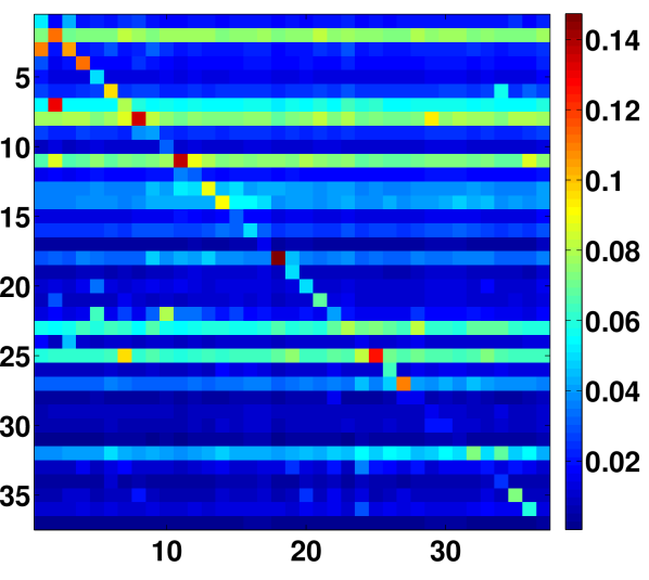
where $\eta$ is a numerical constant. Our study show that as in the case of damping factor $\alpha$ the results are robust to variations of $\eta$ in the range $0.5<\eta<0.9$ and thus in the following we present the results for $\eta=0.7$. We note that a similar construction for ImpactRank has been used for Wikipedia networks physrev and the C.elegans neural network celegans . In a certain sense (20) can be considered as a scattering matrix of particles entering in a system by $G$ term and then going out by the expansion term $1+\eta G^{*}+(\eta G^{*})^{2}....=1/(1-\eta G^{*})$. In this approach $\eta$ describes a relaxation rate in the system. We note that $T$ belongs to the Google matrix class.

From the global matrix $T$ of size $N$ we obtain the reduced matrix $R_{ss^{\prime}}(c)$ of size $N_{s}$ describing the transformation for activity sectors for a country $c$. We have $R_{ss^{\prime}}(c^{\prime})=\sum_{c}T_{s,s^{\prime},c,c^{\prime}}$ where $c^{\prime}$ is a target country we are interested in. The matrices $R_{ss^{\prime}}(c^{\prime})$ giving the transformation of sector $s^{\prime}$ to all other sectors $s$ for $c^{\prime}$ of China, USA, Germany are given in ourwebpage . The reduced transformation matrix for the whole world is obtained by averaging over countries with $R_{ss^{\prime}}=\sum_{c^{\prime}}R_{ss^{\prime}}(c^{\prime})/N_{c^{\prime}}$ (see Fig. 23). The results of Fig. 23 show a few characteristic features: the reduced transfer matrix has a strong diagonal element (this is because each product is strong projection on itself), there are characteristic horizontal lines corresponding to important sectors (e.g. $s=2,7,11,25$).

Figure 23: Image of the average reduced transfer matrix $R_{s,s^{\prime}}$ of sectors to sectors for for the whole world (averaged over countries) for year 2008. Here $x$-axis represents the initial sector $s^{\prime}$ and $y$-axis represents the final sectors $s$ into which $s^{\prime}$ is transformed. The sector numbering is given in Table 2. Colors are proportional to matrix elements and $\eta=0.7$.

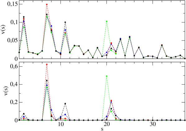
By considering a transformation of a given sector to all other sectors for a given country. For $s^{\prime}=2$ (mining) we present the resulting transformed vector $v(s)$ in Fig. 24 for France, Germany, Switzerland and USA. The global profiles are similar but there are significant enhancement for Germany at sector $s=7$ (petroleum) and for Switzerland at sector $s=20$ (manufacturing and recycling). For comparison we show the results of transformation of input/output matrix $M$ of (1). The comparison shows a drastic difference between two approaches which we attribute to the fact that $M$ does not take into account the multiple network transitions.

Figure 24: Top panel: Examples of profile $v(S)$ for transformation vector from the reduced transfer matrix for several countries in 2008. Here the initial sector is $s=2$ (mining) while the transformed vector $v(s)$ is formed by the matrix defined in Fig. 23; the countries are France (blue), Germany (red), Switzerland (green) and USA (black). Bottom panel: For comparison, we show here the same as top panel but instead of $T,R$ matrices we use the input/output matrix $M$ with normalized columns (dangling nodes are not replaced here, transitions inside one country are taken to be zero); a column $s^{\prime}$ of such a matrix for country $c^{\prime}$ is given by $\sum_{c}M_{ss^{\prime},cc^{\prime}}$; here the same countries are shown by same colors as in top panel..

Figure 25: Same as in Fig. 24 for the initial sector $s^{\prime}=34$ (education). The results are shown for Cyprus (blue), Singapore (red), Luxembourg (green) and Malta (black).

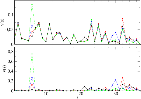
The transformation for the sector $s^{\prime}=34$ are shown in Fig. 25 for Cyprus (blue), Singapore (red), Luxembourg (green) and Malta (black). We see that for Luxembourg there is a strong transformation of $s^{\prime}=20$ to $s=6$ (publishing). At the same time the global profile, being different from the case of Fig. 24 with $s^{\prime}=2$, has similar features for different countries. The comparison with the transformation results from value exchange matrix $M_{ss^{\prime},cc^{\prime}}$ are again very different as in the case of Fig. 24.

The obtained results for the activity sector transformation by the WNEA open new possibilities for analysis of interactions between the world economic activities. The Google matrix approach provides new type of results being very different from usual Input/Output matrix approach. This is related to the fact that the transformation matrix (19) takes into account summation over various cycles over the network.

4 Discussion

In this work we have developed the Google matrix analysis of the world network of economic activities from the OECD-WTO TiVA database. The PageRank and CheiRank probabilities allowed to obtain ranking of world countries independently of their richness being mainly determined by the efficiency of their economic relations. The developed approach demonstrated the asymmetry in the economic activity sectors some of which are export oriented and others are import oriented. We also showed that the eigenstates of the WNEA Google matrix select specific quasi-isolated communities oriented to specific activity sectors. The CheiRank-PageRank balance $B_{c}$ allows to determine economically rising countries with robust network of economic relations. The sensitivity of this $B_{c}$ to price variations and labor cost in various countries determines the hidden relations between world economies being not visible via usual Export-Import exchange analysis. The Google matrix analysis determines also the transformation features of world activity sectors.

The comparison with the multiproduct world trade network from UN COMTRADE shows certain similarities between the two networks of WNEA and WTN. At the same time the WNEA data provides new elements for interactions of activity sectors while there are no direct interactions of products in COMTRADE database. From this viewpoint the OECD-WTO data captures the economic reality on a deeper level. But at the same time the OECD-WTO network is less developed compared to COMTRADE (less countries, years, sectors). Thus it is highly desirable to extend the OECD-WTO database.

We think that the Google matrix analysis developed here and in wtngoogle ; wtnproducts captures better the new reality of multifunctional directed tensor interactions and that the universal features of this approach can be also extended to multifunctional financial network flows which now attract an active interest of researchers craig ; garratt . Unfortunately, the data on financial flows have much less accessibility compared to the networks discussed here.

We point that recently some of the matrix methods, developed in physics community, started to find active application for economy systems (see e.g. bouchaud ; guhr ). However, usually for physicists these matrices have been from the unitary or Hermitian ensembles, where the Random Matrix Theory allowed to obtained certain universal results. Here, we show that the directed networks and tensors appearing in the interacting economy systems are described by the matrices of Perron-Frobenius operators which had not been studied much in physics. Thus the new field of research is now opened for physicists, mathematicians and computer scientists with application to complex interacting economy systems.

5 Acknowledgments

We thank the representatives of OECD oecd2014 and WTO wto2014 for providing us with the friendly access to the data sets investigated in this work. One of us (VK) thanks the Economic Research and Statistics Division, WTO Genève for hospitality during his intership there. We thank L.Ermann for useful discussions and advices on preparation of figures. This research is supported in part by the EC FET Open project “New tools and algorithms for directed network analysis” (NADINE $No$ 288956).

	country name	country code	country flag		country name	country code	country flag
1	Australia	AUS		30	Sweden	SWE
2	Austria	AUT		31	Switzerland	CHE
3	Belgium	BEL		32	Turkey	TUR
4	Canada	CAN		33	United Kingdom	GBR
5	Chile	CHL		34	United States	USA
6	Czech Republic	CZE		35	Argentina	ARG
7	Denmark	DNK		36	Brazil	BRA
8	Estonia	EST		37	China	CHN
9	Finland	FIN		38	Chinese Taipei	TWN
10	France	FRA		39	India	IND
11	Germany	DEU		40	Indonesia	IDN
12	Greece	GRC		41	Russia	RUS
13	Hungary	HUN		42	Singapore	SGP
14	Iceland	ISL		43	South Africa	ZAF
15	Ireland	IRL		44	Hong Kong	HKG
16	Israel	ISR		45	Malaysia	MYS
17	Italy	ITA		46	Phillippines	PHL
18	Japan	JPN		47	Thailand	THA
19	Korea	KOR		48	Romania	ROU
20	Luxembourg	LUX		49	Vietnam	VNM
21	Mexico	MEX		50	Saudi Arabia	SAU
22	Netherlands	NLD		51	Brunei Darussalam	BRN
23	New Zealand	NZL		52	Bulgaria	BGR
24	Norway	NOR		53	Cyprus	CYP
25	Poland	POL		54	Latvia	LVA
26	Portugal	PRT		55	Lithuania	LTU
27	Slovak Republic	SVK		56	Malta	MLT
28	Slovenia	SVN		57	Cambodia	KHM
29	Spain	ESP		58	Rest of the World	ROW

Table 1: List of $N_{c}=58$ countries (with rest of the world ROW) with country name, code and flag.

	OECD ICIO Category	ISIC Rev. 3 correspondence
1	C01T05 AGR	01 - Agriculture, hunting and related service activities 02 - Forestry, logging and related service activities 05 - Fishing, operation of fish hatcheries and fish farms; service activities incidental to fishing
2	C10T14 MIN	10 - Mining of coal and lignite; extraction of peat 11 - Extraction of crude petroleum and natural gas; service activities incidental to oil and gas extraction excluding surveying 12 - Mining of uranium and thorium ores 13 - Mining of metal ores 14 - Other mining and quarrying
3	C15T16 FOD	15 - Manufacture of food products and beverages 16 - Manufacture of tobacco products
4	C17T19 TEX	17 - Manufacture of textiles 18 - Manufacture of wearing apparel; dressing and dyeing of fur 19 - Tanning and dressing of leather; manufacture of luggage, handbags, saddlery, harness and footwear
5	C20 WOD	20 - Manufacture of wood and of products of wood and cork, except furniture; Manufacture of articles of straw and plaiting materials
6	C21T22 PAP	21 - Manufacture of paper and paper products 22 - Publishing, printing and reproduction of recorded media
7	C23 PET	23 - Manufacture of coke, refined petroleum products and nuclear fuel
8	C24 CHM	24 - Manufacture of chemicals and chemical products
9	C25 RBP	25 - Manufacture of rubber and plastics products
10	C26 NMM	26 - Manufacture of other non-metallic mineral products
11	C27 MET	27 - Manufacture of basic metals
12	C28 FBM	28 - Manufacture of fabricated metal products, except machinery and equipment
13	C29 MEQ	29 - Manufacture of machinery and equipment n.e.c.
14	C30 ITQ	30 - Manufacture of office, accounting and computing machinery
15	C31 ELQ	31 - Manufacture of electrical machinery and apparatus n.e.c.
16	C32 CMQ	32 - Manufacture of radio, television and communication equipment and apparatus
17	C33 SCQ	33 - Manufacture of medical, precision and optical instruments, watches and clocks
18	C34 MTR	34 - Manufacture of motor vehicles, trailers and semi-trailers
19	C35 TRQ	35 - Manufacture of other transport equipment
20	C36T37 OTM	36 - Manufacture of furniture; manufacturing n.e.c. 37 - Recycling
21	C40T41 EGW	40 - Electricity, gas, steam and hot water supply 41 - Collection, purification and distribution of water
22	C45 CON	45 - Construction
23	C50T52 WRT	50 - Sale, maintenance and repair of motor vehicles and motorcycles; retail sale of automotive fuel 51 - Wholesale trade and commission trade, except of motor vehicles and motorcycles 52 - Retail trade, except of motor vehicles and motorcycles; repair of personal and household goods
24	C55 HTR	55 - Hotels and restaurants
25	C60T63 TRN	60 - Land transport; transport via pipelines 61 - Water transport 62 - Air transport 63 - Supporting and auxiliary transport activities; activities of travel agencies
26	C64 PTL	64 - Post and telecommunications
27	C65T67 FIN	65 - Financial intermediation, except insurance and pension funding 66 - Insurance and pension funding, except compulsory social security 67 - Activities auxiliary to financial intermediation
28	C70 REA	70 - Real estate activities
29	C71 RMQ	71 - Renting of machinery and equipment without operator and of personal and household goods
30	C72 ITS	72 - Computer and related activities
31	C73 RDS	73 - Research and development
32	C74 BZS	74 - Other business activities
33	C75 GOV	75 - Public administration and defense; compulsory social security
34	C80 EDU	80 - Education
35	C85 HTH	85 - Health and social work
36	C90T93 OTS	90 - Sewage and refuse disposal, sanitation and similar activities 91 - Activities of membership organizations n.e.c. 92 - Recreational, cultural and sporting activities 93 - Other service activities
37	C95 PVH	95 - Private households with employed persons

Table 2: List of sectors considered by Input/Output matrices from OECD database, their correspondence to the ISIC classification is also given.

Sector	$\hat{K}$ (1995)	% vol (1995)	$\hat{K}^{*}$ (1995)	% vol (1995)	$\hat{K}$ (2008)	% vol (2008)	$\hat{K}^{*}$ (2008)	% vol (2008)
1	19	2.2979	16	2.9763	20	1.9532	16	2.0902
2	27	1.2993	2	8.6183	24	1.5245	1	15.8784
3	3	6.0117	12	3.3271	11	3.9327	17	1.9835
4	10	3.9579	14	3.0831	17	2.0934	19	1.8634
5	30	1.108	20	1.9037	33	0.60075	22	1.3001
6	11	3.5687	6	4.2128	18	2.0608	14	2.3736
7	4	5.9126	19	2.2783	1	11.589	4	6.34
8	2	6.251	1	10.6954	3	6.0558	2	9.1103
9	17	2.4035	15	3.0546	19	1.9785	13	2.5549
10	28	1.2	21	1.8337	29	1.0389	21	1.3177
11	8	4.4393	3	8.0658	4	5.4907	3	8.3184
12	20	2.2646	17	2.7194	23	1.6212	15	2.2182
13	9	4.0642	8	4.0365	9	4.0117	9	4.0597
14	12	3.3353	13	3.158	8	4.0642	6	5.0066
15	18	2.3789	9	4.0148	25	1.456	18	1.8673
16	15	2.7053	10	3.8054	14	2.7844	11	3.6339
17	31	1.0034	23	1.1434	34	0.31041	29	0.40161
18	7	5.2722	7	4.1643	6	5.1478	10	3.9907
19	26	1.3665	22	1.7813	26	1.3028	23	1.2752
20	24	1.6331	27	0.67546	22	1.6652	20	1.3858
21	21	2.1673	30	0.34377	10	3.946	30	0.39969
22	1	6.538	32	0.22022	2	6.8692	32	0.15209
23	5	5.8472	4	7.9296	7	4.6893	8	4.6745
24	25	1.5283	29	0.37682	27	1.2377	27	0.62202
25	6	5.8385	5	6.5023	5	5.2454	5	5.8065
26	29	1.1862	26	0.6839	28	1.2179	26	0.62929
27	13	2.7584	18	2.3006	15	2.5623	12	3.3487
28	33	0.70446	24	0.93849	31	0.84772	33	0.105
29	36	0.16329	33	0.18955	36	0.21276	24	0.81082
30	34	0.53799	28	0.39581	32	0.67481	28	0.61668
31	35	0.36919	31	0.33351	35	0.24684	31	0.24177
32	16	2.618	11	3.372	13	3.0455	7	4.7163
33	14	2.7071	34	0.064931	12	3.3939	35	0.06377
34	32	0.89993	36	0.0416	30	1.036	34	0.09439
35	22	1.8912	35	0.045551	16	2.2601	36	0.025979
36	23	1.7326	25	0.7136	21	1.8131	25	0.72283
37	37	0.03899	37	0	37	0.019524	37	0

Table 3: First column gives the sectors from OECD database, for each of them the following columns give the ImportRank $\hat{K}$ with the sector fraction in global trade value and ExportRank $\hat{K}^{*}$ with sector fraction in global trade value. Data are shown for 1995 and 2008.

	$K$	$K^{*}$	$K_{2}$	$\hat{K}$	$\hat{K}^{*}$
1	DEU C34 MTR	ROW C10T14 MIN	DEU C24 CHM	USA C23 PET	ROW C10T14 MIN
2	USA C75 GOV	RUS C10T14 MIN	USA C65T67 FIN	JPN C23 PET	SAU C10T14 MIN
3	ROW C75 GOV	SAU C10T14 MIN	DEU C29 MEQ	USA C75 GOV	RUS C10T14 MIN
4	SAU C85 HTH	USA C24 CHM	DEU C34 MTR	ROW C45 CON	USA C24 CHM
5	GBR C85 HTH	DEU C24 CHM	DEU C27 MET	CHN C32 CMQ	CAN C10T14 MIN
6	USA C34 MTR	DEU C27 MET	USA C74 BZS	CHN C27 MET	DEU C24 CHM
7	ROW C45 CON	NOR C10T14 MIN	DEU C50T52 WRT	USA C45 CON	NOR C10T14 MIN
8	ROW C15T16 FOD	RUS C27 MET	USA C24 CHM	DEU C34 MTR	AUS C10T14 MIN
9	USA C15T16 FOD	USA C50T52 WRT	DNK C60T63 TRN	KOR C23 PET	CHN C30 ITQ
10	RUS C50T52 WRT	DEU C29 MEQ	GBR C74 BZS	DEU C23 PET	USA C30 ITQ
11	USA C45 CON	USA C74 BZS	JPN C34 MTR	JPN C40T41 EGW	JPN C30 ITQ
12	USA C85 HTH	CHN C27 MET	GBR C65T67 FIN	ROW C75 GOV	DEU C29 MEQ
13	DEU C15T16 FOD	USA C60T63 TRN	CHN C32 CMQ	CHN C24 CHM	DEU C34 MTR
14	ROW C60T63 TRN	GBR C65T67 FIN	CHN C24 CHM	USA C34 MTR	KOR C32 CMQ
15	USA C65T67 FIN	USA C23 PET	DEU C60T63 TRN	USA C24 CHM	USA C23 PET
16	GBR C50T52 WRT	GBR C74 BZS	FRA C50T52 WRT	CHN C30 ITQ	USA C74 BZS
17	DEU C24 CHM	USA C65T67 FIN	USA C50T52 WRT	CHN C23 PET	TWN C32 CMQ
18	DEU C29 MEQ	CHN C30 ITQ	CHN C50T52 WRT	ROW C60T63 TRN	CHN C27 MET
19	DEU C50T52 WRT	DEU C34 MTR	CHN C29 MEQ	CHN C29 MEQ	DEU C27 MET
20	DEU C27 MET	USA C30 ITQ	ROW C60T63 TRN	DEU C29 MEQ	GBR C74 BZS

Table 4: Top 20 ranks for global PageRank $K$, CheiRank$K^{*}$, 2DRank $K_{2}$, ImportRank $K$ and ExportRank $K^{*}$ for the year 2008.

$K_{i}$	$|\psi_{i}|$	node	$|\psi_{i}|$	node	$|\psi_{i}|$	node	$|\psi_{i}|$	node
1	0.037606	ROW C17T19 TEX	0.050431	ARG C34 MTR	0.054681	CHN C32 CMQ	0.052248	RUS C10T14 MIN
2	0.025695	CHN C17T19 TEX	0.049991	BRA C34 MTR	0.053306	KOR C32 CMQ	0.03948	SAU C10T14 MIN
3	0.021618	ITA C17T19 TEX	0.029753	JPN C34 MTR	0.053253	TWN C32 CMQ	0.026187	ROW C10T14 MIN
4	0.017075	USA C17T19 TEX	0.026592	DEU C34 MTR	0.027361	SGP C32 CMQ	0.022125	NOR C10T14 MIN
5	0.016216	CHN C32 CMQ	0.018372	THA C34 MTR	0.025189	MYS C32 CMQ	0.019764	USA C71 RMQ
6	0.013003	CHN C30 ITQ	0.01531	IDN C34 MTR	0.018824	USA C30 ITQ	0.013899	USA C50T52 WRT
7	0.010963	FRA C17T19 TEX	0.0093875	ROW C21T22 PAP	0.016965	PHL C32 CMQ	0.011638	ROW C29 MEQ
8	0.010175	TUR C17T19 TEX	0.0093382	DEU C15T16 FOD	0.01534	JPN C30 ITQ	0.010871	RUS C27 MET
9	0.010161	USA C75 GOV	0.0090288	USA C15T16 FOD	0.014664	GBR C65T67 FIN	0.0082943	DEU C29 MEQ
10	0.0099839	USA C65T67 FIN	0.0086552	USA C75 GOV	0.013713	CHN C30 ITQ	0.0082905	RUS C23 PET

Table 5: Top 10 values of 4 different eigenvectors from Fig.9, Fig. 10. The corresponding eigenvalues from left to right are $\lambda=0.4993$ (red), $\lambda=0.3746+0.0126i$ (green), $\lambda=0.6256$ (blue) and $\lambda=-0.0001+0.1687i$ (magenta).