A posteriori error analysis of round-off errors in the numerical solution of ordinary differential equations

Abstract

We prove sharp, computable error estimates for the propagation of errors in the numerical solution of ordinary differential equations. The new estimates extend previous estimates of the influence of data errors and discretisation errors with a new term accounting for the propagation of numerical round-off errors, showing that the accumulated round-off error is inversely proportional to the square root of the step size. As a consequence, the numeric precision eventually sets the limit for the pointwise computability of accurate solutions of any ODE. The theoretical results are supported by numerically computed solutions and error estimates for the Lorenz system and the van der Pol oscillator.

1 Introduction

We consider the numerical solution of general initial value problems for systems of ordinary differential equations (ODE),

$$\begin{split}\dot{u}(t)&=f(u(t),t),\quad t\in(0,T],\\ u(0)&=u_{0},\end{split}$$ (1)

where the right-hand side $f:\mathbb{R}^{N}\times[0,T]\rightarrow\mathbb{R}^{N}$ is assumed to be Lipschitz continuous in $u$ and continuous in $t$. Our objective is to analyse the error in an approximate solution $U:[0,T]\rightarrow\mathbb{R}^{N}$ computed by a single-step numerical method, such as an explicit or implicit Runge–Kutta method. For the numerical results presented at the end of this work, we have used a time-stepping method formulated as a Galerkin finite element method — which, for any particular choice of finite element basis and quadrature, will correspond to a particular implicit Runge–Kutta method — but stress that the theoretical results are not particular to time-stepping based on Galerkin formulations but generic to all single-step methods.

The propagation of local errors and accumulation of global errors in the numerical solution of ODE have been studied extensively in the literature, see e.g. eriksson_introduction_1995 ; estep_global_1994 ; estep_posteriori_1995 ; estep_pointwise_1998 ; cao2004posteriori . These estimates are based on the formulation of an auxiliary dual problem: the linearised adjoint problem. From the solution of the dual problem, the accumulation rate of local errors may be computed, either as global stability factors or as local stability weights. These factors or weights, together with a measure of the local error, typically the residual $R(t)=\dot{U}-f(U(t),t)$ lead to a computable estimate of the global error.

Standard estimates may include various sources contributing to the global error, such as discretisation errors, accounting for the use of finite time steps, quadrature errors, accounting for the approximation of the right-hand side $f$ by a particular quadrature rule, and data errors, accounting for the approximation of the initial value $u_{0}$. In this work, we extend these estimates by adding a new term accounting for the use of finite numeric precision in the computation of the numerical solution. This error is normally neglected, since it is typically much smaller than the contribution from the data or discretisation error. However, when the system (1) is very sensitive to perturbations, when the time interval $[0,T]$ is very long, or when a solution is sought with very high accuracy, the effect of numerical round-off errors as a result of finite numeric precision can and will be the dominating error source, which ultimately limits the computability of a given problem.

2 Main result

We prove below that the error $\mathbf{E}$ in a computed numerical solution $U$ approximating the exact solution $u$ of the ODE (1) is the sum of three contributions:

$$\mathbf{E}=\mathbf{E}_{D}+\mathbf{E}_{G}+\mathbf{E}_{C},$$

where $\mathbf{E}_{D}$ is the data error, which is nonzero if $U(0)\neq u(0)$; $\mathbf{E}_{G}$ is the discretisation error, which is nonzero as a result of a finite time step; and $\mathbf{E}_{C}$ is the computational error, which is nonzero as a result of finite numerical precision. Furthermore, we bound each of the three contributions as the product of a stability factor and a residual that measures the size of local contributions to the error. The size of the residuals may be estimated in terms of the size of the time step. We find that

$$\mathbf{E}\sim S_{D}(T)\|U(0)-u(0)\|+S_{G}(T)\Delta{}t^{r}+S_{C}(T)\Delta{}t^{-1/2},$$

where $\Delta{}t$ is the size of the time step, $r$ the order of convergence of the numerical method, and $S_{D}(T)$, $S_{G}(T)$, $S_{C}(T)$ are stability factors which can be computed a posteriori.

3 Error analysis

The error analysis is based on the solution of an auxiliary dual problem and follows the now well established techniques developed in estep_global_1994 , estep_posteriori_1995 , eriksson_introduction_1995 and becker_optimal_2001 , with extensions to account for the accumulation of round-off errors.

The dual (linearised adjoint) problem takes the form of an initial value problem for a system of linear ordinary differential equations:

$$\begin{split}-\dot{z}(t)&=\bar{A}^{\top}(t)z(t),\quad t\in[0,T),\\ z(T)&=z_{T}.\end{split}$$ (2)

Here, $\bar{A}$ denotes the Jacobian matrix of the right-hand side $f$ averaged over the approximate solution $U$ and the exact solution $u$:

$$\bar{A}(t)=\int_{0}^{1}\frac{\partial f}{\partial u}(sU(t)+(1-s)u(t),t)\,\mathrm{d}s.$$ (3)

By the chain rule, it follows that

$$\begin{split}\bar{A}(t)(U(t)-u(t))&=\int_{0}^{1}\frac{\partial f}{\partial u}(sU(t)+(1-s)u(t),t)(U(t)-u(t))\,\mathrm{d}s\\ &=\int_{0}^{1}\frac{\partial}{\partial s}f(sU(t)+(1-s)u(t),t)\,\mathrm{d}s=f(U(t),t)-f(u(t),t).\end{split}$$

Based on the formulation of the dual problem we may now derive a (standard) error representation (Theorem 3.1). It represents the error in an approximate solution $U$ (computed by any numerical method) in terms of the residual $R$ of the computed solution and the solution $z$ of the dual problem (2). The only assumption we make on the numerical solution $U$ is that it is piecewise smooth on a partition of the interval $[0,T]$ (or that it may be extended to such a function). At points where $U$ is smooth, the residual is defined by

$$R(t)=\dot{U}(t)-f(U(t),t).$$

Theorem 3.1 (Error representation)

Let $u:[0,T]\rightarrow\mathbb{R}^{N}$ be the exact solution of the initial value problem (1), let $z:[0,T]\rightarrow\mathbb{R}^{N}$ be the solution of the dual problem (2), and let $U:[0,T]\rightarrow\mathbb{R}^{N}$ be any piecewise smooth approximation of $u$ on a partition $0=t_{0}<t_{1}<\cdots<t_{M}=T$ of $[0,T]$, that is, $U|_{(t_{m-1},t_{m}]}\in\mathcal{C}^{\infty}((t_{m-1},t_{m}])$ for $m=1,2,\ldots,M$ ($U$ is left-continuous). Then, the error $U(T)-u(T)$ may be represented by

$$\langle z_{T},U(T)-u(T)\rangle=\langle z(0),U(0)-u(0)\rangle+\sum_{m=1}^{M}\langle z(t_{m-1}),[U]_{m-1}\rangle+\int_{0}^{T}\langle z,R\rangle\,\mathrm{d}t,$$

where $R(t)=\dot{U}(t)-f(U(t),t)$ is the residual of the approximate solution $U$ and $[U]_{m-1}=U(t_{m-1}^{+})-U(t_{m-1})=\lim_{t\rightarrow t_{m-1}^{+}}U(t)-U(t_{m-1})$.

Proof

By the definition of the dual problem, we find that

$$\langle z_{T},e(T)\rangle=\langle z_{T},e(T)\rangle-\int_{0}^{T}\langle\dot{z}+\bar{A}^{\top}z,e\rangle\,\mathrm{d}t=\langle z_{T},e(T)\rangle-\sum_{m=1}^{M}\int_{t_{m-1}}^{t_{m}}\langle\dot{z}+\bar{A}^{\top}z,e\rangle\,\mathrm{d}t,$$

where $e=U-u$. Noting that $\langle\bar{A}^{\top}z,e\rangle=\langle z,\bar{A}e\rangle$ and integrating by parts, we obtain

$$\langle z_{T},e(T)\rangle=\langle z(0),e(0)\rangle+\sum_{m=1}^{M}\left[\langle z(t_{m-1}),[U]_{m-1}\rangle+\int_{t_{m-1}}^{t_{m}}\langle z,\dot{e}-\bar{A}e\rangle\,\mathrm{d}t\right],$$

where $[U]_{m-1}=U(t_{m-1}^{+})-U(t_{m-1}^{-})=U(t_{m-1}^{+})-U(t_{m-1})$ denotes the jump of $U$ at $t=t_{m-1}$. By the construction of $\bar{A}$, it follows that $\bar{A}e=f(U,\cdot)-f(u,\cdot)$. Hence, $\dot{e}-\bar{A}e=\dot{U}-f(U,\cdot)-\dot{u}+f(u,\cdot)=\dot{U}-f(U,\cdot)=R$, which completes the proof.

Remark 1

Theorem 3.1 holds for any piecewise smooth function $U:[0,T]\rightarrow\mathbb{R}^{N}$, in particular for any piecewise smooth extension of any approximate numerical solution obtained by any numerical method for (1).

We next investigate the contribution to the error in the computed numerical solution $U$ from errors in initial data, numerical discretisation, and computation (round-off errors), $\mathbf{E}=\mathbf{E}_{D}+\mathbf{E}_{G}+\mathbf{E}_{C}$, and derive sharp bounds for each term.

To estimate the computational error, we introduce the discrete residual $\bar{R}$ defined as follows. For any $p\geq 0$, let $\{\lambda_{k}\}_{k=0}^{p}$ be the Lagrange nodal basis for $\mathcal{P}^{p}([0,1])$, the space of polynomials of degree $\leq p$ on $[0,1]$, on a partition $0\leq\tau_{0}<\tau_{1}<\cdots<\tau_{p}\leq 1$ of $[0,1]$, that is, $\mathrm{span}\{\lambda_{k}\}_{k=0}^{p}=\mathcal{P}^{p}([0,1])$ and $\lambda_{i}(\tau_{j})=\delta_{ij}$. Then, the discrete residual $\bar{R}_{k}$ is defined on each interval $(t_{m-1},t_{m}]$ by

$$\bar{R}_{k}^{m}=\lambda_{k}(0)[U]_{m-1}+\int_{t_{m-1}}^{t_{m}}\lambda_{k}((t-t_{m-1})/\Delta{}t_{m})R(t)\,\mathrm{d}t,\quad k=0,1,\ldots,p.$$ (4)

We also define the corresponding interpolation operator $\pi$ onto the space of piecewise polynomial functions on the partition $0=t_{0}<t_{1}<\cdots<t_{M}=T$ by

$$(\pi v)(t)=\sum_{k=0}^{p}v(t_{m-1}+\tau_{k}\Delta{}t_{m})\,\lambda_{k}((t-t_{m-1})/\Delta{}t_{m}),\quad t\in(t_{m-1},t_{m}].$$

We may now prove the following a posteriori error estimate.

Theorem 3.2 (Error estimate)

Let $u:[0,T]\rightarrow\mathbb{R}^{N}$ be the exact solution of the initial value problem (1), let $z:[0,T]\rightarrow\mathbb{R}^{N}$ be the solution of the dual problem (2), and let $U:[0,T]\rightarrow\mathbb{R}^{N}$ be any piecewise smooth approximation of $u$ on a partition $0=t_{0}<t_{1}<\cdots<t_{M}=T$ of $[0,T]$, that is, $U|_{(t_{m-1},t_{m}]}\in\mathcal{C}^{\infty}((t_{m-1},t_{m}])$ for $m=1,2,\ldots,M$ ($U$ is left-continuous). Then, for any $p\geq 0$, the following error estimate holds:

$$\langle z_{T},U(T)-u(T)\rangle=\mathbf{E}_{D}+\mathbf{E}_{G}+\mathbf{E}_{C},$$ (5)

where

$$\begin{split}|\mathbf{E}_{D}|&\leq S_{D}\,\|U(0)-u(0)\|,\\ |\mathbf{E}_{G}|&\leq S_{G}\,C_{p}\max_{[0,T]}\left\{\Delta{}t^{p+1}(\|[U]\|/\Delta{}t+\|R\|)\right\},\\ |\mathbf{E}_{C}|&\leq S_{C}\,C_{p}^{\prime}\max_{0\leq k\leq p}\max_{[0,T]}\|\Delta{}t^{-1}\bar{R}_{k}\|.\end{split}$$

Here, $C_{p}$ and $C_{p}^{\prime}$ are constants depending only on $p$. The stability factors $S_{D}$, $S_{G}$, and $S_{C}$ are defined by

$$\begin{split}S_{D}&=\|z(0)\|,\\ S_{G}&=\int_{0}^{T}\|z^{(p+1)}\|\,\mathrm{d}t,\\ S_{C}&=\int_{0}^{T}\|\pi z\|\,\mathrm{d}t.\end{split}$$

Proof

Starting from the error representation of Theorem 3.1, we add and subtract the degree $p$ left-continuous piecewise polynomial interpolant $\pi z$ defined above to obtain

$$\begin{split}\langle z_{T},e(T)\rangle&=\langle z(0),e(0)\rangle\\ &\quad+\sum_{m=1}^{M}\left[\langle z(t_{m-1})-\pi z(t_{m-1}^{+}),[U]_{m-1}\rangle+\int_{t_{m-1}}^{t_{m}}\langle z-\pi z,R\rangle\,\mathrm{d}t\right]\\ &\quad+\sum_{m=1}^{M}\left[\langle\pi z(t_{m-1}^{+}),[U]_{m-1}\rangle+\int_{t_{m-1}}^{t_{m}}\langle\pi z,R\rangle\,\mathrm{d}t\right]\\ &\equiv\mathbf{E}_{D}+\mathbf{E}_{G}+\mathbf{E}_{C}.\end{split}$$

We first note that the data error $\mathbf{E}_{D}$ is bounded by $\|z(0)\|\,\|e(0)\|\equiv S_{D}\,\|e(0)\|$. By an interpolation estimate, we may estimate the discretisation error $\mathbf{E}_{G}$ by

$$\begin{split}\mathbf{E}_{G}&\leq\sum_{m=1}^{M}\left[\|z(t_{m-1})-\pi z(t_{m-1}^{+})\|\,\|[U]_{m-1}\|+\int_{t_{m-1}}^{t_{m}}\|z-\pi z\|\,\|R\|\,\mathrm{d}t\right]\\ &\leq C_{p}\max_{[0,T]}\left\{\Delta{}t^{p+1}(\|[U]\|/\Delta{}t+\|R\|)\right\}\sum_{m=1}^{M}\int_{t_{m-1}}^{t_{m}}\|z^{(p+1)}\|\,\mathrm{d}t,\end{split}$$

where $\sum_{m=1}^{M}\int_{t_{m-1}}^{t_{m}}\|z^{(p+1)}\|\,\mathrm{d}t=\int_{0}^{T}\|z^{(p+1)}\|\,\mathrm{d}t\equiv S_{G}$ and $C_{p}$ is an interpolation constant. Finally, to estimate the computational error, we expand $\pi z$ in the nodal basis to obtain

$$\begin{split}\mathbf{E}_{C}&=\sum_{m=1}^{M}\sum_{k=0}^{p}\left\langle z(t_{m-1}+\tau_{k}\Delta{}t_{m}),\lambda_{k}(0){[U]_{m-1}}+\int_{t_{m-1}}^{t_{m}}\lambda_{k}((t-t_{m-1})/\Delta{}t_{m})R(t)\,\mathrm{d}t\right\rangle\\ &=\sum_{m=1}^{M}\sum_{k=0}^{p}\langle z(t_{m-1}+\tau_{k}\Delta{}t_{m}),\bar{R}_{k}^{m}\rangle=\sum_{m=1}^{M}\Delta{}t_{m}\sum_{k=0}^{p}\langle z(t_{m-1}+\tau_{k}\Delta{}t_{m}),\Delta{}t_{m}^{-1}\bar{R}_{k}^{m}\rangle\\ &\leq\sum_{m=1}^{M}\Delta{}t_{m}\sum_{k=0}^{p}\|z(t_{m-1}+\tau_{k}\Delta{}t_{m})\|\,\|\Delta{}t_{m}^{-1}\bar{R}_{k}^{m}\|\\ &\leq\max_{0\leq k\leq p}\max_{[0,T]}\|\Delta{}t^{-1}\bar{R}_{k}\|\sum_{m=1}^{M}\Delta{}t_{m}\sum_{k=0}^{p}\|z(t_{m-1}+\tau_{k}\Delta{}t_{m})\|\\ &\leq C_{p}^{\prime}\max_{0\leq k\leq p}\max_{[0,T]}\|\Delta{}t^{-1}\bar{R}_{k}\|\sum_{m=1}^{M}\int_{t_{m-1}}^{t_{m}}\|\pi z\|\,\mathrm{d}t,\end{split}$$

where $\sum_{m=1}^{M}\int_{t_{m-1}}^{t_{m}}\|\pi z\|\,\mathrm{d}t=\int_{0}^{T}\|\pi z\|\,\mathrm{d}t\equiv S_{C}$ and $C_{p}^{\prime}$ is a constant depending only on $p$. This completes the proof.

Remark 2

Theorem 3.2 estimates the size of $\langle z_{T},U(T)-u(T)\rangle$ for any given vector $z_{T}$. We may thus estimate any bounded linear functional of the error at the final time by choosing $z_{T}$ as the corresponding Riesz representer. In particular, we may estimate the error in any component $u_{i}(T)$ of the solution by setting $z_{T}$ to the $i$th unit vector for $i=1,2,\ldots,N$.

Theorem 3.2 extends standard a posteriori error estimates for systems of ordinary differential equations in two ways. First, it does not make any assumption on the underlying numerical method. Second, it includes the effect of numerical round-off errors. A similar estimate can be found in logg_multi-adaptive_2003-1 but only for the simplest case of the piecewise linear $\mathrm{cG}(1)$ method (Crank–Nicolson).

We now investigate the propagation of numerical round-off errors in more detail. As in the proof of Theorem 3.2, $\mathbf{E}_{C}$ denotes the computational error defined by

$$\mathbf{E}_{C}=\sum_{m=1}^{M}\left[\langle\pi z(t_{m-1}^{+}),[U]_{m-1}\rangle+\int_{t_{m-1}}^{t_{m}}\langle\pi z,R\rangle\,\mathrm{d}t\right].$$ (6)

Theorem 3.2 bounds the computational error in terms of the discrete residual defined in (4). The discrete residual tests the continuous residual $R=\dot{U}-f$ of (1) against polynomials of degree $p$. In particular, it tests how well the numerical method satisfies the relation

$$U(t_{m})=U(t_{m-1})+\int_{t_{m-1}}^{t_{m}}f(U,\cdot)\,\mathrm{d}t.$$ (7)

With a machine precision of size $\epsilon_{\textrm{mach}}$, our best hope is that the numerical method satisfies (7) to within a tolerance of size $\epsilon_{\textrm{mach}}$ for each component of the vector $U$. It follows by the Cauchy–Schwarz inequality that

$$\max_{k,m}\|\bar{R}_{k}^{m}\|\leq\epsilon_{\textrm{mach}}\sqrt{N}.$$

We thus have the following corollary.

Corollary 1

The computational error $\mathbf{E}_{C}$ of Theorem 3.2 is bounded by

$$|\mathbf{E}_{C}|\leq S_{C}\,C_{p}^{\prime}\frac{\epsilon_{\textrm{mach}}\sqrt{N}}{\min_{[0,T]}\Delta{}t}.$$

This indicates that the computational error scales like $\Delta{}t^{-1}$; the smaller the time step, the larger the computational error. At first, this seems non-intuitive, but it is a simple consequence of the fact that a smaller time step leads to a larger number of time steps and thus a larger number of round-off errors.

The estimate of Corollary 1 is overly pessimistic. It is based on the assumption that round-off errors accumulate without cancellation. In practice, the round-off error is sometimes positive and sometimes negative. As a simple model, we make the assumption that the round-off error is a random variable which takes the value $+\epsilon_{\textrm{mach}}$ or $-\epsilon_{\textrm{mach}}$ with equal probabilities,

$$(\bar{R}_{k}^{m})_{i}=\left\{\begin{array}[]{rcl}+\epsilon_{\textrm{mach}},&&p=0.5,\\ -\epsilon_{\textrm{mach}},&&p=0.5,\\ \end{array}\right.$$ (8)

for all $m,k,i$. In reality, round-off errors are not uncorrelated random variables, but the simple model (8) may still give useful results. For a discussion on the applicability of random models to the propagation of round-off errors, see higham2002accuracy (Section 2.8) and Hairer2008 .

Under the assumption (8), we find that the expected size of the computational error scales like $\Delta{}t^{-1/2}$. As we shall see in the next section, this is also confirmed by numerical experiments. A similar result is obtained in a series of papers by Li et. al li2000 ; li2001 . In li2000 , it is first noted that there exists an optimal time step; that is, a time step for which discretisation errors and round-off errors balance. In li2001 , it is then found that the round-off error is inversely proportional to the square root of the time step. These results are confirmed by the following theorem.

Theorem 3.3

Assume that the round-off error is a random variable of size $\pm\epsilon_{\textrm{mach}}$ with equal probabilities. Then the root-mean squared expected computational error $\mathbf{E}_{C}$ of Theorem 3.2 is bounded by

$$(E[\mathbf{E}_{C}^{2}])^{1/2}\leq S_{{C_{2}}}\,\sqrt{C_{p}^{\prime}}\frac{\epsilon_{\textrm{mach}}}{\min_{[0,T]}\sqrt{\Delta{}t}},$$

where $S_{C_{2}}=\left(\int_{0}^{T}\|\pi z\|^{2}\,\mathrm{d}t\right)^{1/2}$ and $C_{p}^{\prime}$ is a constant depending only on $p$.

Proof

As in the proof of Theorem 3.2, we obtain

$$\mathbf{E}_{C}=\sum_{m=1}^{M}\sum_{k=0}^{p}\langle z(t_{m-1}+\tau_{k}\Delta{}t_{m}),\bar{R}_{k}^{m}\rangle=\sum_{m=1}^{M}\sum_{k=0}^{p}\sum_{i=1}^{N}z_{i}(t_{m-1}+\tau_{k}\Delta{}t_{m})(\bar{R}_{k}^{m})_{i},$$

where by assumption $(\bar{R}_{k}^{m})_{i}=\epsilon_{\textrm{mach}}x_{mki}$ and $x_{mki}=\pm 1$ with probability $0.5$ and $0.5$, respectively. It follows that

$$\begin{split}\mathbf{E}_{C}^{2}&=\sum_{m,n=1}^{M}\sum_{k,l=0}^{p}\sum_{i,j=1}^{N}z_{i}(t_{m-1}+\tau_{k}\Delta{}t_{m})z_{j}(t_{n-1}+\tau_{l}\Delta{}t_{n})\,\epsilon_{\textrm{mach}}^{2}x_{mki}x_{nlj}\\ &=\sum_{(m,k,i)=(n,l,j)}z_{i}^{2}(t_{m-1}+\tau_{k}\Delta{}t_{m})\,\epsilon_{\textrm{mach}}^{2}x_{mki}^{2}\\ &+\sum_{(m,k,i)\neq(n,l,j)}z_{i}(t_{m-1}+\tau_{k}\Delta{}t_{m})z_{j}(t_{n-1}+\tau_{l}\Delta{}t_{n})\,\epsilon_{\textrm{mach}}^{2}x_{mki}x_{nlj}.\end{split}$$

We now note that $x_{mki}^{2}=1$. Furthermore, $y_{ijklmn}=x_{mki}x_{nlj}$ is a random variable which takes the values $+1$ and $-1$ with equal probabilities. We thus find that

$$\begin{split}E[\mathbf{E}_{C}^{2}]&=\epsilon_{\textrm{mach}}^{2}\sum_{m=1}^{M}\sum_{k=0}^{p}\sum_{i=1}^{N}z_{i}^{2}(t_{m-1}+\tau_{k}\Delta{}t_{m})+0\\ &=\epsilon_{\textrm{mach}}^{2}\sum_{m=1}^{M}\sum_{k=0}^{p}\|z(t_{m-1}+\tau_{k}\Delta{}t_{m})\|^{2}\\ &\leq\frac{\epsilon_{\textrm{mach}}^{2}}{\min_{[0,T]}\Delta{}t}\sum_{m=1}^{M}\Delta{}t_{m}\sum_{k=0}^{p}\|z(t_{m-1}+\tau_{k}\Delta{}t_{m})\|^{2}\leq S_{{C_{2}}}^{2}\,C_{p}^{\prime}\frac{\epsilon_{\textrm{mach}}^{2}}{\min_{[0,T]}\Delta{}t},\end{split}$$

where $S_{C_{2}}=\left(\int_{0}^{T}\|\pi z\|^{2}\,\mathrm{d}t\right)^{1/2}$. This completes the proof.

Remark 3

By additional assumptions on the smoothness of the dual solution $z$, one may relate the error to the expected value of the distance from the starting point for a random walk which is $\sqrt{n}$ for $n$ steps (for $n$ large), and prove a similar estimate for the expected absolute value of the computational error, $E[|\mathbf{E}_{C}|]\sim S_{C}\epsilon_{\textrm{mach}}/\sqrt{\Delta{}t}$, where $S_{C}=\int_{0}^{T}\|\pi z\|\,\mathrm{d}t$.

Remark 4

By Cauchy–Schwarz, the stability factor $S_{C}$ of Theorem 3.2 is bounded by $\sqrt{T}S_{C_{2}}$.

Remark 5

In Hairer2008 , the effect of numerical round-off error accumulation and its relation to Brownian motion (Brouwer’s law) are discussed in the context of symplectic methods for Hamiltonian systems. It should be noted that although the assumptions of Theorem 3.3 are similar to those in Hairer2008 , namely that the process of error accumulation for round-off errors is random rather than systematic, the point under discussion in the present work is different: the effect of time step size rather than the effect of the interval length.

We conclude this section by discussing how the above error estimates apply to the particular methods used in this work. The estimate of Theorem 3.2 is valid for any numerical method but is of particular interest as an a posteriori error estimate for the finite element methods $\mathrm{cG}(q)$ and $\mathrm{dG}(q)$ (see hulme_discrete_1972 ; hulme_one-step_1972 ; johnson_error_1988 ; delfour_discontinuous_1981 ).

The continuous and discontinuous Galerkin methods $\mathrm{cG}(q)$ and $\mathrm{dG}(q)$ are formulated by requiring that the residual $R=\dot{U}-f(U,\cdot)$ be orthogonal to a suitable space of test functions. By making a piecewise polynomial ansatz, the solution may be computed on a sequence of intervals partitioning the computational domain $[0,T]$ by solving a system of equations for the degrees of freedom on each consecutive interval. For a particular choice of numerical quadrature and degree $q$, the $\mathrm{cG}(q)$ and $\mathrm{dG}(q)$ methods both reduce to standard implicit Runge–Kutta methods.

In the case of the $\mathrm{cG}(q)$ method, the numerical solution $U$ is a continuous piecewise polynomial of degree $q$ that on each interval $(t_{n-1},t_{n}]$ satisfies

$$\int_{t_{n-1}}^{t_{n}}v\,R\,\mathrm{d}t=0$$ (9)

for all $v\in\mathcal{P}^{q-1}([t_{n-1},t_{n}])$. It follows that the discrete residual (4) is zero if $p\leq q-1$. However, this is only true in exact arithmetic. In practice, the discrete residual is nonzero and measures how well we solve the $\mathrm{cG}(q)$ equations (9), including round-off errors and errors from numerical quadrature. For the $\mathrm{cG}(q)$ method, we further expect the residual to converge as $\Delta{}t^{q}$. Thus, choosing $p=q-1$ in Theorem 3.2, one may expect the error for the $\mathrm{cG}(q)$ method to scale as

$$E=\mathbf{E}_{D}+\mathbf{E}_{G}+\mathbf{E}_{C}\sim S(T)\left(\epsilon_{\textrm{mach}}+\Delta{}t^{2q}+\Delta{}t^{-1/2}\epsilon_{\textrm{mach}}\right).$$ (10)

Here, $S(T)$ denotes a generic stability factor. As in Theorem 3.2, each term contributing to the total error is in reality multiplied by a particular stability factor. In practice, however, the growth rates of the different stability factors are similar and related by a constant factor.

4 Numerical results

In this section, we present numerical results in support of Theorem 3.2 and Theorem 3.3. The examples are the well-known Lorenz system and Van der Pol oscillator. Both examples illustrate the competing convergence rates for discretisation errors, decreasing rapidly for smaller time steps, and computational errors (round-off error), increasing for smaller time steps.

The numerical results were obtained using the authors’ software package Tanganyika tanganyika-web which implements the methods described in logg_multi-adaptive_2003-1 using high precision numerics provided by GMP Granlund15 . A complete code for reproducing all results in this paper is available at kehlet_2015_16671 . For details on the implementation, see kehlet_analysis_2010 .

4.1 The Lorenz system

We first consider the well-known Lorenz system lorenz_deterministic_1963 , a simple system of three ordinary differential equations exhibiting rapid amplification of numerical errors:

$$\left\{\begin{aligned} \dot{x}&=\sigma(y-x),\\ \dot{y}&=rx-y-xz,\\ \dot{z}&=xy-bz,\\ \end{aligned}\right.$$ (11)

where $\sigma=10$, $b=8/3$, and $r=28$. We take $u(0)=(1,0,0)$.

The Lorenz system is deterministically chaotic. In the context of a posteriori error analysis of numerical methods for the solution of ODE initial value problems, as in the present work, this means that solutions may, in principle, be computed over arbitrarily long time intervals, but to a rapidly increasing cost as function of the final time $T$.

4.1.1 Computability and growth of stability factors

In estep_pointwise_1998 , computability was demonstrated and quantified for the Lorenz on time intervals of moderate length ($T=30$) on a standard desktop computer. This result was further extended to time $T=48$ in logg_multi-adaptive_2003 , using high order ($\|e(T)\|\sim\Delta{}t^{30}$) finite element methods. Solutions over longer time intervals have been computed based on shadowing (the existence of a nearby exact solution), see coomes_rigorous_1995 , but for unknown initial data. Related work on high-precision numerical methods applied to the Lorenz system include viswanath2004fractal and jorba_software_2005 .

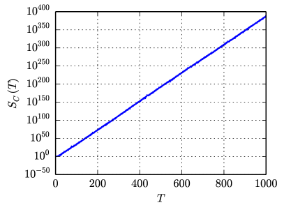
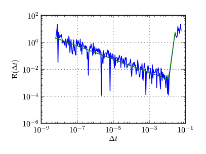
In KehletLogg2014 , the authors study the computability of the Lorenz system in detail on the time interval $[0,1000]$. Computability is here defined as the maximal final time $T=T(\epsilon_{\textrm{mach}})$ such that a solution may be computed with a given machine precision $\epsilon_{\textrm{mach}}$. The computability may be estimated by examining the growth rate of the stability factors appearing in the error estimate of Theorem 3.2. By numerical solution of the dual problem, it was found in KehletLogg2014 that the stability factors grow exponentially as $S(T)\sim 10^{0.388T}\sim 10^{0.4T}$; see Figure 1.

Figure 1: Growth of the stability factor $S_{C}$ (left) for the Lorenz system on the time interval $[0,1000]$ and a detailed plot on the time interval $[0,50]$ (right).

By examining in detail the terms contributing to the error estimate (5), one finds that an optimal step size is given by $\Delta{}t\sim\epsilon_{\textrm{mach}}^{\frac{1}{2q+\nicefrac{{1}}{{2}}}}$ and that the computability of the Lorenz system is given by

$$T(\epsilon_{\textrm{mach}})\sim 2.5n_{\textrm{mach}},$$ (12)

where $n_{\textrm{mach}}=-\log_{10}\epsilon_{\textrm{mach}}$ is the number of significant digits. Based on this estimate, one may conclude that with 16-digit precision, the Lorenz system is computable on $[0,40]$, while using 400 digits, the Lorenz system is computable on $[0,1000]$.

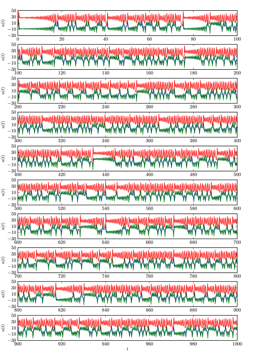
In Figure 2, we plot the solution of the Lorenz system on the interval $[0,1000]$. The solution was computed with $\mathrm{cG}(100)$, which is a method of order $2q=200$, a time step of size $\Delta{}t=0.0037$, 420-digit precision arithmetic, and a tolerance for the discrete residual of size $\epsilon_{\textrm{mach}}\approx 2.26\cdot 10^{-424}$. The very rapid (exponential) accumulation of numerical errors makes the Lorenz “fingerprint” displayed in Figure 2 useful as a reference for verification of solutions of the Lorenz system. If a solution is only slightly wrong, the error is quickly magnified so that the error becomes visible by a direct inspection of a plot of the solution.

Figure 2: Accurate reference solution for the three components of the Lorenz system on the interval $[0,1000]$ with the $x$ and $y$ components plotted in blue and green respectively (and almost overlaid) and the $z$ component in red.

4.1.2 Order of convergence and optimal step size

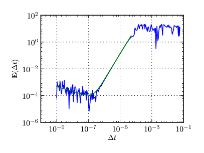
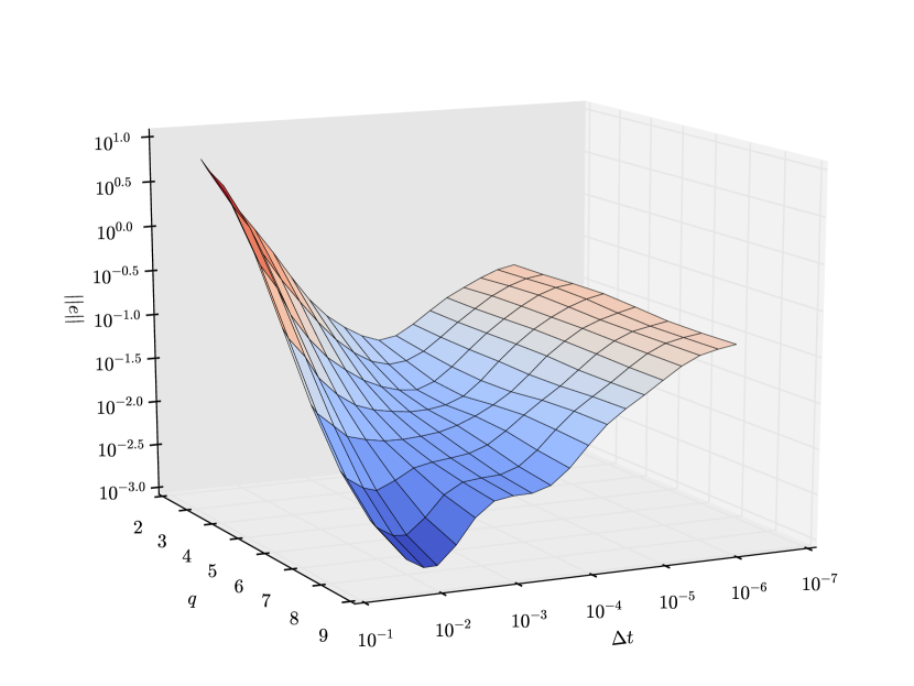
We next investigate how the accumulated error at final time depends on the size of the time step $\Delta{}t$. According to (10), we expect the error to scale like $\Delta{}t^{2q}+\Delta{}t^{-\nicefrac{{1}}{{2}}}\epsilon_{\textrm{mach}}$. Thus, for a gradually decreasing step size, we expect the error to decrease at a rate of $\Delta{}t^{2q}$. However, as the time step becomes smaller the second term $\Delta{}t^{-\nicefrac{{1}}{{2}}}$ will grow and, for small enough $\Delta{}t$, be the dominating contribution to the error. This picture is confirmed by the results presented in Figure 3 for two numerical methods, the $2$nd order $\mathrm{cG}(1)$ and the $10$th order $\mathrm{cG}(5)$ method. Of particular interest in this figure is the very short range in which the $10$th order convergence of the $\mathrm{cG}(5)$ method is recovered; with only 16 digits of precision, the dominating contribution to the total error is the accumulated round-off error. We also note that for both methods, one may find an optimal size of the time step $\Delta{}t$ for which both contributions to the total error are balanced.

Figure 3: Error at time $T=30$ for the $\mathrm{cG}(1)$ solution (left) and at time $T=40$ for the $\mathrm{cG}(5)$ solution (right) of the Lorenz system. The slopes of the green lines are $-0.35\approx-1/2$ and $1.95\approx 2$ for the $\mathrm{cG}(1)$ method. For the $\mathrm{cG}(5)$ method, the slopes are $-0.49\approx-1/2$ and $10.00\approx 10$.

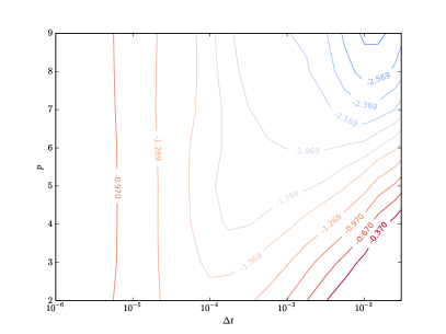
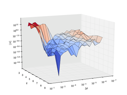
In Figure 4, results are presented for an investigation of the influence on both the step size $\Delta{}t$ and the polynomial degree $q$ in the $\mathrm{cG}(q)$ method. As expected, the minimal error is obtained when both the polynomial degree $q$ and the step size are maximal. Maximising the step size minimizes the influence of numerical round-off errors (the term $\Delta{}t^{-\nicefrac{{1}}{{2}}}$), and as a consequence the polynomial degree $q$ must be large in order to suppress the discretisation error (the term $\Delta{}t^{2q}$).

Figure 4: Top: The accumulated total error at final time $T=40$ for numerical solutions of the Lorenz system with different step size $\Delta{}t$ and polynomial degree $q$ using the $\mathrm{cG}(q)$ method. Due to the random nature of the round-off errors, the data has been smoothed. Lower left: Contour lines of the smoothed data. Lower right: The raw data included for completeness.

4.2 The Van der Pol oscillator

We next consider the Van der Pol oscillator, given by the second order ODE

$$\ddot{u}=\mu(1-u^{2})\dot{u}-u.$$

Rewritten as a system of first order equations, it reads

$$\left\{\begin{aligned} \dot{u}_{1}&=u_{2},\\ \dot{u}_{2}&=\mu(1-u_{1}^{2})u_{2}-u_{1}.\\ \end{aligned}\right.$$ (13)

We compute solutions on $[0,2\mu]$ for $\mu=10^{3}$ and $u(0)=(2,0)$. This configuration is used as a test problem for ODE solvers in Testset2008 . For large values of the parameter $\mu$, the solution quickly approaches a limit cycle.

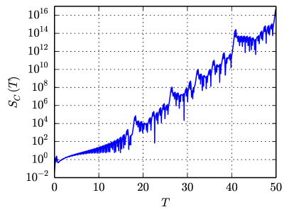
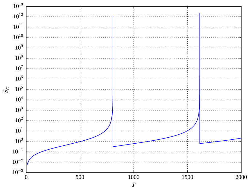
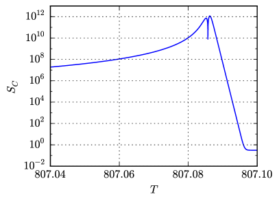
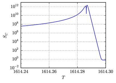
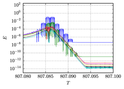
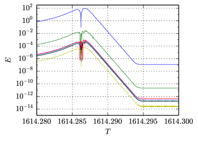
As for the Lorenz system, the stability factors(s) grow very rapidly (exponentially), as indicated in Figures 5 and 6. However, the rapid growth is localised in time close to $T\approx 807\cdot n$ for $n\in\mathbb{N}$. For times before or after these points of instability, the stability factor is of moderate size. This means that solutions are difficult to compute only at points near the points of instability; that is, a solution may be easily computed at time $t=1000$ but not at time $t=807$.

Figure 5: Growth of the computational stability factor $S_{C}(T)$ for the Van der Pol oscillator (13).

Figure 6: Detail of growth of the computational stability factor $S_{C}(T)$ for the Van der Pol oscillator (13).

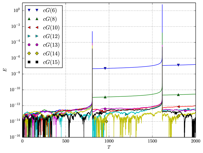
This rapid growth of stability factors is reflected in the growth of the error for numerical solutions as shown in Figures 7 and 8. Examining these plots in more detail, we notice that in accordance with the error estimate of Theorem 3.2 and Equation (10). For the numerical solutions studied in Figures 7 and 8, the discretisation error dominates for low order methods. As the polynomial degree $q$ is increased, the error decreases until the point when the computational error starts to dominate. We notice that the baseline error is of size $E\sim 10^{-14}$ for the highest order methods when the stability factor is of size $S\sim 10^{2}$, and the error spikes at $E\sim 10^{-4}$ at times when the stability factor takes on large values $S\sim 10^{12}$. This is in good agreement with the error estimate: $E\sim S\cdot 10^{-16}$.

Figure 7: Growth of error for solutions of the Van der Pol oscillator (13) computed with time step $\Delta{}t=10^{-3}$.

Figure 8: Detail of growth of error for solutions of the Van der Pol oscillator (13) computed with time step $\Delta{}t=10^{-3}$.

5 Conclusions

We have proved error estimates accounting for data, discretisation and computational (round-off) errors in the numerical solution of initial value problems for ordinary differential equations. These error estimates quantify the accumulation rates for numerical round-off error as inversely proportional to the square root of the step size, and proportional to a specific computable stability factor. The effect of round-off errors is mostly pronounced for large values of the stability factor, which includes both chaotic dynamical systems as well as long-time integration of systems which exhibit only a moderate growth of the stability factor.

References

- (1) Becker, R., Rannacher, R.: An optimal control approach to a posteriori error estimation in finite element methods. Acta Numerica 10, 1––102 (2001)
- (2) Cao, Y., Petzold, L.: A posteriori error estimation and global error control for ordinary differential equations by the adjoint method. SIAM Journal on Scientific Computing 26(2), 359–374 (2004)
- (3) Coomes, B.A., Kocak, H., Palmer, K.J.: Rigorous computational shadowing of orbits of ordinary differential equations. Numerische Mathematik 69(4), 401––421 (1995)
- (4) Delfour, M., Hager, W., Trochu, F.: Discontinuous Galerkin methods for ordinary differential equations. Math. Comp. 36, 455––473 (1981)
- (5) Eriksson, K., Estep, D., Hansbo, P., Johnson, C.: Introduction to adaptive methods for differential equations. Acta Numerica 4, 105––158 (1995)
- (6) Estep, D.: A posteriori error bounds and global error control for approximations of ordinary differential equations. SIAM J. Numer. Anal. 32, 1–48 (1995)
- (7) Estep, D., French, D.: Global error control for the continuous Galerkin finite element method for ordinary differential equations. M2AN 28, 815––852 (1994)
- (8) Estep, D., Johnson, C.: The pointwise computability of the Lorenz system. Math. Models. Meth. Appl. Sci. 8, 1277–1305 (1998)
- (9) Granlund, T., the GMP development team: GNU MP: The GNU Multiple Precision Arithmetic Library (2015). http://gmplib.org/
- (10) Hairer, E., McLachlan, R.I., Razakarivony, A.: Achieving brouwer’s law with implicit runge–kutta methods. BIT Numerical Mathematics 48(2), 231–243 (2008)
- (11) Higham, N.: Accuracy and stability of numerical algorithms, second edn. Society for Industrial Mathematics (2002)
- (12) Hulme, B.L.: Discrete Galerkin and related one-step methods for ordinary differential equations. Math. Comput. 26(120), 881––891 (1972)
- (13) Hulme, B.L.: One-step piecewise polynomial Galerkin methods for initial value problems. Math. Comput. 26(118), 415––426 (1972)
- (14) Johnson, C.: Error estimates and adaptive time-step control for a class of one-step methods for stiff ordinary differential equations. SIAM J. Numer. Anal. 25(4), 908––926 (1988)
- (15) Jorba, A., Zou, M.: A software package for the numerical integration of ODEs by means of high-order Taylor methods. Experimental Mathematics 14(1), 99––117 (2005)
- (16) Kehlet, B.: Analysis and implementation of high-precision finite element methods for ordinary differential equations with application to the Lorenz system. MSc thesis, Department of Informatics, University of Oslo (2010)
- (17) Kehlet, B., Logg, A.: Quantifying the computability of the Lorenz system. In: Adaptive Modeling and Simulation (2013)
- (18) Kehlet, B., Logg, A.: Code package for the paper ”A posteriori error analysis of round-off errors in the numerical solution of ordinary differential equations” (2015). DOI 10.5281/zenodo.16671. URL http://dx.doi.org/10.5281/zenodo.16671. Available at http://dx.doi.org/10.5281/zenodo.16671
- (19) Li, J., Zeng, Q., Chou, J.: Computational uncertainty principle in nonlinear ordinary differential equations i: Numerical results. Science in China (E) 43(5), 449–460 (2000)
- (20) Li, J., Zeng, Q., Chou, J.: Computational uncertainty principle in nonlinear ordinary differential equations ii: Theoretical analysis. Science in China (E) 44(1), 55–74 (2001)
- (21) Logg, A.: Multi-Adaptive Galerkin methods for ODEs I. SIAM J. Sci. Comput. 24(6), 1879––1902 (2003)
- (22) Logg, A.: Multi-Adaptive Galerkin methods for ODEs II: Implementation and applications. SIAM J. Sci. Comput. 25(4), 1119––1141 (2003)
- (23) Logg, A., Kehlet, B.: Tanganyika. https://bitbucket.org/benjamik/tanganyika
- (24) Lorenz, E.N.: Deterministic nonperiodic flow. J. Atmosph. Sci. 20, 130––141 (1963)
- (25) Mazzia, F., Magherini, C.: Test set for initial value problem solvers, release 2.4. Technical Report 4, Department of Mathematics, University of Bari, Italy (2008). Available at http://pitagora.dm.uniba.it/~testset
- (26) Viswanath, D.: The fractal property of the Lorenz attractor. Physica D: Nonlinear Phenomena 190(1-2), 115–128 (2004)