Dynamics of the Density of Quantized Vortex-Lines in Superfluid Turbulence

Abstract

The quantization of vortex lines in superfluids requires the introduction of their density ${\mathcal{L}}({\bm{r}},t)$ in the description of quantum turbulence. The space homogeneous balance equation for ${\mathcal{L}}(t)$, proposed by Vinen on the basis of dimensional and physical considerations, allows a number of competing forms for the production term ${\mathcal{P}}$. Attempts to choose the correct one on the basis of time-dependent homogeneous experiments ended inconclusively. To overcome this difficulty we announce here an approach that employs an inhomogeneous channel flow which is excellently suitable to distinguish the implications of the various possible forms of the desired equation. We demonstrate that the originally selected form which was extensively used in the literature is in strong contradiction with our data. We therefore present a new inhomogeneous equation for ${\mathcal{L}}({\bm{r}},t)$ that is in agreement with our data and propose that it should be considered for further studies of superfluid turbulence.

Background: Below the Bose-Einstein condensation temperature $T_{\lambda}\approx 2.18\,$K, liquid ⁴He becomes a quantum inviscid superfluidb:a ; b:b ; b:Annett ; b:SS-2012 . Aside from the lack of viscosity, the vorticity in ⁴He is constrained to vortex-line singularities of fixed circulation $\kappa=h/M$, where $h$ is Planck’s constant and $M$ is the mass of the ⁴He atom. These vortex lines have a core radius $a_{0}\approx 10^{-8}\,$cm, compatible with the interatomic distance. In generic turbulent states, these vortex lines appear as a complex tangle with a typical intervortex distance $\ell$ nem .

Recent progress in laboratory Helsinki-rev ; b:PNAC2 ; b:PNAC1 ; b:PNAC3 ; b:PNAC4 ; b:11 ; B:12 ; B:13 ; B:14 ; B:15 ; B:19 ; B:20 ; B:21 ; B:22 ; B:23 ; b:17 ; b:18 and numerical studies b:SS-2012 ; b:PNAC2 ; b:PNAC5 ; b:PNAC6 ; B:9 ; b:Kond-1 ; b:PNAC7 ; b:A-10 of superfluid turbulence in superfluid ³He and ⁴He led to a growing consensus that the statistical properties of superfluid turbulence at large scales $R\gg\ell$ are similar to those of classical turbulence. An acceptable theory of these large scale properties LNV-2004 ; LNS-2006 ; LNR-2008 ; BLPP-2012 ; BLPP-2013 ; b:PNAC2 ; b:PNAC1 ; BLNNPP-2015 is based on the Landau-Tisza two-fluid model b:L-41 ; b:T-40 , using ‘normal’ and ‘superfluid’ components of densities $\rho_{\text{n}}$ and $\rho_{\text{s}}$ with velocity fields ${\bm{u}}_{\text{n}}({\bm{r}},t)$ and ${\bm{u}}_{\text{s}}({\bm{r}},t)$. This model was extended by Hall-VinenHV and Bekarevich-KhalatnikovBK to include a mutual friction between the components, proportional to the the vortex-line density ${\mathcal{L}}$. This means that a theory of large-scale motions which is affected by the mutual friction requires the inclusion of the dynamics of ${\mathcal{L}}$.

The situation changes drastically upon considering the statistical properties on smaller scales, where the quantization of vortex lines becomes crucial. Several statistical characteristics of the vortex tangle become essential for a consistent description. Besides ${\mathcal{L}}$, these characteristics involve the mean-square curvature $(\tilde{S})^{2}$, the vortex tangle anisotropy parameters $I_{\parallel}$ and $I_{\ell}$ introduced by Schwarzb:1 . The most important of these is the vortex line density ${\mathcal{L}}({\bm{r}},t)$. It is expected that coupling one or more of these quantities to the variables of the two fluid Hall-Vinen-Bekarevich-Khalatnikov equations HV ; BK is a minimal requirement for an acceptable theory of quantum turbulence.

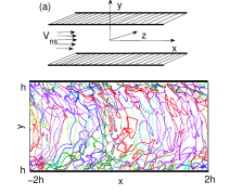
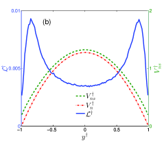
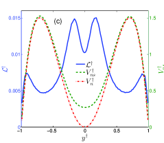
Figure 1: Numerical setup and obtained profiles of counterflow velocity and vortex line density. Panel a: Upper figure: Plane channel flow geometry $L_{x}\times L_{y}\times L_{z}$, $L_{x}=4h,L_{y}=2h,L_{z}=2h,h=0.05$ cm. Lower figure: Projection of a vortex tangle on the $(x,y)$-plane, orthogonal to the walls. Different colors are used to distinguish vortex lines. Panels b and c: Prescribed parabolic (b) and non-parabolic (c) normal velocity profiles $V_{\text{n}}^{\dagger}(y^{\dagger})$ ($-\cdot-$), the resulting counterflow profiles $V_{\text{ns}}^{\dagger}(y^{\dagger})$ ($--$) and the resulting profiles of ${\mathcal{L}}^{\dagger}(y^{\dagger})$ (—) in dimensionless unites defined by Eqs. (8). $T=1.6\;$K.

The problem: A phenomenological equation of motion for ${\mathcal{L}}(t)$ was suggested by Vinen for homogeneous counterflowsb:5 ; b:6 already in 1957:

$${d{\mathcal{L}}(t)}/{dt}={\mathcal{P}}(t)-{\mathcal{D}}(t)\ .$$ (1a)

Here the production term $${\mathcal{P}}(t) {\mathcal{L}} V_{\text{ns}} {\mathcal{D}}(t) V_{\text{ns}} \alpha {\mathcal{L}} {\mathcal{L}} V_{\text{ns}} {\mathcal{P}} {\mathcal{D}} \alpha \kappa V_{\text{ns}} {\mathcal{L}}(t) \widetilde{S} I_{\parallel} I_{\ell}$$ describes the growth of due to the extension of the vortex rings by mutual friction which is caused by the difference between the velocities of the normal and super components (“the counterflow velocity” ). The decay term, is again caused by the mutual friction due to the moving normal fluid components and is assumed to be independent of . Therefore both terms should be proportional to the dimensionless dissipative mutual friction parameter . In principle it is not guaranteed that the equation for can be closed via and . Such a closure for and b:5 assumes that (beside , and ) the only relevant variable in the problem is the instantaneous value , while , , , etc. are to some extent unimportant. Upon accepting this closure idea the dimensional reasoning dictatesb:5 ; b:6 ; nem :

$${\mathcal{P}}\Rightarrow{\mathcal{P}}_{\text{cl}} = \alpha\,\kappa{\mathcal{L}}^{2}F(x)\,,\quad x\equiv V_{\text{ns}}^{2}\big{/}\kappa^{2}{\mathcal{L}}\,,$$ (1b)

$${\mathcal{D}}\Rightarrow{\mathcal{D}}_{\text{cl}} = \alpha\,\kappa{\mathcal{L}}^{2}G(x)\ .$$ (1c)

Here $F(x)$ and $G(x)$ are dimensionless functions of the dimensionless argument $x$.

The most delicate issue in this approach is the determination of the functions $F(x)$ and $G(x)$. Vinenb:5 assumed that the decay term ${\mathcal{D}}$ is independent of ${\bm{V}}_{\text{ns}}$ leading to $G(x)=C_{\rm dec}$. On the other hand Vinen and later authors (see, e.g. b:Kop ) chose ${\mathcal{P}}$ to be proportional to the mutual friction force $f\propto\alpha|V_{\text{ns}}|$, leading to the proposition that $F(x)\propto\sqrt{x}$, and then

$${\mathcal{P}}_{\text{cl}}\Rightarrow{\mathcal{P}}_{1}=\alpha\,C_{1}{\mathcal{L}}^{3/2}|V_{\text{ns}}|\,,$$ (2a)

where $$C_{1} {\mathcal{L}} d{\mathcal{L}}/dt F(x) F(x)\propto x$$ is a dimensionless constant. Vinenb:6 realized that (2a) is not the only possibility. Another choice can follow the spirit of Landau’s theory of critical phenomena, considering as an order parameter which determines via an analytical function . Then the leading term in the expansion of giving:

$${\mathcal{P}}_{\text{cl}}\Rightarrow{\mathcal{P}}_{2}=\alpha\,C_{2}{\mathcal{L}}\,V_{\text{ns}}^{2}\big{/}\kappa\ .$$ (2b)

Both options (2) are of course dimensionally correct and they predict the same stationary solution, $${\mathcal{L}}_{\text{st}}\propto V_{\text{ns}}^{2}$$, which is well supported by both experiments and numerical simulations (see, e.g. b:Kond-1 and references therein).

In principle, one could hope to distinguish between the different forms of this important equation by comparing their prediction for the time evolution from some initial condition toward ${\mathcal{L}}_{\text{st}}$ in the presence of counterflow $V_{\text{ns}}$. Unfortunately, the difference in prediction is too small. Neither Vinen b:6 himself nor later b:8 experimental attempts succeeded to distinguish between these two forms . We have made our own attempts to distinguish between the two discussed models (2) by numerical simulation of space homogeneous counterflow turbulence, finding inconclusive results as well.

The proposed resolution of this old conundrum can be obtained by studying inhomogeneous flows like channel flows in which the various relevant variables have nontrivial profiles. We will argue that in fact none of the equations (2) are correct. We propose yet a third form of ${\mathcal{P}}$ [corresponding to $f(x)\propto x^{3/2}$]:

$${\mathcal{P}}_{\text{cl}}\Rightarrow{\mathcal{P}}_{3}=\alpha\,C_{\text{prod}}\sqrt{{\mathcal{L}}}\,V_{\text{ns}}^{3}\big{/}\kappa^{2}\ .$$ (3a)

Being dimensionally correct this closure fits the data that are presented below significantly better than either of the equations (2). We are led to a revision of the homogeneous equation of motion for the field $${\mathcal{L}}({\bm{r}},t)$$ in the form

$$\frac{\partial{\mathcal{L}}({\bm{r}},t)}{\partial t}+{\bm{\nabla}}\cdot\bm{\mathcal{J}}_{\text{cl}}({\bm{r}},t)={\mathcal{P}}_{3}({\bm{r}},t)-{\mathcal{D}}_{\text{cl}}({\bm{r}},t)\ .$$ (3b)

Here we have added a vortex-line density flux $$\bm{\mathcal{J}}({\bm{r}},t) \bm{\mathcal{J}}({\bm{r}},t)$$. Based on our numerical simulations (see below) we suggest to model as follows:

$$\bm{\mathcal{J}}_{\text{cl}}({\bm{r}},t)=-C_{\text{flux}}\big{(}\alpha\big{/}2\kappa\big{)}{\bm{\nabla}}V_{\text{ns}}^{2}\ .$$ (3c)

Notice that the suggested Eqs. (3) are based on our analysis of counterflow turbulence with laminar normal fluid components. Nevertheless we believe that Eqs. (3) or their modifications may serve as a basis for future studies of inhomogeneous superfluid turbulence in a wide variety of conditions, including the evolution of a neutron-initiated micro big bang in superfluid ³He BB , turbulent counterflows and pressure-driven superfluid channel and pipe flows of ⁴He, turbulent flow of ³He in rotating cryostat Helsinki-rev , etc..

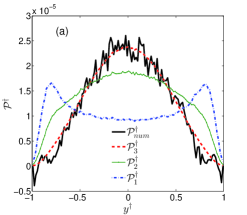
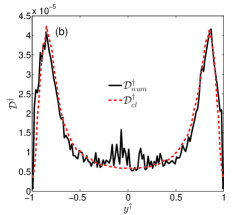
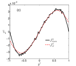
Figure 2: For parabolic normal velocity profile: A comparison between production (${\mathcal{P}}$), decay (${\mathcal{D}}$) and flux (${\mathcal{J}}$) as obtained from numerical simulation and those obtained using their closure versions. Comparison of the numerical data ( -​-) to the competing production forms of the Vinen equation (Panel a): ($-\cdot-$) –${\mathcal{P}}_{1}$, Eq. (2a), (—) – ${\mathcal{P}}_{2}$, Eq. (2b) and ($-~{}-$) – ${\mathcal{P}}_{3}$, Eq. (3b). Comparison of the numerical data for decay (Panel b) and flux term (panel c) with Eq. (1c) for ${\mathcal{D}}$ and Eq. (3c) for ${\mathcal{J}}$ – ($-~{}-$).

Starting from first principles: To reach the desired equation (3b) we denote the coordinates of the quantized vortex lines by ${\bm{s}}(\xi,t)$, which is parameterized by the arc-length $\xi$. Schwarz b:1 derived the equation of motion for the length of the vortex-line segment $\delta\xi$:

$$\frac{1}{\delta\xi}\frac{d\delta\xi}{dt}\approx\alpha{\bm{V}}_{\text{ns}}({\bm{s}},t)\cdot(\bm{s}^{\prime}\times\bm{s}^{\prime\prime})\ .$$ (4a)

Here $$\bm{s}^{\prime}=d\bm{s}/d\xi \bm{s}^{\prime\prime}=d^{2}\bm{s}/d\xi^{2} \alpha {\bm{V}}_{\text{ns}} {\bm{s}} t {\bm{V}}^{\text{n}} {\bm{V}}^{\text{s}}$$, , is the temperature dependent dissipative mutual friction parameter. The counterflow velocity (which is a function of and which we suppress for notational simplicity) is the difference between the normal fluid velocity and super-fluid velocity :

$${\bm{V}}_{\text{ns}}\equiv{\bm{V}}^{\rm n}-\bm{V}^{\rm s}\,,\ {\bm{V}}^{\text{s}}={\bm{V}}^{\text{s}}_{0}+{\bm{V}}_{\scriptscriptstyle\rm{BS}}\ .$$ (4b)

The super-fluid velocity $${\bm{V}}^{\text{s}} {\bm{V}}^{\rm s}_{0} {\bm{V}}_{\scriptscriptstyle\rm{BS}} {\mathcal{C}}$$ includes the macroscopic potential part , and the Biot-Savart velocity . The later term is defined by the entire vortex tangle configuration :

$${{\bm{V}}}_{\scriptscriptstyle\rm{BS}}=\frac{\kappa}{4\pi}\int_{{\mathcal{C}}}\frac{(\bm{s}-\bm{s}_{1})\times\bm{d}s_{1}}{|\bm{s}-\bm{s}_{1}|^{3}}={\bm{V}}^{\text{s}}_{\scriptscriptstyle\rm{LIA}}+{\bm{V}}_{\text{nl}}^{\text{s}}\ .$$ (4c)

The integral (4c) is logarithmically divergent when $${\bm{s}}_{1}\to{\bm{s}} a_{0} R\equiv 1/\widetilde{S} {\bm{V}}_{\scriptscriptstyle\rm{BS}} a_{0} R a_{0}\leqslant|{\bm{s}}_{1}-{\bm{s}}|\leqslant R$$. It is customary to regularize it by using the vortex core radius and the mean vortex line curvature radius . The main contribution to originates from integrating over scales between and , i.e. . This contribution is known as the “Local Induction Approximation” (LIA)b:1 and is written as:

$${\bm{V}}^{\text{s}}_{\scriptscriptstyle\rm{LIA}}=\beta\bm{s}^{\prime}\times\bm{s}^{\prime\prime}\,,\quad\beta\equiv(\kappa/4\pi)\ln\big{(}R/a_{0}\big{)}\ .$$ (4d)

The $${\bm{V}}^{\text{s}}_{\text{nl}} {\mathcal{C}}^{\prime} |{\bm{s}}_{1}-{\bm{s}}|>R$$ term is non-local, being produced by the rest of the vortex configuration, , with :

$${\bm{V}}^{\text{s}}_{\text{nl}} = \frac{\kappa}{4\pi}\int_{{\mathcal{C}}^{\prime}}\frac{(\bm{s}-\bm{s}_{1})\times\bm{d}s_{1}}{|\bm{s}-\bm{s}_{1}|^{3}}\,\ \ .$$ (4e)

The next step is to integrate Eq. (4a) over the vortex tangle in a fixed volume $\Omega$ which resides in slices between $y$ and $y+\delta y$, going over all $x$ and $z$. This provides us with the equation of motion for ${\mathcal{L}}(y,t)\equiv{\int_{{\mathcal{C}}_{\Omega}}d\xi}/{\Omega}$. This equation is written in the form similar to Eq. (3b):

$$\frac{\partial{\mathcal{L}}(y,t)}{\partial t}+\frac{\partial{\mathcal{J}}(y,t)}{\partial y}={\mathcal{P}}(y,t)-{\mathcal{D}}(y,t)\,,$$ (5)

with the following identification for the flux ${\mathcal{J}}$ (toward the walls), production ${\mathcal{P}}$ and decay term ${\mathcal{D}}$:

$${\mathcal{P}}(y,t) = \frac{\alpha}{\Omega}\int_{{\mathcal{C}}_{\Omega}}d\xi\,({\bm{V}}^{\rm n}-{\bm{V}}^{\rm s}_{0}-V_{\rm nl}^{\rm s})\cdot({\bm{s}}^{\prime}\times{\bm{s}}^{\prime\prime})\,,~{}~{}~{}~{}~{}$$ (6a)

$${\mathcal{D}}(y,t) = \frac{\alpha\beta}{\Omega}\int_{{\mathcal{C}}_{\Omega}}d\xi\,|{\bm{s}}^{\prime\prime}|^{2}=\alpha\beta{\mathcal{L}}\widetilde{S}^{2}\,,$$ (6b)

$${\mathcal{J}}(y,t) = \frac{1}{\Omega}\int_{{\mathcal{C}}_{\Omega}}d\xi V_{{\rm drift},y}=\frac{\alpha}{\Omega}\int_{{\mathcal{C}}_{\Omega}}d\xi\,V_{\text{ns,x}}s^{\prime}_{z}\ .$$ (6c)

Here the production and decay terms come directly from integrating Eq. (4a); they coincide with the corresponding equations in Ref.b:1 with the only difference that in Eqs. (6) the integrals are taken in the slice $\Omega$ (between $y$ and $y+\delta y$), while in b:1 the integrals are taken over the entire volume. In the flux term the drift velocity ${\bm{V}}_{\text{drift}}(\xi)$ of the vortex line segment ${\bm{s}}(\xi),$, can be found from the vortex filament equationsb:1 and written as follows:

$${\bm{V}}_{\text{drift}}(\xi)={\bm{V}}^{\text{s}}+\alpha{\bm{s}}^{\prime}\times{\bm{V}}_{\text{ns}}\ .$$ (7)

The mean value of ${\bm{V}}^{\text{s}}$ is oriented along the $x$ direction and it does not contribute to the $y$ component of the flux, ${\mathcal{J}}$. The $y$-component of the second term in Eq. (7) gives the final expression in Eq. (6c).

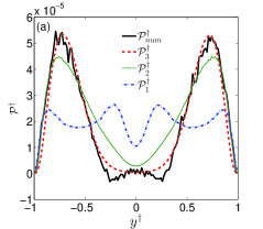
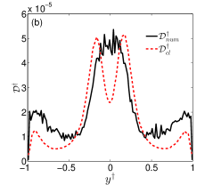
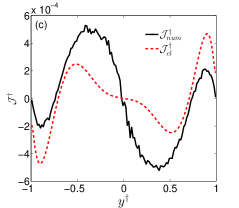
Figure 3: For non-parabolic normal velocity profile: A comparison between production (${\mathcal{P}}$), decay (${\mathcal{D}}$) and flux (${\mathcal{J}}$) as obtained from numerical simulation and those obtained using their closure versions. Comparison of the numerical data ( -​-) to the various allowed production forms of the Vinen equation (Panel a): ($-\cdot-$) –${\mathcal{P}}_{1}$, Eq. (2a), (—) – ${\mathcal{P}}_{2}$, Eq. (2b) and ($-~{}-$) – ${\mathcal{P}}_{3}$, Eq. (3b). Comparison of the numerical data for decay (Panel b) and flux term (panel c) with Eq. (1c) for ${\mathcal{D}}$ and Eq. (3c) for ${\mathcal{J}}$ – ($-~{}-$).

Numerical simulations were set up in a 3-dimensional planar channel geometry (see Fig. 1a) of half-width $h$ with prescribed time-independent profile of the streamwise projection of the normal velocity $V_{x}^{\text{n}}(y)$. To find the vortex tangle configurations we used the vortex filament method, taking into account the potential flow $V_{0}^{\text{s}}$ to maintain the counterflow condition. Details of the simulation method can be found in Refs. b:1 ; b:Kond-1 . Here we used the reconnection method Samuels92 and the line resolution $\Delta\xi=1.6\times 10^{-3}$ cm. Periodic conditions were used in the streamwise and spanwise directions. Taking into account the fact that the boundary conditions for the superfluid component are still under discussion we adopt their simplest version: in the wall-normal $y$ direction $V_{y}^{\text{s}}(\pm h)=0$ and ${\bm{s}^{\prime}(\pm h)}=(0,\pm 1,0)$ at the solid walls. Periodically wrapped replicas of the tangle configuration were used in the $x$- and $z$- directions, with reflected configurations in the $y$ direction.

Having selected a stationary profile of $V_{x}^{\text{n}}(y)\equiv V_{\text{n}}(y)$ we started with a set of arbitrary oriented circular vortex rings and solved the equation for the vortex line evolution. For the obtained dense vortex tangle we found the time-averaged profile $\left\langle V_{x}^{\text{s}}(y)\right\rangle_{t}\equiv V_{\text{s}}(y)$. In all cases we ran the simulations until we obtained steady mean profiles. We take temperature $T=1.6$ K with mutual friction coefficients $\alpha=0.098,\alpha^{\prime}=0.016$, Ref. DB98 .

We begin with a parabolic profile for $V_{\text{n}}(y)$. The profiles of $V_{\text{ns}}(y)$ and ${\mathcal{L}}(y)$ in the dimensionless form:

$$y^{\dagger}\equiv y/L\,,\ V^{\dagger}\equiv V/\sqrt{\left\langle V_{\text{ns}}^{2}\right\rangle}\,,\ {\mathcal{L}}^{\dagger}\equiv\kappa^{2}{\mathcal{L}}/\left\langle V_{\text{ns}}^{2}\right\rangle\,,$$ (8)

are shown in Fig. 1b. Taking integrals in Eqs. (6) over the numerically found vortex tangle configuration we can compute the production, decay and flux terms, denoted as ${\mathcal{P}}_{\text{num}}(y,t)$, ${\mathcal{D}}_{\text{num}}(y,t)$ and ${\mathcal{J}}_{\text{num}}(y,t)$, respectively . Then we compared them with the various their closure versions, ${\mathcal{P}}_{1}$, ${\mathcal{P}}_{2}$, ${\mathcal{P}}_{\text{cl}}$, ${\mathcal{D}}_{\text{cl}}$ and ${\mathcal{J}}_{\text{cl}}$.

From the theoretical point of view the questions are: can we approximate the integrals in Eqs. (6) only in terms of the counterflow velocity $V_{\text{ns}}$ and ${\mathcal{L}}$ itself, or would the integrals produce other dynamical variables that should require further coupled equations to close the system? Is closure possible in general, or only in some conditions?

Assuming that closure is allowed, dimensional considerations presented us with different versions for the production term ${\mathcal{P}}_{n}(y)$ given by Eqs. (2a), (2b) and (3a) for $n=1,2$ and 3. With the widely accepted approximation b:1 that the tangle curvature radius $R=1/\widetilde{S}$ is proportional to the intervortex distance $\ell=1/\sqrt{{\mathcal{L}}}$  one gets from Eqs. (6b) and (4d) the closure (1c) for ${\mathcal{D}}$ with

$$C_{\text{dec}}=c_{2}^{2}\ln(R/a_{0})/4\pi\,,\quad\mbox{where}\ c_{2}\equiv\ell\widetilde{S}\ .$$ (9)

For the flux term (3c) we suggest (in the channel geometry):

$${\mathcal{J}}_{\text{cl}}(y,t)=-(\alpha/2\kappa)\,C_{\text{flux}}\partial\,V_{\text{ns}}^{2}/\partial y\ .$$ (10)

In Fig. 2 we compare the numerical integrals (6) (shown as thick solid black lines) with corresponding closures. The dot-dashed blue line in Fig. 2a shows the Vinen prediction, ${\mathcal{P}}_{1}(y)$, (2a), while the thin solid green line shows the alternative form ${\mathcal{P}}_{2}(y)$, Eq. (2b). By dashed red line we show the prediction ${\mathcal{P}}_{\text{3}}(y)$,which is evidently superior to the other two. From this data we can conclude that Eq. (3b) is the one that should be used in the present inhomogeneous case.

Figure 2b shows that the numerical integral (6a) and the commonly used form (1c) for the decay term, ${\mathcal{D}}$, practically coincide, meaning that $c_{2}$, defined by Eq. (9), is indeed $y$-independent. Figure 2c also demonstrates very good agreement between ${\mathcal{J}}_{\text{num}}(y)$ and ${\mathcal{J}}_{\text{cl}}(y)$ given by Eqs. (6c) and (10).

	$V_{\text{n}}$	$\sqrt{\left\langle V_{\text{ns}}^{2}\right\rangle}/V_{\text{n}}$	$C_{\rm prod}$	$C_{\text{dec}}$	$C_{\text{flux}}$	$C_{\text{dec}}\left\langle V_{\text{ns}}^{2}\right\rangle$	$C_{\text{flux}}/\left\langle V_{\text{ns}}^{2}\right\rangle$
	cm/s					(cm/s)2	(s/cm)2
1	1.0	0.788	0.018	6.9	0.088	4.31	0.145
2	1.2	0.785	0.018	4.9	0.124	4.35	0.147
3	1.5	0.780	0.019	3.2	0.210	4.32	0.146
4	1	1.247	0.022	2.3	0.048	3.62	0.039

Table 1: Closure constants for different values of the normal velocity maximum $V_{\text{n}}$ for parabolic (lines 1-3) and non-parabolic (line 4) profiles.

Realizing that the good match between the numerical data and Eq. (3b) may be accidental due to particulary chosen numerical parameters we repeated the simulations with other magnitudes of the counterflow velocities. We found again a good agreement between the numerical profiles ${\mathcal{P}}_{\text{num}}(y)$, ${\mathcal{P}}_{\text{num}}(y)$ and ${\mathcal{J}}_{\text{num}}(y)$ with the corresponding closures, ${\mathcal{P}}_{3}(y)$, ${\mathcal{D}}_{\text{cl}}(y)$ and ${\mathcal{J}}_{\text{cl}}(y)$. Consistency requires that the numerical constants $C_{\text{prod}}$, $C_{\text{dec}}$ and $C_{\text{flux}}$ in these closures should be $V_{\text{ns}}$ independent. Table  1 shows that this is the case only for $C_{\text{prod}}$, while $C_{\text{dec}}$ and $C_{\text{flux}}$ approximately depend on $V_{\text{ns}}$ as: $C_{\text{dec}}\propto 1/\left\langle V_{\text{ns}}^{2}\right\rangle$ and $C_{\text{flux}}\propto\left\langle V_{\text{ns}}^{2}\right\rangle$, where $\left\langle V_{\text{ns}}^{2}\right\rangle$ is the mean-square of $V_{\text{ns}}$ across the channel (which, in its turn $\propto V_{\text{n}}^{2}$). From these facts we can conclude that our closure (3a) for the production term is confirmed, while the traditional closure (1c) for the decay term and simple closure (10) seems to be questionable, although they reproduce well the profiles ${\mathcal{D}}_{\text{num}}(y)$ and ${\mathcal{J}}_{\text{num}}(y)$ in the parabolic case.

To clarify further the quality of the discussed closures we imposed non-parabolic normal velocity profile with two maxima and zero on the centerline, shown in Fig. 1c. Although this profile looks strange, it may be realized in a counterflow experiment with non-homogeneous heating in short enough channel private:S . For this profile we again computed the counterflow and vortex-line density profiles shown in Fig. 1c. Next, we repeated all the steps described before, and found again that our proposed form Eq. (3b) fits the data much better than the other two forms as seen in Fig. 3a. Figures 3b,c show that the closures for the decay and the flux terms, ${\mathcal{D}}_{\text{cl}}$ and $J_{\text{cl}}$, are running into trouble reflecting the numerical profiles only very roughly. In particular this means that $c_{2}^{2}\equiv(\ell\widetilde{S})^{2}$, which is involved in the closure (1c) via Eq. (9), varies across the channel by a factor of three, as follows from Fig. 3b. Recall, that in the parabolic case $c_{2}^{2}$ is $y$-independent, although it depends on $\left\langle V_{\text{ns}}^{2}\right\rangle$ approximately as $1/\left\langle V_{\text{ns}}^{2}\right\rangle$. Consequently, to improve the closure for the decay term one needs to involve an additional balance equation for the tangle curvature $\widetilde{S}$. Similarly, our analysis shows that to improve the closure for the flux term, one needs to involve information about the tangle anisotropy.

Conclusion: The suggested closure (3a) for the production ${\mathcal{P}}_{\text{prod}}(y)$ using the counterflow velocity and the vortex line density profiles can be considered as highly promising. However, the closures for the decay and flux are sensitive, and they may require accounting for additional tangle characteristics. The first candidate is the tangle curvature; the tangle anisotropy also can be important. Much more work in this direction is required to develop a consistent theory of the wall-bounded superfluid turbulence.

This paper had been supported in part by Grant No. 14-29-00093 from Russian Science Foundation. L.K. acknowledges the kind hospitality at the Weizmann Institute of Science during the main part of the project.

References

- (1) R. J. Donnelly, Quantized Vortices in Hellium II (Cambridge Univ. Press, Cambridge, UK, 1991).
- (2) Quantized Vortex Dynamics and Superfluid Turbulence, ed. by C. F. Barenghi et al., Lecture Notes in Physics 571 (Springer-Verlag, Berlin, 2001).
- (3) A. F. Annett, Superconductivity, Superfluids and Condensates (Oxford University Press, Oxford, 2004).
- (4) L. Skrbek, K. R. Sreenivasan, Developed quantum turbulence and its decay, Phys. Fluids 24 011301(2012).
- (5) S. K. Nemirovskii, Quantum turbulence: Theoretical and numerical problems, Phys. Rep. 524, 85 (2013).
- (6) C. F. Barenghi, V. S. L’vov and P.-E. Roche, Experimental, numerical, and analytical velocity spectra in turbulent quantum fluid, Proc. Natl. Acad. Sci. USA 111, (Supl.1), 4683 (2014).
- (7) C. F. Barenghi, L. Skrbek and K. R. Sreenivasan, Introduction to quantum turbulence, Proc. Natl. Acad. Sci. USA 111, (Supl.1), 4647 (2014).
- (8) V.B. Eltsov, R. de Graaf, R. Hanninen, M. Krusius, R.E. Solntsev, V.S. L’vov, A.I. Golov, P.M. Walmsley, Turbulent dynamics in rotating helium superfluids, Progress in Low Temperature Physics, XVI pp. 46-146 (2009).
- (9) E. Fonda, D. P. Meichle, N. T. Ouellette, S. Hormoz, and D. P. Lathrop, Direct observation of Kelvin waves excited by quantized vortex reconnection, Proc. Natl. Acad. Sci. USA 111, (Supl.1), 4707 (2014).
- (10) W. Guo, M. La Mantiac, D. P. Lathrop and S.W. Van Sciver, Visualization of two-fluid flows of superfluid helium-4, Proc. Natl. Acad. Sci. USA 111, (Supl.1), 4653 (2014).
- (11) L. Skrbek, A.V. Gordeev, F. Soukup, Decay of counterflow He II turbulence in a finite channel: Possibility of missing links between classical and quantum turbulence, Phys. Rev. E 67, 047302 (2003).
- (12) S.W. Van Sciver, S. Fuzier, and T. Xu, J., Particle Image Velocimetry Studies of Counterflow Heat Transport in Superfluid Helium II, J. Low Temp. Phys. 148, 225 (2007).
- (13) T. Zhang and S. W. Van Sciver, Large-scale turbulent flow around a cylinder in counterflow superfluid 4He (He (II)), Nat. Phys. 1, 36 (2005).
- (14) G. P. Bewley, D. P. Lathrop, and K. R. Sreenivasan, Superfluid Helium: Visualization of quantized vortices, Nature (London) 441, 588 (2006).
- (15) M. S. Paoletti, R. B. Fiorito, K. R. Sreenivasan, and D. P. Lathrop,Visualization of Superfluid Helium Flow, J. Phys. Soc. Jap. 77, 111007 (2008).
- (16) D. N. McKinsey, W. H. Lippincott, J. A. Nikkel, and W. G. Rellergert, Trace Detection of Metastable Helium Molecules in Superfluid Helium by Laser-Induced Fluorescence, Phys. Rev. Lett. 95, 111101 (2005).
- (17) W. G. Rellergert, S. B. Cahn, A. Garvan, J. C. Hanson, W. H. Lippincott, J. A. Nikkel, and D. N. McKinsey, Detection and Imaging of He2 Molecules in Superfluid Helium, Phys. Rev. Lett. 100, 025301 (2008).
- (18) W. Guo, J. D. Wright, S. B. Cahn, J. A. Nikkel, and D. N. McKinsey, Metastable Helium Molecules as Tracers in Superfluid He4, Phys. Rev. Lett. 102, 235301 (2009).
- (19) W. Guo, S. B. Cahn, J. A. Nikkel, W. F. Vinen, and D. N. McKinsey, Visualization Study of Counterflow in Superfluid He4 using Metastable Helium Molecules Phys. Rev. Lett. 105, 045301 (2010).
- (20) A. Marakov, J. Gao, W. Guo, S. W. Van Sciver, G. G. Ihas, D. N. McKinsey, and W. F. Vinen, Visualization of the normal-fluid turbulence in counterflowing superfluid He4. Phys. Rev. B 91, 094503 (2015).
- (21) C.F. Barenghi, A.V. Gordeev, L. Skrbek, Depolarization of decaying counterflow turbulence in He II, Phys. Rev. E 74, 026309 (2006).
- (22) M. Sciacca, Y.A. Sergeev, C.F. Barenghi, L. Skrbek, Saturation of decaying counterflow turbulence in helium II, Phys. Rev. B 82, 134531 (2010).
- (23) N. G. Berloff, M. Brachet and N. P. Proukakis, Modeling quantum fluid dynamics at nonzero temperatures, Proc. Natl. Acad. Sci. USA 111, (Supl.1), 4675 (2014).
- (24) R. Hänninen and A. W. Baggaley, Vortex filament method as a tool for computational visualization of quantum turbulence, Proc. Natl Acad. Sci. USA 111, (Supl.1), 4667 (2014).
- (25) A. W. Baggaley and Laizet, Vortex line density in counterflowing He II with laminar and turbulent normal fluid velocity profiles, Phys. Fluids 25, 115101 (2013).
- (26) L. Kondaurova, V. L’vov, A. Pomyalov and I. Procaccia, Structure of a quantum vortex tangle in 4He counterflow turbulence, Phys. Rev. B 89, 014502 (2014).
- (27) G. V. Kolmakov, P. V. E. McClintock and S. V. Nazarenko, Wave turbulence in quantum fluids, Proc. Natl. Acad. Sci. USA 111, (Supl.1), 4727 (2014).
- (28) H. Adachi, S. Fujiyama, M. Tsubota, Steady-state counterflow quantum turbulence: Simulation of vortex filaments using the full Biot-Savart law, Phys. Rev. B 81, 104511 (2010).
- (29) V. S. L’vov, S. V. Nazarenko and G. E. Volovik, Energy spectra of developed superfluid turbulence, J. Low Temp. Phys. 80, 535 (2004).
- (30) V.S. L’vov, S.V. Nazarenko and L. Skrbek, Energy Spectra of Developed Turbulence in Helium Superfluids, J. Low Temp. Phys. 145, 125 (2006).
- (31) V. S. L’vov, S. V. Nazarenko and O. Rudenko, Gradual eddy-wave crossover in Superfluid turbulence, J. of Low Temp. Phys. 153, 140-161 (2008).
- (32) L. Boue, V.S. L’vov, A. Pomyalov, I. Procaccia, Energy spectra of superfluid turbulence in He-3B, Phys. Rev. B 85, 104502 (2012).
- (33) L. Boue, V.S. L’vov, A. Pomyalov, I. Procaccia, Enhancement of intermittency in superfluid turbulence, Phys. Rev. Lett., 110, 014502 (2013).
- (34) L. Boue, V S. L’vov, Y. Nagar, S. V. Nazarenko, A. Pomyalov, and I. Procaccia, Energy and Vorticity Spectra in Turbulent Superfluid 4He from T = 0 to Tλ, Phys. Rev. B 91, 144501 (2015).
- (35) L.D. Landau, Theory of superfluidity of helium-II, J. Phys. USSR 5, 71 (1941).
- (36) L. Tisza, J. Phys. Radium 1, 164 (1940) , ibid 1, 350 (1940).
- (37) H.E. Hall, W.F. Vinen, The rotation of liquid helium II. II. The theory of mutual friction in uniformly rotating helium II, Proc. R. Soc. Lond. A Math Phys. Sci. 238, 215 (1956).
- (38) I.L. Bekarevich, I.M. Khalatnikov, Phenomenological Derivation of the Equations of Vortex Motion in He II, Zh. Eksp. Teor. Fiz. 40, 920 (1961) (Sov. Phys. JETP 13, 643 (1961)).
- (39) K.W. Schwarz, Three-dimensional vortex dynamics in superfluid 4He: Homogeneous superfluid turbulence, Phys. Rev. B 38, 2398 (1988).
- (40) W. F. Vinen, Mutual friction in a heat current in liquid helium II. I. Experiments on steady heat currents, Proc. R. Soc. Lond. A Math. Phys. Sci. 240, 114 (1957).
- (41) N. B. Kopnin. Vortex Instability and the Onset of Superfluid Turbulence Phys. Rev. Lett. 92, 135301 (2004).
- (42) W. F. Vinen, Mutual friction in a heat current in liquid helium II. II. Experiments on transient, Proc. R. Soc. Lond. A Math. Phys. Sci. 240, 128 (1957).
- (43) S. K. Nemirovskii and W. Fiszdon, Chaotic quantized vortices and hydrodynamic processes in superfluid helium, Rev. Mod. Phys. 67, 37 (1995).
- (44) Y.M. Bunkov, A. I. Golov, V. S. L’vov, A. Pomyalov and I. Procaccia, Evolution of Neutron-Initiated Micro-Big-Bang in superfluid He 3B, Phys. Rev B 90, 024508 (2014).
- (45) D. C. Samuels , Velocity matching and Poiseuille pipe flow of superfluid helium, Phys. Rev. B 46, 11714 (1992).
- (46) R. J. Donnelly , C. F. Barenghi , The Observed Properties of Liquid Helium at the Saturated Vapor Pressure, J. Phys. Chem. Ref. Data 27, 1217(1998).
- (47) Skrbek, L., private communication.