A Scheduling Model of Battery-powered Embedded System

Abstract

Fundamental theory on battery-powered cyber-physical systems (CPS) calls for dynamic models that are able to describe and predict the status of processors and batteries at any given time. We believe that the idealized system of single processor powered by single battery (SPSB) can be viewed as a generic case for the modeling effort. This paper introduces a dynamic model for multiple aperiodic tasks on a SPSB system under a scheduling algorithm that resembles the rate monotonic scheduling (RMS) within finite time windows. The model contains two major modules. The first module is an online battery capacity model based on the Rakhmatov-Vrudhula-Wallach (RVW) model. This module provides predictions of remaining battery capacity based on the knowledge of the battery discharging current. The second module is a dynamical scheduling model that can predict the scheduled behavior of tasks within any finite time window, without the need to store all past information about each task before the starting time of the finite time window. The module provides a complete analytical description of the relationship among tasks and it delineates all possible modes of the processor utilization as square-wave functions of time. The two modules i.e. the scheduling model and the battery model are integrated to obtain a hybrid scheduling model that describes the dynamic behaviors of the SPSB system. Our effort may have demonstrated that through dynamic modeling, different components of CPS may be integrated under a unified theoretical framework centered around hybrid systems theory.

I Introduction

Modern society is characterized by the pervasive applications of embedded computing systems powered by batteries. Use of batteries endows computing systems with mobility that is appreciated by consumers, industries and governments. Cell phones, portable music/video players, and unmanned airplanes flying over a battle zone are among the most noticeable applications. Computing systems supported by batteries are usually designed following specialized guidelines to reduce power consumption, achieving lower maintenance and longer operation time.

Despite of the great achievements in battery-powered computing, better theoretical understandings of the interactions between computing systems and batteries will be appreciated by applications where power is very limited or battery life is a dominant constraint on systems design. One such application is in underwater robotics, where missions may last more than a year. Although appear to be simple, batteries are complex physical-chemical systems. Hence fundamental research in battery powered embedded computing systems may be viewed as part of the evolving cyber-physical systems (CPS) theory (c.f. recent publications [1, 2, 3, 4, 5, 6]) that aims to develop novel foundations to understand complex physical systems controlled by modern computers.

The complexity of battery discharging behaviors is noticed in literature e.g. [7, 8]. Battery modeling aims to simulate these behaviors by computational models [9, 10]. To support theoretical cyber-physical systems design, a class of analytical models are desired. This is because comparing to physical [11], empirical [12], and circuit based [13, 14] models, analytical models are theoretically tractable while providing sufficient accuracy.

The interactions between batteries and computing systems have been studied by some researchers. Power consumption of computing devices is proportional to $V^{2}_{\rm DD}$ [15], hence can be reduced by dynamic voltage scaling (DVS). Yao et al. [16] propose one of the first DVS-aware scheduling algorithms. Rowe et. al. [17] proposed a scheduling method to combine idle period of tasks so that the processor can be put to sleep to save power. Some recent results on power management in sensor network applications are presented by Ren et. al. [18]. In these works the behaviors of batteries are simplified as ideal voltage sources whose life only depends on the average discharge current. The approach taken by Jiong et. al. [19, 20] uses an empirical battery model and assumes known battery discharge profiles for computing tasks.

We believe that a dynamic model needs to be established that is able to predict battery capacity based on the discharge current determined by a feedback control law or feedback scheduling algorithm. The magnitude and pulse width of such discharge current can not be determined beforehand. Therefore, in previous work [21], we introduce a dynamic battery model that describes the variations of the capacity of a battery under time varying discharge current. This model is input-output equivalent to the Rakhmatov-Vrudhula-Wallach (RVW) model proposed by Rakhmatov et. al. [22] which has been shown to agree with experimental results and has demonstrated high accuracy in battery capacity prediction and battery life estimation. Besides the accuracy, the RVW model is also simple to use. It can characterize any general battery with only two parameters $\alpha$ and $\beta$, which can be estimated by a experimental method introduced in [22]. However, the application of the RVW model requires that the discharge current, as a function of time, is known. Our dynamic model allows battery capacity prediction for feedback control laws and online scheduling algorithms.

This paper is inspired by the need to completely describe the possible battery discharge profiles for a processor that is running a finite number of aperiodic real-time tasks. Knowing such a discharge profile allows us to predict remaining battery capacity at any given moment without seeking the help from simulation programs. We found that the problem can only be solved by establishing a dynamic model that integrates both battery models and task scheduling models. However, we are unable to find existing models from the literature that fits in such requirements.

Therefore, we start our modeling effort by considering a single processor single battery (SPSB) model. This model may appear naive. However, we find it is very challenging to establish a complete analytical description for the behaviors of multiple tasks. Readers in doubt about this difficulty may consider giving an explicit mathematical formula for the processor utilization plots generated by real-time systems simulation tools such as the TrueTime [23]. Such difficulty has been mostly avoided by the works on schedulability [24, 25, 26] because only the worst case scenario, which are the critical time instances, are considered.

With the help from hybrid systems theory evolving in the control community [27, 28], we obtain a class of hybrid dynamical systems models that are able to describe the battery discharge profile when multiple independent aperiodic tasks are scheduled under a fixed priority scheduling algorithm on a single processor. When integrated with the dynamic battery model, theoretical predictions of battery capacity for an SPSB system can be produced online at any given time. Comparing to the literature reviewed, we believe our contribution is novel and may provide foundation for developing novel battery aware scheduling for cyber-physical systems.

The paper is organized as follows. Section III describes the SPSB system we investigate. Section II introduces a dynamic battery model that is used to determine the remaining battery capacity. Section IV derives the dynamic models for two aperiodic tasks on a single processor. The dynamic model also enables us to find analytic descriptions of the processor utilization waveforms in Section V. Section VI extend the conclusion of two tasks to multiple tasks. The models are verified and demonstrated by simulations in Section VII. Conclusions are provided in Section VIII.

II A Dynamic Battery Model

In this section, we briefly review the dynamic battery model established in our recent work [21] as a workshop paper. We model the discharge dynamics within one discharge cycle of (possibly rechargeable) batteries. The discharge cycle starts when a battery is fully charged and ends when the battery can not support the demand for discharge current; no recharging is allowed during the cycle. According to battery and VLSI design literature e.g. [7, 8], the discharge current is supported by the change of concentration of electrolytes near the electrodes of a battery. When the concentration at the electrodes drops below a certain threshold, a battery fails to support discharge current, causing failure to devices it supports. At this moment, the discharge cycle has to stop and the battery needs to be recharged or replaced. Note that there may be a significant amount of electrolytes left when a discharge cycle ends. When the battery is discharged under a pulsed discharge current, during the idle time when current is interrupted, the diffusion process increases electrolyte concentration at the electrodes. This produces the recovery effect that makes the battery appears to have regained portions of its capacity.

The Rakhmatov-Vrudhula-Wallach (RVW) model in [22] is derived from solving the diffusion equations governing the electrolytes motion within a battery. The model captures the recovery effect effectively. As mentioned in the introduction, in order to use the RVW model for CPS design, we derived a dynamic model that is input-output equivalent to the RVW model. The key improvement is to introduce a set of state variables, denoted by ${\bf x}=[x_{0},x_{1},...,x_{m}]$ where $m$ is chosen according to accuracy requirement. In most cases, $m\leq 10$ is accurate enough. Then the dynamic model is given by a linear system:

$$\dot{\bf x} = A{\bf x}+{\bf b}i(t)$$ (1)

$$y = {\bf c}^{\prime}{\bf x}.$$ (2)

Here, the matrix $A$ is a diagonal matrix i.e. $A={\rm diag}\{0,-\lambda_{1},...,-\lambda_{m}\}$ where $\lambda_{j}=\beta*j^{2}$ for $j=1,2,...,m$. The input $i(t)>0$ is the discharge current. The vector ${\bf b}=\frac{1}{\alpha}[1,2,2,...,2]^{\prime}$ and the vector ${\bf c}=[1,1,1,...,1]^{\prime}$. As mentioned in the introduction, $\alpha$ and $\beta$ characterize a battery and they can be estimated by the experimental method introduced in [22]. The output variable $y$ measures the total capacity loss for a battery. It contains two parts, the permanent capacity loss represented by $x_{0}$, and the temporary capacity loss measured by $x_{1},x_{2},...,x_{m}$. At the beginning of the discharge cycle the initial condition for ${\bf x}$ is the zero vector, hence $y=0$. When $y=1$, the discharge cycle ends. The first state variable $x_{0}$ is the integration of the discharge current $i(t)$, hence is the effective discharge delivered to the circuits outside the battery. One can see that the actual discharge $y$ contains more than $x_{0}$. The states $x_{1},x_{2},...,x_{m}$ are temporary capacity losses that are always positive since $i(t)\geq 0$. Under an impulsive current, when $i(t)=0$, $x_{j}(1\leq j\leq m)$ decreases because $-\lambda_{j}<0$. This captures the recovery effect. More details about this model and results regarding optimal discharge profiles are presented in our work [21].

III Scheduled Behaviors of Aperiodic Tasks

In this paper, we consider the case where aperiodic tasks with hard deadlines scheduled on a SPSB system. Tasks are scheduled using the following scheduling algorithm: the tasks with shorter request intervals are assigned higher priorities, and the higher priority tasks can preempt the lower priority tasks. We are interested in the scheduled behaviors of $\tau_{1},...,\tau_{N}$ within a finite time window, which starts from $t_{0}$ with length $L$. $t_{0}$ can be any time instant. Since the request intervals of aperiodic tasks are not constant, the priority assignments among aperiodic tasks may change during the finite time window. To avoid such cases, we enforce the following assumptions on the length of time window $L$.

Assumption III.1

Within $[t_{0},t_{0}+L]$, the maximum request interval of $\tau_{i}$ is smaller than the minimal request interval of $\tau_{i+1}$, where $i$ is selected such that the priority of $\tau_{i}$ is always higher than the priority of $\tau_{i+1}$.

When $t_{0}$ changes, the length of time window and the priority assignments may change as well.

Assumption III.2

We assume that for any time instant $t$, there exists $t_{0}$ and $L$ such that Assumption III.1 is satisfied.

Assumption III.1 guarantees coherence in priority assignments during the finite time window starting from $t_{0}$. Assumption III.2 guarantees that there is no gap between the proper time windows. It is of course trivial to see that periodic tasks satisfy these assumptions within $[t_{0},t_{0}+L]$. In fact, the scheduling algorithm becomes the Rate Monotonic Scheduling (RMS) when the time window $L$ goes to infinity. Our main goal here is to model the behaviors of the tasks, not proposing a new scheduling algorithm.

Since such an modeling effort has not been performed in previous literature, we need to introduce new notations that depict the task behaviors. Suppose $\tau_{\alpha}$ is an independent aperiodic task. We use $t_{\alpha}(n)$ to denote the request time of the $n$-th instance of $\tau_{\alpha}$; $C_{\alpha}(n)$ to denote the computing time of the $n$-th instance of $\tau_{\alpha}$; and $T_{\alpha}(n)$ to denote the request interval of the $n$-th instance of $\tau_{\alpha}$, which is defined to be the interval between the request time of the $n$-th instance of $\tau_{\alpha}$, and the request time of the $(n+1)$-th instance of $\tau_{\alpha}$, i.e. we have $T_{\alpha}(n)=t_{\alpha}(n+1)-t_{\alpha}(n)$.

Regardless of the choice of $t_{0}$, the scheduled behaviors of $\tau_{1},...,\tau_{N}$ within $[t_{0},t_{0}+L]$ is affected by both the tasks requested within $[t_{0},t_{0}+L]$ and the tasks requested before $t_{0}$. To predict the scheduled behaviors within $[t_{0},t_{0}+L]$ by real-time simulation tools such as Truetime, we have to know all task information within $[0,t_{0}+L]$ and simulate from time $0$. However, keeping all task information is costly in the real application and simulating from the beginning is time inefficient. We discover that this problem can be solved by using a dynamical model, instead of storing a large amount of data, we just need to update the value of some state variables. Furthermore, the dynamic model is able to determine the state of the processor at any given time within $[t_{0},t_{0}+L]$.

We develop a recursive algorithm to determine the state of the processor for multiple aperiodic tasks. Our goal is to find out when the processor is occupied within $[t_{0},t_{0}+L]$. The result is a function of time $\Phi:t\to\{0,1\}$ where for $t\in[t_{0},t_{0}+L]$, $\Phi(t)=0$ if the processor is free, and $\Phi(t)=1$ if the processor is busy.

Furthermore, we assume that when $\Phi(t)=1$, a constant current will be drawn from the battery and when $\Phi(t)=0$, the current vanishes. For simplicity, we ignore the possible power difference among tasks and the transients in the battery discharge current. If $\Phi(t)$ is known, we are able to describe the current $i(t)$ drawn from the battery by the processor. And then, using the dynamic battery model, we are able to predict the remaining battery capacity.

IV A Dynamic Scheduling Model for Two Tasks

In this section, we establish a dynamic model for the scheduled behaviors of two independent aperiodic tasks on a single processor within $[t_{0},t_{0}+L]$. Later in this paper, we will develop a recursive algorithm to extend the model to multiple tasks. Consider two tasks $\tau_{\alpha}$ and $\tau_{\beta}$, where $\alpha=1$ and $\beta=2$, scheduled under the scheduling algorithm introduced in Section III. Suppose Assumptions III.1 and III.2 are satisfied, we have the following claim:

Claim 1: $\tau_{\alpha}$ is assigned higher priority than $\tau_{\beta}$ within $[t_{0},t_{0}+L]$.

There is at most one instance of $\tau_{\beta}$ requested within each request interval of $\tau_{\alpha}$.

We determine a set of ”state variables” that completely determine the scheduled behavior of $\tau_{\alpha}$ and $\tau_{\beta}$ at any given time within $[t_{0},t_{0}+L]$. Then transition rules between these states from the current time to all future times are described by a set of nonlinear difference equations.The work presented in this section centered around these two themes—states and transition rules.

IV-A Exploring Task Relationship

In this subsection, we model the dynamics for the request time of $\tau_{\alpha}$ and $\tau_{\beta}$, and explore task relationship between $\tau_{\alpha}$ and $\tau_{\beta}$.

We first select the request time of $\tau_{\alpha}$ and $\tau_{\beta}$ as two state variables. Within the finite time window, $t_{\alpha}(n)$ and $t_{\beta}(m)$ satisfies the following equations

$$\left\{\begin{array}[]{l}t_{\alpha}(n+1)=t_{\alpha}(n)+T_{\alpha}(n)\\ t_{\beta}(m+1)=t_{\beta}(m)+T_{\beta}(m)\end{array}\right.$$ (3)

where $n$ and $m$ are the index numbers for the instances of $\tau_{\alpha}$ and $\tau_{\beta}$ requested within the finite time window. For example, if $\tau_{\alpha}$ has a fixed period, $n$ ranges from $1$ to $\lfloor L/T_{1}\rfloor$ where $T_{1}$ is the period for $\tau_{\alpha}$; and if $\tau_{\beta}$ has a fixed period $T_{2}$, $m$ ranges from $1$ to $\lfloor L/T_{2}\rfloor$.

Next, we explore task relationship between $\tau_{\alpha}$ and $\tau_{\beta}$ by introducing another two state variables $y(n)$ and $z(n)$ . $y(n)$ helps describe the request time of the first instance of $\tau_{\beta}$ requested after the $n$-th instance of $\tau_{\alpha}$, which is denoted by $t_{\beta}(y(n))$. The value of $y(n)$ indicates the index numbers for the instances of $\tau_{\beta}$ requested within the finite time window. If $\tau_{\beta}$ has fixed period $T_{2}$, then $y(n)$ ranges from $1$ to $\lfloor L/T_{2}\rfloor$. $z(n)$ describes the phase difference between the request time of the $n$-th instance of $\tau_{\alpha}$, and the request time of the $y(n)$-th instance of $\tau_{\beta}$, i.e.

$$z(n)=t_{\beta}(y(n))-t_{\alpha}(n).$$ (4)

To determine the transition rules for $y(n)$ and $z(n)$ from $n$ to $n+1$, we need to consider two cases.

Case 1 This case happens when the phase difference satisfies

$$0\leq z(n)<T_{\alpha}(n)$$ (5)

In this case, the $y(n)$-th instance of $\tau_{\beta}$ is requested within $[t_{\alpha}(n),t_{\alpha}(n+1)]$. Thus, the $y(n)$-th instance of $\tau_{\beta}$ is the last instance of $\tau_{\beta}$ requested before $t_{\alpha}(n+1)$. On the other hand, since $y(n+1)$ is defined to be the index number for the first instance of $\tau_{\beta}$ requested after $t_{\alpha}(n+1)$, the $\{y(n+1)-1\}$-th instance of $\tau_{\beta}$ is also the last instance of $\tau_{\beta}$ requested before $t_{\alpha}(n+1)$. Therefore, we have

$$y(n+1)-1=y(n)$$ (6)

In this case, $z(n)$ will update in the following ways

$$z(n+1) = t_{\beta}(y(n+1))-t_{\alpha}(n+1)$$

$$= t_{\beta}(y(n)+1)-t_{\alpha}(n+1)$$

$$= z(n)+T_{\beta}(y(n))-T_{\alpha}(n)$$

where (3), (4) and (6) have been applied. This implies that the phase difference between the two tasks has increased by $T_{\beta}(y(n))-T_{\alpha}(n)$.

Case 2 This case happens when the phase difference satisfies

$$z(n)\geq T_{\alpha}(n)$$

In this case, the $y(n)$-th instance of $\tau_{\beta}$ is requested after $t_{\alpha}(n+1)$. Thus, the $y(n)$-th instance of $\tau_{\beta}$ is the first instance of $\tau_{\beta}$ requested after $t_{\alpha}(n+1)$. On the other hand, the $y(n+1)$-th instance of $\tau_{\beta}$ is also defined to be the first instance of $\tau_{\beta}$ requested after $t_{\alpha}(n+1)$. Therefore, we have

$$y(n+1)=y(n)$$ (7)

In this case, $z(n)$ will update in the following ways

$$z(n+1) = t_{\beta}(y(n+1))-t_{\alpha}(n+1)$$

$$= t_{\beta}(y(n))-t_{\alpha}(n+1)$$

$$= z(n)-T_{\alpha}(n).$$

It can be seen that the phase difference decreases by $T_{\alpha}(n)$.

In summary, $y(n)$ and $z(n)$ are described by the following equations:

$$y(n+1)=\left\{\begin{array}[]{ll}y(n)+1&{\rm if}\;\;0\leq z(n)<T_{\alpha}(n)\\ y(n)&{\rm if}\;\;z(n)\geq T_{\alpha}(n)\end{array}\right.$$ (8)

$$z(n+1)=\left\{\begin{array}[]{l}z(n)+T_{\beta}(y(n))-T_{\alpha}(n)\\ \{{\rm if}\;\;0\leq z(n)<T_{\alpha}(n)\}\\ z(n)-T_{\alpha}(n)\\ \{{\rm if}\;\;z(n)\geq T_{\alpha}(n)\}\end{array}\right.$$ (9)

IV-B Modeling the residue

The state of processor after a given time point will be affected by the instances of $\tau_{\alpha}$ and $\tau_{\beta}$ requested before the given time point. To track the status of $\tau_{\alpha}$ and $\tau_{\beta}$, we introduce a term called the residue. The residue $P(n)$ is defined to be the amount of time that is needed after the time instant $t_{\alpha}(n)$ to finish computing the last instance of $\tau_{\beta}$ requested before $t_{\alpha}(n)$. More specifically, since the $y(n)$-th instance of $\tau_{\beta}$ is defined to be the first instance of $\tau_{\beta}$ requested after $t_{\alpha}(n)$, the $\{y(n)-1\}$-th instance of $\tau_{\beta}$ is the last instance of $\tau_{\beta}$ requested before $t_{\alpha}(n)$. As a result, $P(n)$ describes the remaining time needed to finish computing the $\{y(n)-1\}$-th instance of $\tau_{\beta}$ after $t_{\alpha}(n).$ This $P(n)$ will be another state variable, in addition to $t_{\alpha}(n)$, $t_{\beta}(n)$, $y(n)$ and $z(n)$. We also introduce an auxiliary variable $R(n)$ that describes how much time within the interval of $[t_{\alpha}(n),t_{\alpha}(n+1)]$ can be allocated to compute the last instance of $\tau_{\beta}$ requested before $t_{\alpha}(n)$, i.e. the $\{y(n)-1\}$-th instance of $\tau_{\beta}$, .

To determine the value of $R(n)$, we need to consider two possibilities.

1. If

   $$0<P(n)\leq T_{\alpha}(n)-C_{\alpha}(n),$$ (10)

   which implies that the execution of the $\{y(n)-1\}$-th instance of $\tau_{\beta}$ is finished within $[t_{\alpha}(n),t_{\alpha}(n+1)]$, then $R(n)=P(n)$.

2. If

   $$P(n)>T_{\alpha}(n)-C_{\alpha}(n),$$ (11)

   which implies that the execution of the $\{y(n)-1\}$-th instance of $\tau_{\beta}$ cannot be finished before $t_{\alpha}(n+1)$, then the idle time of processor within the interval of $[t_{\alpha}(n),t_{\alpha}(n+1)]$ will be allocated to compute $\tau_{\beta}$. Thus, $R(n)=T_{\alpha}(n)-C_{\alpha}(n)$.

As a summary, we have

$$R(n)={\rm min}\{T_{\alpha}(n)-C_{\alpha}(n),P(n)\}.$$ (12)

We can see that $R(n)$ solely depends on $P(n)$, but $R(n)$ will be more convenient to use to derive processor utilization waveforms in Section V.

Next, we determine the transition rules for $P(n)$. There are two cases to consider.

Case 1: the phase variable $z(n)$ satisfies

$$0\leq z(n)<T_{\alpha}(n)$$ (13)

which implies that the $y(n)$-th instance of $\tau_{\beta}$ is requested within $[t_{\alpha}(n),t_{\alpha}(n+1)]$, as illustrated by Fig. 1.

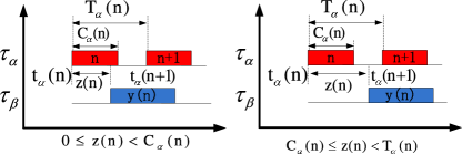
Figure 1: Case 1. The $y(n)$-th instance of $\tau_{\beta}$ is requested within $[t_{\alpha}(n),t_{\alpha}(n+1)]$

.

In Fig. 1, we can see that if $0\leq z(n)<C_{\alpha}(n)$, then the execution of the $y(n)$-th instance of $\tau_{\beta}$ will start from $t_{\alpha}(n)+C_{\alpha}(n)$ since the execution of the $n$-th instance of $\tau_{\alpha}$ will postpone the $y(n)$-th instance of $\tau_{\beta}$. If $C_{\alpha}(n)\leq z(n)<T_{\alpha}(n)$, then the execution of the $y(n)$-th instance of $\tau_{\beta}$ will start from $t_{\alpha}(n)+z(n)$. Thus, the execution of the $y(n)$-th instance of $\tau_{\beta}$ will start from

$${\rm max}\{t_{\alpha}(n)+C_{\alpha}(n),t_{\alpha}(n)+z(n)\}.$$

The time allocated for the execution of the $y(n)$-th instance of $\tau_{\beta}$ within $[t_{\alpha}(n),t_{\alpha}(n+1)]$ is,

$$t_{\alpha}(n+1)-{\rm max}\{t_{\alpha}(n)+C_{\alpha}(n),t_{\alpha}(n)+z(n)\}$$ (14)

$$= T_{\alpha}(n)-{\rm max}\{C_{\alpha}(n),z(n)\}$$ (15)

Therefore, the residue for the $y(n)$-th instance of $\tau_{\beta}$ to be computed after $t_{\alpha}(n+1)$ is

$$C_{\beta}(y(n))-(T_{\alpha}(n)-{\rm max}\{C_{\alpha}(n),z(n)\}).$$ (16)

The value of $P(n+1)$ can not be negative. Therefore

$$P(n+1)={\rm max}\{0,C_{\beta}(y(n))-(T_{\alpha}(n)-{\rm max}\{C_{\alpha}(n),z(n)\})\}.$$ (17)

Case 2: When the phase variable $z(n)$ satisfies

$$z(n)\geq T_{\alpha}(n)$$ (18)

which implies that the $y(n)$-th instance of $\tau_{\beta}$ is requested after $t_{\alpha}(n+1)$, the $\{y(n)-1\}$-th instance of $\tau_{\beta}$ is requested before $t_{\alpha}(n)$, and no instance of $\tau_{\beta}$ is requested within $[t_{\alpha}(n),t_{\alpha}(n+1)]$, as illustrated by Fig. 2 .

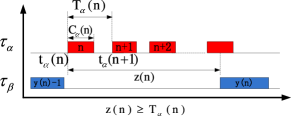
Figure 2: Case 2. The $y(n)$-th instance of $\tau_{\beta}$ is requested after $t_{\alpha}(n+1)$

In this case, the $\{y(n)-1\}$-th instance of $\tau_{\beta}$ is the last instance of $\tau_{\beta}$ requested before $t_{\alpha}(n)$. By definition, we know that $P(n)$ describes the remaining time to compute the $\{y(n)-1\}$-th instance of $\tau_{\beta}$ after $t_{\alpha}(n)$. In addition, the $\{y(n)-1\}$-th instance of $\tau_{\beta}$ is also the last instance of $\tau_{\beta}$ requested before $t_{\alpha}(n+1)$ and thus $P(n+1)$ describes the remaining time to compute the $\{y(n)-1\}$-th instance of $\tau_{\beta}$ after $t_{\alpha}(n+1)$.

From Fig. 2, we can see that the time that can be allocated to compute the $\{y(n)-1\}$-th instance of $\tau_{\beta}$ within $[t_{\alpha}(n),t_{\alpha}(n+1)]$ is $T_{\alpha}(n)-C_{\alpha}(n)$. Therefore, the remaining time for the $\{y(n)-1\}$-th instance of $\tau_{\beta}$ to be computed after $t_{\alpha}(n)$ is

$$P(n)-(T_{\alpha}(n)-C_{\alpha}(n)).$$

Thus the value of $P(n+1)$ is given by the following:

$$P(n+1)={\rm max}\{0,P(n)-(T_{\alpha}(n)-C_{\alpha}(n))\}.$$ (19)

According to (17) and (19), we can draw a conclusion on the transition rules for the state variable $P(n)$ from $n$ to $n+1$.

$$P(n+1)=\left\{\begin{array}[]{l}{\rm max}\{0,C_{\beta}(y(n))-(T_{\alpha}(n)\\ \;\;\;\;\;\;\;\;\;\;\;\;\;\;\;\;\;\;\;\;\;\;\;\;\;\;\;\;\;\;-{\rm max}\{C_{\alpha}(n),z(n)\})\}\\ \;\;\;\;\;\;\;\;\;\mbox{ if }\;\;0\leq z(n)<T_{\alpha}(n)\\ {\rm max}\{0,P(n)-(T_{\alpha}(n)-C_{\alpha}(n))\}\\ \;\;\;\;\;\;\;\;\;\mbox{ if }\;\;z(n)\geq T_{\alpha}(n)\end{array}\right.$$ (20)

IV-C Initialization of State Variables

In this subsection, we will discuss the initialization of the state variables within $[t_{0},t_{0}+L]$.

Suppose $t_{\alpha}$ and $t_{\beta}$ is the request time of the first instance of $\tau_{\alpha}$ and $\tau_{\beta}$ requested within $[t_{0},t_{0}+L]$ , $P_{\alpha}$ and $P_{\beta}$ is the residue for the last instance of $\tau_{\alpha}$ and $\tau_{\beta}$ requested before $t_{0}$ to be computed after $t_{0}$. $P_{\alpha}$ and $P_{\beta}$ need to be retrieved from the memory of the system.

We always assume that $t_{\alpha}(1)=t_{0}$. If $t_{0}\neq t_{\alpha}$, we will model a new instance of $\tau_{\alpha}$ as the first instance of $\tau_{\alpha}$ requested within $[t_{0},t_{0}+L]$. The new instance has the following task characteristics:

$$t_{\alpha}(1)=t_{0}\;\;\;C_{\alpha}(1)=P_{\alpha}\;\;\;T_{\alpha}(1)=t_{\alpha}(1)-t_{0}.$$ (21)

According to the definition of $t_{\beta}$, $P$, $y$ and $z$, we have

$$t_{\beta}(1)=t_{\beta}\;\;y(1)=1\;\;z(1)=t_{\beta}(1)-t_{\alpha}(1)\;\;P(1)=P_{\beta}$$

As we can see, the residue $P$ serves to connect the state of processor before $t_{0}$ with the state of processor within $[t_{0},t_{0}+L]$. Our model has the advantage over the classical scheduling analysis because instead of storing for all task behaviors made before $t_{0}$, we only need to record the residue of each task and to start the model. Therefore, we can analysis the scheduled behaviors of tasks starting from any time and within any finite time window as long as Assumptions III.1 and III.2 are satisfied.

V Processor Utilization Waveform of Two Tasks

Suppose $\tau_{\alpha}$ and $\tau_{\beta}$ are schedulable. With the states and transition rules for the scheduling algorithm determined, we compute a function $\Phi(t)$ that describes the states of the processor as either free ($\Phi(t)=0$) or busy ($\Phi(t)=1$). To achieve this goal, we study the states of processor within each request interval of $\tau_{\alpha}$, i.e. $[t_{\alpha}(n),t_{\alpha}(n+1)]$. The result is a function of time $\Phi_{n}$: $t\to\{0,1\}$ where for $t\in[t_{\alpha}(n),t_{\alpha}(n+1)]$, $\Phi_{n}(t)=0$ if the processor is free, and $\Phi_{n}(t)=1$ if the processor is busy. If $\Phi_{n}(t)$ is known for all $n$, we are able to describe $\Phi(t)$ within $[t_{0},t_{0}+L]$. Note that we ignore the scheduling transients that may exist for the processor, then the graph of such a function resembles a square wave. Although the space of possible square wave functions on a compact interval is infinite dimensional, we find that for the scheduling policy introduced in Section III, the waveforms only have two modes.

Case 1 This describes the mode when the phase variable $z(n)$ satisfies

$$0\leq z(n)<T_{\alpha}(n),$$ (22)

which implies that the $y(n)$-th instance of $\tau_{\beta}$ is requested within $[t_{\alpha}(n),t_{\alpha}(n)+T_{\alpha}(n)]$.

There are two subcases.

Case 1.1: If the phase variable $z(n)$ satisfies

$$0\leq z(n)<C_{\alpha}(n),$$ (23)

which implies that the $y(n)$-th instance of $\tau_{\beta}$ is requested while the processor is computing $\tau_{\alpha}$, i.e. $t_{\beta}(y(n))\in[t_{\alpha}(n),t_{\alpha}(n)+C_{\alpha}(n)]$, as illustrated by the left picture in Fig. 1.

It can be observed in Fig. 1 that

$$\Phi_{n}(t)=1\;\;\mbox{ if }\;\;t\in\left[t_{\alpha}(n),t_{\alpha}(n)+C_{\alpha}(n)\right].$$ (24)

The $\{y(n)-1\}$-th instance of $\tau_{\beta}$ must have been finished before $t_{\alpha}(n)$ as a result of schedulability requirements. Thus, $R(n)=0$. In order to derive a unified formula for $\Phi_{n}$ later, we notice that (24) can be rewritten as

$$\Phi_{n}(t)=1\;\;\mbox{ if }\;\;t\in\left[t_{\alpha}(n),t_{\alpha}(n)+C_{\alpha}(n)+R(n)\right].$$ (25)

The execution of the $y(n)$-th instance of $\tau_{\beta}$ will start from $t_{\alpha}(n)+C_{\alpha}(n)$. The finishing time of the $y(n)$-th instance of $\tau_{\beta}$ within $[t_{\alpha}(n),t_{\alpha}(n+1)]$ have two possibilities:

1. If

   $$C_{\beta}(y(n))<T_{\alpha}(n)-C_{\alpha}(n)$$ (26)

   which implies that the execution of $\tau_{\beta}$ will be finished before $t_{\alpha}(n+1)$, then

   $$\begin{array}[]{c}\Phi_{n}(t)=1\;\;\mbox{ if }\\ t\in\left[t_{\alpha}(n)+C_{\alpha}(n),t_{\alpha}(n)+C_{\alpha}(n)+C_{\beta}(y(n))\right].\end{array}$$ (27)

2. If

   $$C_{\beta}(y(n))\geq T_{\alpha}(n)-C_{\alpha}(n)$$ (28)

   which implies that the execution of $\tau_{\beta}$ will occupy the idle time of processor within the interval $[t_{\alpha}(n),t_{\alpha}(n+1)]$, then

   $$\begin{array}[]{c}\Phi_{n}(t)=1\;\;\mbox{ if }\\ t\in\left[t_{\alpha}(n)+C_{\alpha}(n),t_{\alpha}(n)+C_{\alpha}(n)+(T_{\alpha}(n)-C_{\alpha}(n))\right].\end{array}$$ (29)

As a summary, the execution time of the $y(n)$-th instance of $\tau_{\beta}$ during $[t_{\alpha}(n),t_{\alpha}(n+1)]$ is

$$\begin{array}[]{c}\Phi_{n}(t)=1\;\;\mbox{ if }\\ t\in\left[t_{\alpha}(n)+C_{\alpha}(n),t_{\alpha}(n)+C_{\alpha}(n)+\right.\\ \;\;\;\;\left.{\rm min}\{C_{\beta}(n),T_{\alpha}(n)-C_{\alpha}(n)\}\right].\end{array}$$ (30)

According to (25) and (30), the processor utilization during $[t_{\alpha}(n),t_{\alpha}(n+1)]$ is

$$\begin{array}[]{c}\Phi_{n}(t)=1\mbox{ if }\\ t\in\left[t_{\alpha}(n),t_{\alpha}(n)+C_{\alpha}(n)+R(n)\right]\bigcup\left[t_{\alpha}(n)+C_{\alpha}(n),\right.\\ \;\;\left.t_{\alpha}(n)+C_{\alpha}(n)+{\rm min}\{C_{\beta}(n),T_{\alpha}(n)-C_{\alpha}(n)\}\right].\end{array}$$ (31)

Case 1.2: If the phase variable $z(n)$ satisfies

$$z(n)\geq T_{\alpha}(n)$$ (32)

which implies that the $y(n)$-th instance of $\tau_{\beta}$ is requested within $[t_{\alpha}(n)+C_{\alpha}(n),t_{\alpha}(n+1)]$ , as shown in the right picture of Fig. 2.

The arguments for the $\{y(n)-1\}$th instance of $\tau_{\beta}$ still holds. Hence

$$\Phi_{n}(t)=1\;\;\mbox{ if }\;\;t\in\left[t_{\alpha}(n),t_{\alpha}(n)+C_{\alpha}(n)+R(n)\right].$$ (33)

The execution of the $y(n)$-th instance of $\tau_{\beta}$ will start from $t_{\alpha}(n)+z(n)$. The finishing time of the $y(n)$-th instance of $\tau_{\beta}$ within $[t_{\alpha}(n),t_{\alpha}(n+1)]$ have two possibilities. Using the similar method for (30), we can show that the execution time of the $y(n)$-th instance of $\tau_{\beta}$ during $[t_{\alpha}(n),t_{\alpha}(n+1)]$ is

$$\begin{array}[]{c}\Phi_{n}(t)=1\;\;\;\mbox{ if }\\ t\in\left[t_{\alpha}(n)+z(n),t_{\alpha}(n)+z(n)+\right.\\ \left.\;\;\;\;\;{\rm min}\{C_{\beta}(y(n)),T_{\alpha}(n)-z(n)\}\right].\end{array}$$ (34)

According to (33) and (34), we know that the processor utilization during $[t_{\alpha}(n),t_{\alpha}(n+1)]$ is

$$\begin{array}[]{c}\Phi_{n}(t)=1\;\;\mbox{ if }\\ t\in\left[t_{\alpha}(n),t_{\alpha}(n)+C_{\alpha}(n)+R(n)\right]\bigcup\left[t_{\alpha}(n)+z(n),\right.\\ \left.t_{\alpha}(n)+z(n)+{\rm min}\{C_{\beta}(y(n)),T_{\alpha}(n)-z(n)\}\right].\end{array}$$ (35)

As a summary, a conclusion can be drawn from (31) and (35) that during $[t_{\alpha}(n),t_{\alpha}(n+1)]$, the processor state is

$$\begin{array}[]{c}\Phi_{n}(t)=1\;\;\mbox{ if }\\ t\in\left[t_{\alpha}(n),t_{\alpha}(n)+C_{\alpha}(n)+R(n)\right]\bigcup\left[t_{\alpha}(n)+\right.\\ \left.{\rm max}\{C_{\alpha}(n),z(n)\},t_{\alpha}(n)+{\rm max}\{C_{\alpha}(n),z(n)\}\right.\\ \left.+{\rm min}\{C_{\beta}(y(n)),T_{\alpha}(n)-{\rm max}\{C_{\alpha}(n),z(n)\}\}\right].\end{array}$$ (36)

Case 2 This describes the mode when the phase variable $z(n)$ satisfies

$$z(n)\geq T_{\alpha}(n).$$ (37)

which implies that the $y(n)$-th instance of $\tau_{\beta}$ is requested after $t_{\alpha}(n+1)$, as shown in Fig. 2.

In Fig. 2, only the $\{y(n)-1\}$-th instance of $\tau_{\beta}$ and the $n$-th instance of $\tau_{\alpha}$ will affect the processor state within $[t_{\alpha}(n),t_{\alpha}(n+1)]$. In this case, the $\{y(n)-1\}$-th instance of $\tau_{\beta}$ is the last instance of $\tau_{\beta}$ requested before $t_{\alpha}(n)$. Thus, the execution of the $\{y(n)-1\}$-th instance of $\tau_{\beta}$ and the $n$-th instance of $\tau_{\alpha}$ will take up the time

$$R(n)+C_{\alpha}(n)$$

which implies that the processor state during $[t_{\alpha}(n),t_{\alpha}(n+1)]$ is

$$\Phi_{n}(t)=1\;\;\mbox{ if }\;\;t\in\left[t_{\alpha}(n),t_{\alpha}(n)+C_{\alpha}(n)+R(n)\right].$$ (38)

According to (36) and (38), the processor utilization within each request interval of $\tau_{\alpha}$ are depicted in Fig. 3.

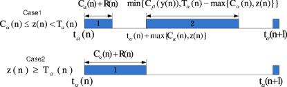
Figure 3: Processor Utilization Waveform within $[t_{\alpha}(n),t_{\alpha}(n+1)]$

VI Model For Multiple Tasks

In Section IV and V, we derive the processor utilization waveform of two tasks from a dynamic scheduling model. In this section, we develop a recursive algorithm to extend the modeling effort from two tasks to multiple tasks. Suppose $\tau_{1},...,\tau_{N}$ are schedulable. The processor utilization waveform of $\tau_{1},...,\tau_{N}$ can also be derived recursively in the following ways

1. Initialization: In the first recursion, we use $\tau_{\alpha}$ to denote $\tau_{1}$ and $\tau_{\beta}$ to denote $\tau_{2}$. Then, we derive the processor utilization waveform of $\tau_{\alpha}$ and $\tau_{\beta}$ according to (36) and (38), and model the waveform into a single task $\tau_{cmb}$.

2. Iteration: In the $n$-th iteration ($2\leq n\leq N-2$), we use $\tau_{\alpha}$ to denote the $\tau_{cmb}$ derived from the $(n-1)$-th iteration and $\tau_{\beta}$ to denote $\tau_{n+1}$. Then, we model the processor utilization waveform of $\tau_{\alpha}$ and $\tau_{\beta}$ into a single task $\tau_{cmb}$.

3. Result: In the $\{N-1\}$-th iteration, the processor utilization waveform of $\tau_{\alpha}$ and $\tau_{\beta}$ is actually the processor utilization waveform of $\tau_{1},...,\tau_{N}$

As we can see, the scheduling of multiple tasks are treated recursively as the scheduling of two tasks. There are two challenges in the recursive algorithm. First, we need to model the processor utilization waveform as a single task $\tau_{cmb}$; second, we need to prove that the Assumption III.1 and III.2 are satisfied during each iteration.

First, we show how to characterize $\tau_{cmb}$ as a single schedulable task from the processor utilization waveform. The processor utilization waveform within $[t_{\alpha}(n),t_{\alpha}(n+1)]$ have two modes. If $0\leq z(n)<T_{\alpha}(n)$, as illustrated in the upper figure of Fig. 3, the waveform within $[t_{\alpha}(n),t_{\alpha}(n+1)]$ is divided into two segments. Each segment can be viewed as the execution of one instance of $\tau_{cmb}$. The task behaviors of the first instance is

$$\left\{\begin{array}[]{l}{\rm Request\;Interval}:{\rm max}\{C_{\alpha}(n),z(n)\}\\ {\rm Computing\;Time}:C_{\alpha}(n)+R(n)\end{array}\right.$$ (39)

and the task behaviors of the second instance is

$$\left\{\begin{array}[]{l}{{\rm Request\;Interval}}:T_{\alpha}(n)-{\rm max}\{C_{\alpha}(n),z(n)\}\\ {\rm Computing\;Time}:\\ \;\;\;\;{\rm min}\{C_{\beta}(y(n)),T_{\alpha}(n)-{\rm max}\{C_{\alpha}(n),z(n)\}\}\end{array}\right.$$ (40)

On the other hand, if $z(n)\geq T_{\alpha}(n)$, as illustrated in the lower figure of Fig. 3, the waveforms within $[t_{\alpha}(n),t_{\alpha}(n+1)]$ can be viewed as the execution of one instance of $\tau_{cmb}$, with the task behavior being

$$\left\{\begin{array}[]{l}{\rm Request\;Interval}:T_{\alpha}(n)\\ {\rm Computing\;Time}:C_{\alpha}(n)+R(n)\end{array}\right.$$ (41)

Next, we use mathematical induction method to prove the following Proposition.

Proposition VI.1

In each iteration, for any time instant $t$, there exists $t_{0}$ and $L$ such that the maximum request interval of $\tau_{\alpha}$ is smaller than the minimal request interval of $\tau_{\beta}$ within $[t_{0},t_{0}+L]$.

Proof:

In the first iteration, $\tau_{\alpha}$ denotes $\tau_{1}$ and $\tau_{\beta}$ denotes $\tau_{2}$. According to Assumption III.1 and Assumption III.2, the Proposition VI.1 holds.

Suppose in the $n$-th iteration, for any time instant $t$, there exists $t_{0}$ and $L$ such that the maximum request interval of $\tau_{\alpha}$ is smaller than the minimum request interval of $\tau_{\beta}$ within $[t_{0},t_{0}+L]$. $\tau_{\beta}$ denotes $\tau_{n+1}$. Since $\tau_{cmb}$ is derived from each request interval of $\tau_{\alpha}$, the maximum request interval of $\tau_{cmb}$ is no larger than the maximum request interval of $\tau_{\alpha}$. According to Assumption III.1, we know that the maximum request interval of $\tau_{n+1}$ is smaller than the minimum request interval of $\tau_{n+2}$ within $[t_{0},t_{0}+L]$. Therefore, the maximum request interval of $\tau_{cmb}$ is smaller than the minimum request interval of $\tau_{n+2}$ within $[t_{0},t_{0}+L]$ and Proposition VI.1 in the $\{n+1\}$-th iteration holds. ∎

VII Simulations

In this section, we verify the dynamic scheduling model by comparing task scheduling waveforms with those generated by TrueTime. Then, we simulate the scheduling and the battery models together to predict remaining battery capacity.

VII-A Scheduling model verification

Consider the following scenario:

1. Initially, two periodic tasks $\tau_{1}$ and $\tau_{2}$ are running on a single processor, with the following parameters: $C_{1}=0.2{\rm min}$, $T_{1}=1{\rm min}$ $C_{2}=0.3{\rm min}$, $T_{1}=1.5{\rm min}$. $\tau_{1}$ starts at the time $0$ while $\tau_{2}$ starts at the time $0.3{\rm min}$;

2. An aperiodic task $\tau_{3}$ arrives at $50{\rm min}$ and another aperiodic task $\tau_{4}$ arrives at $50.6{\rm min}$. Both $\tau_{3}$ and $\tau_{4}$ will stop after $57.1{\rm min}$. Within $[50.6,57.1]$, $\tau_{3}$ and $\tau_{4}$ have the following characteristics $T_{3}(1)=1.6{\rm min}$, $C_{3}(1)=0.5{\rm min}$, $T_{3}(2)=2{\rm min}$, $C_{3}(2)=0.6{\rm min}$, $T_{3}(3)=1.7{\rm min}$, $C_{3}(3)=0.2{\rm min}$, $T_{3}(4)=1.8{\rm min}$, $C_{3}(4)=0.4{\rm min}$, $T_{4}(1)=2.5{\rm min}$, $C_{4}(1)=0.1{\rm min}$, $T_{4}(2)=3{\rm min}$, $C_{4}(2)=0.4{\rm min}$, $T_{4}(3)=1{\rm min}$, $C_{4}(3)=0.3{\rm min}$.

3. At time $110{\rm min}$, $\tau_{2}$ stops. Another periodic task $\tau_{5}$ arrives at $111.3{\rm min}$, with $T_{5}=1.2{\rm min}$ and $C_{5}=0.4{\rm min}$.

4. A aperiodic task $\tau_{6}$ arrives at time $113{\rm min}$ and disappears after $120{\rm min}$. Within $[113,120]$, $\tau_{6}$ has the following characteristics $T_{6}(1)=4{\rm min}$, $T_{6}(2)=3{\rm min}$, $C_{6}(1)=0.6{\rm min}$, $C_{6}(2)=0.3{\rm min}$.

We are interested in the state of processor within $[50,57.1]$ and $[110,120]$. The waveforms shown in Fig.4 and Fig.5 are consistent with those generated by Truetime. However, by using truetime, we have to initialize system whenever new tasks arrive and to simulate from the beginning.

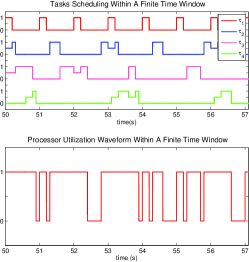
Figure 4: The State of Processor within $[50,57.1]$

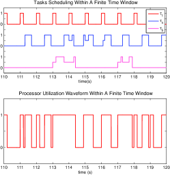
Figure 5: The State of Processor within $[110,120]$

As we can see in Fig.4 and 5, the value of a task will jump from $0$ to $1$ when it begins to execute. Then, the value of this task might go through several transitions between $1$ and $0.5$ during the execution period. Finally, the value of this task will fall back to $0$ once the execution is finished.

VII-B SPSB simulation

Fig. 6 shows the variation of battery capacity depending on processor status. When processor is busy, i.e. $\Phi(t)=1$, the battery capacity loss keeps increasing. When processor is free, i.e. $\Phi(t)=0$, the battery capacity loss begins to decrease due to the recovery effect.

We simulate a battery same as that in [22], which has the parameters $\alpha=40375$ and $\beta=0.273$. We assume that the current drawn by the processor when it is busy is $I=200$ mA and the current vanishes when the processor is free.

Fig. 6 shows the state of battery within two time windows $[50,57.1]$ and $[110,120]$. According to Assumption III.1 and III.2, we know that the state of the battery within its whole life period can be monitored by properly shifting the finite time window.

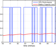
Figure 6: Simulating the hybrid model within [50 57.1]

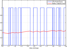
Figure 7: Simulating the hybrid model within [110 120]

VIII Conclusions

In this paper, we have established analytical models for the behaviors of multiple aperiodic tasks scheduled on a single processor supported by a single battery. We assume that the tasks are scheduled under a RMS like algorithm that assigns priority of tasks based on information within a finite time window. Our model is presented using a set of nonlinear difference equations that describe the task behaviors together with continuous differential equations that describe battery discharge behavior. One may find that these equations can be studied as a hybrid system. It can be perceived that through our modeling effort, battery behavior and scheduled task behaviors can now be studied jointly within the same theoretical framework. This fact is well aligned with the goals of cyber physical systems theory.

References

- [1] T. Chantem, X. S. Hu, and M. Lemmon, “Generalized elastic scheduling,” in Proc. of 27th IEEE Real-Time Systems Symposium (RTSS), 2006, pp. 236-245.
- [2] F. Xia and Y. Sun, “Control-scheduling codesign: A perspective on integrating control and computing,” in Dynamics of Continuous, Discrete and Impulsive Systems - Series B: Applications and Algorithms, Special Issue on ICSCA’06. Rome, Italy: Watam Press, 2006, pp. 1352–1358.
- [3] D. Seto, J. P. Lehoczky, L. Sha, and K. G. Shin, “Trade-off analysis of real-time control performance and schedulability,” Real-Time Systems, vol. 21, no. 3, pp. 199–217, 2001.
- [4] Q. He, H. Gan, and D. Jiao, “Explicit time-domain finite-element method stabilized for an arbitrarily large time step,” IEEE Trans. Antennas Propagation, vol. 60, no. 11, pp. 5240- 5250, Nov. 2012
- [5] N. Kottenstette, X. Koutsoukos, J. Hall, J. Sztipanovits, and P. Antsaklis, “Passivity-based design of wireless networked control systems for robustness to time-varying delays,” in Proc. IEEE 29th Real-Time Systems Symposium (RTSS), 2008, pp. 15–24.
- [6] F. Zhang, and Z. Shi, “Optimal and Adaptive Battery Discharge Strategies for Cyber-Physical Systems,” in Proc. of 48th IEEE Conference on decision and control, 2009, pp 6232-6237.
- [7] C.-F. Chiasserini and R. Rao, “Energy efficient battery management,” IEEE Journal on Selected Areas in Communications, vol. 19, no. 7, pp. 1235–1245, 2001.
- [8] R. Rao, S. Vrudhula, and D. N. Rakhmatov, “Battery modeling for energy-aware system design,” Computer, vol. 36, no. 12, pp. 77–87, 2003.
- [9] Q. He, D. Chen, and D. Jiao, “From layout directly to simulation: A first-principle-guided circuit simulator of linear complexity and its efficient parallelization,” IEEE Trans. Components, Packaging and Manufacturing Technology, vol. 2, no. 4, pp. 687 -699, Apr. 2012.
- [10] Q. He and D. Jiao, “Fast Electromagnetics-Based Co-Simulation of Linear Network and Nonlinear Circuits for the Analysis of High-Speed Integrated Circuits,” IEEE Trans. Microwave Theory and Techniques, vol. 58, no. 12, pp. 3677–3687, Nov. 2010
- [11] M. Doyle, T. Fuller, and J. Newman, “Modeling of galvanostatic charge and discharge of the lithium/polymer/insertion cell,” Journal of Electrochemical Society, vol. 140, no. 6, pp. 1526–1533, 1995.
- [12] D. Linden and T. Reddy, Handbook of Batteries, 3rd ed. McGraw-Hill, 2001.
- [13] M. Chen and G. A. Rincon-Mora, “Accurate electrical battery model capable of predicting runtime and performance,” IEEE transactions on energy conversion, vol. 21, pp. 504–511, 2006.
- [14] Q. He, D. Chen, and D. Jiao, “An Explicit and Unconditionally Stable Time-Domain Finite-Element Method of Linear Complexity for Electromagnetics-Based Simulation of 3-D Global Interconnect Network,” IEEE Conf. Electrical Performance of Electronic Packaging and and Systems (EPEPS), pp. 185 -188, Oct. 2011
- [15] J. M. Rabaey, Digital Integrated Circuts: A Design Perspective. Prentice-Hall, 1996.
- [16] F. Yao, A. Demers, and S. Shenker, “A scheduling model for reduced CPU energy,” in Proc. IEEE 36th Annual FOCS, 1995, pp. 374–382.
- [17] A. Rowe, K. Lakshmanan, Z. Haifeng, and R. Rajkumar, “Rate-harmonized scheduling for saving energy,” in Proc. IEEE 29th Real-Time Systems Symposium (RTSS), 2008, pp. 113–122.
- [18] Z. Ren, B. H. Krogh, and R. Marculescu, “Hierarchical adaptive dynamic power management,” IEEE Transactions on Computers, vol. 54, no. 4, pp. 409–420, 2005.
- [19] L. Jiong and N. K. Jha, “Power-efficient scheduling for heterogeneous distributed real-time embedded systems,” IEEE Transactions on Computer-Aided Design of Integrated Circuits and Systems, vol. 26, no. 6, pp. 1161–70, 2007.
- [20] L. Jiong, N. K. Jha, and P. Li-Shiuan, “Simultaneous dynamic voltage scaling of processors and communication links in real-time distributed embedded systems,” IEEE Transactions on VLSI Systems, vol. 15, no. 4, pp. 427–37, 2007.
- [21] F. Zhang, Z. Shi, and W. Wolf, “A dynamic battery model for co-design in cyber-physical systems,” in Proc. of 2nd International Workshop on Cyber-Physical Systems (WCPS 2009), Montereal, Canada, 2009.
- [22] D. Rakhmatov, S. Vrudhula, and D. A. Wallach, “A model for battery lifetime analysis for organizing applications on a pocket computer,” IEEE Transactions on VLSI Systems, vol. 11, no. 6, pp. 1019–1030, 2003.
- [23] A. Cervin, D. Henriksson, B. Lincoln, J. Eker, and K.-E. Arzen, “How does control timing affect performance,” IEEE Control Systems Magazine, no. 6, pp. 16–30, 2003.
- [24] C. L. Liu and J. W. Layland, “Scheduling algorithms for multiprogramming in a Hard-Real-Time environment,” Journal of the ACM, vol. 20, no. 1, pp. 46–61, 1973.
- [25] J. Lehoczky, L. Sha, and Y. Ding, “The rate monotonic scheduling algorithm: Exact characterization and average case behavior,” in Proc. IEEE 10th Real-Time Systems Symposium (RTSS), 1989, pp. 166–171.
- [26] E. Bini, G. C. Buttazzo, and G. M. Buttazzo, “Rate monotonic analysis: the hyperbolic bound,” IEEE Trans. on Computers, vol. 52, no. 7, pp. 933–42, 2003.
- [27] X. D. Koutsoukos, P. J. Antsaklis, J. A. Stiver, and M. D. Lemmon, “Supervisory control of hybrid systems,” Proceedings of the IEEE, vol. 88, no. 7, pp. 1026–49, 2000.
- [28] M. S. Branicky, “Multiple Lyapunov functions and other analysis tools for switched and hybrid systems,” IEEE Trans. Automat. Cont., vol. 43, pp. 475–482, 1998.