Approximating LZ77 via
Small-Space Multiple-Pattern Matching

Abstract

We generalize Karp-Rabin string matching to handle multiple patterns in $\mathcal{O}(n\log n+m)$ time and $\mathcal{O}(s)$ space, where $n$ is the length of the text and $m$ is the total length of the $s$ patterns, returning correct answers with high probability. As a prime application of our algorithm, we show how to approximate the LZ77 parse of a string of length $n$. If the optimal parse consists of $z$ phrases, using only $\mathcal{O}(z)$ working space we can return a parse consisting of at most $(1+\varepsilon)z$ phrases in $\mathcal{O}(\varepsilon^{-1}n\log n)$ time, for any $\varepsilon\in(0,1]$. As previous quasilinear-time algorithms for LZ77 use $\Omega(n/\text{poly}\log n)$ space, but $z$ can be exponentially small in $n$, these improvements in space are substantial.

1 Introduction

Multiple-pattern matching, the task of locating the occurrences of $s$ patterns of total length $m$ in a single text of length $n$, is a fundamental problem in the field of string algorithms. The algorithm by Aho and Corasick [2] solves this problem using $\mathcal{O}(n+m)$ time and $\mathcal{O}(m)$ working space in addition to the space needed for the text and patterns. To list all $\mathsf{occ}$ occurrences rather than, e.g., the leftmost ones, extra $\mathcal{O}(\mathsf{occ})$ time is necessary. When the space is limited, we can use a compressed Aho-Corasick automaton [11]. In extreme cases, one could apply a linear-time constant-space single-pattern matching algorithm sequentially for each pattern in turn, at the cost of increasing the running time to $\mathcal{O}(n\cdot s+m)$. Well-known examples of such algorithms include those by Galil and Seiferas [8], Crochemore and Perrin [5], and Karp and Rabin [13] (see [3] for a recent survey).

It is easy to generalize Karp-Rabin matching to handle multiple patterns in $\mathcal{O}(n+m)$ expected time and $\mathcal{O}(s)$ working space provided that all patterns are of the same length [10]. To do this, we store the fingerprints of the patterns in a hash table, and then slide a window over the text maintaining the fingerprint of the fragment currently in the window. The hash table lets us check if the fragment is an occurrence of a pattern. If so, we report it and update the hash table so that every pattern is returned at most once. This is a very simple and actually applied idea [1], but it is not clear how to extend it for patterns with many distinct lengths. In this paper we develop a dictionary matching algorithm which works for any set of patterns in $\mathcal{O}(n\log n+m)$ time and $\mathcal{O}(s)$ working space, assuming that read-only random access to the text and the patterns is available. If required, we can compute for every pattern its longest prefix occurring in the text, also in $\mathcal{O}(n\log n+m)$ time and $\mathcal{O}(s)$ working space.

In a very recent independent work Clifford et al. [4] gave a dictionary matching algorithm in the streaming model. In this setting the patterns and later the text are scanned once only (as opposed to read-only random access) and an occurrence needs to be reported immediately after its last character is read. Their algorithm uses $\mathcal{O}(s\log\ell)$ space and takes $\mathcal{O}(\log\log(s+\ell))$ time per character where $\ell$ is the length of the longest pattern ($\frac{m}{s}\leq\ell\leq m$). Even though some of the ideas used in both results are similar, one should note that the streaming and read-only models are quite different. In particular, computing the longest prefix occurring in the text for every pattern requires $\Omega(m\log\min(n,|\Sigma|))$ bits of space in the streaming model, as opposed to the $\mathcal{O}(s)$ working space achieved by our solution in the read-only setting.

As a prime application of our dictionary matching algorithm, we show how to approximate the Lempel-Ziv 77 (LZ77) parse [18] of a text of length $n$ using working space proportional to the number of phrases (again, we assume read-only random access to the text). Computing the LZ77 parse in small space is an issue of high importance, with space being a frequent bottleneck of today’s systems. Moreover, LZ77 is useful not only for data compression, but also as a way to speed up algorithms [15]. We present a general approximation algorithm working in $\mathcal{O}(z)$ space for inputs admitting LZ77 parsing with $z$ phrases. For any $\varepsilon\in(0,1]$, the algorithm can be used to produce a parse consisting of $(1+\varepsilon)z$ phrases in $\mathcal{O}(\varepsilon^{-1}n\log n)$ time.

To the best of our knowledge, approximating LZ77 factorization in small space has not been considered before, and our algorithm is significantly more efficient than methods producing the exact answer. A recent sublinear-space algorithm, due to Kärkkäinen et al. [12], runs in $\mathcal{O}(nd)$ time and uses $\mathcal{O}(n/d)$ space, for any parameter $d$. An earlier online solution by Gasieniec et al. [9] uses $\mathcal{O}(z)$ space and takes $\mathcal{O}(z^{2}\log^{2}z)$ time for each character appended. Other previous methods use significantly more space when the parse is small relative to $n$; see [7] for a recent discussion.

Structure of the paper.

Sect. 2 introduces terminology and recalls several known concepts. This is followed by the description of our dictionary matching algorithm. In Sect. 3 we show how to process patterns of length at most $s$ and in Sect. 4 we handle longer patterns, with different procedures for repetitive and non-repetitive ones. In Sect. 5 we extend the algorithm to compute, for every pattern, the longest prefix occurring in the text. Finally, in Sect. 7, we apply the dictionary matching algorithm to construct an approximation of the LZ77 parsing, and in Sect. 6 we explain how to modify the algorithms to make them Las Vegas.

Model of computation.

Our algorithms are designed for the word-RAM with $\Omega(\log n)$-bit words and assume integer alphabet of polynomial size. The usage of Karp-Rabin fingerprints makes them Monte Carlo randomized: the correct answer is returned with high probability, i.e., the error probability is inverse polynomial with respect to input size, where the degree of the polynomial can be set arbitrarily large. With some additional effort, our algorithms can be turned into Las Vegas randomized, where the answer is always correct and the time bounds hold with high probability. Throughout the whole paper, we assume read-only random access to the text and the patterns, and we do not include their sizes while measuring space consumption.

2 Preliminaries

We consider finite words over an integer alphabet $\Sigma=\{0,\ldots,\sigma-1\}$, where $\sigma=\text{poly}(n+m)$. For a word $w=w[1]\ldots w[n]\in\Sigma^{n}$, we define the length of $w$ as $|w|=n$. For $1\leq i\leq j\leq n$, a word $u=w[i]\ldots w[j]$ is called a subword of $w$. By $w[i..j]$ we denote the occurrence of $u$ at position $i$, called a fragment of $w$. A fragment with $i=1$ is called a prefix and a fragment with $j=n$ is called a suffix.

A positive integer $p$ is called a period of $w$ whenever $w[i]=w[i+p]$ for all $i=1,2,\ldots,|w|-p$. In this case, the prefix $w[1..p]$ is often also called a period of $w$. The length of the shortest period of a word $w$ is denoted as $\operatorname{per}(w)$. A word $w$ is called periodic if $\operatorname{per}(w)\leq\frac{|w|}{2}$ and highly periodic if $\operatorname{per}(w)\leq\frac{|w|}{3}$. The well-known periodicity lemma [6] says that if $p$ and $q$ are both periods of $w$, and $p+q\leq|w|$, then $\gcd(p,q)$ is also a period of $w$. We say that word $w$ is primitive if $\operatorname{per}(w)$ is not a proper divisor of $|w|$. Note that the shortest period $w[1..\operatorname{per}(w)]$ is always primitive.

2.1 Fingerprints

Our randomized construction is based on Karp-Rabin fingerprints; see [13]. Fix a word $w[1..n]$ over an alphabet $\Sigma=\{0,\ldots,\sigma-1\}$, a constant $c\geq 1$, a prime number $p>\max(\sigma,n^{c+4})$, and choose $x\in\mathbb{Z}_{p}$ uniformly at random. We define the fingerprint of a subword $w[i..j]$ as $\Phi(w[i..j])=w[i]+w[i+1]x+\ldots+w[j]x^{j-i}\bmod{p}$. With probability at least $1-\frac{1}{n^{c}}$, no two distinct subwords of the same length have equal fingerprints. The situation when this happens for some two subwords is called a false-positive. From now on when stating the results we assume that there are no false-positives to avoid repeating that the answers are correct with high probability. For dictionary matching, we assume that no two distinct subwords of $w=TP_{1}\ldots P_{s}$ have equal fingerprints. Fingerprints let us easily locate many patterns of the same length. A straightforward solution described in the introduction builds a hash table mapping fingerprints to patterns. However, then we can only guarantee that the hash table is constructed correctly with probability $1-\mathcal{O}(\frac{1}{s^{c}})$ (for an arbitrary constant $c$), and we would like to bound the error probability by $\mathcal{O}(\frac{1}{(n+m)^{c}})$. Hence we replace hash table with a deterministic dictionary as explained below. Although it increases the time by $\mathcal{O}(s\log s)$, the extra term becomes absorbed in the final complexities.

Theorem 1.

Given a text $T$ of length $n$ and patterns $P_{1},\ldots,P_{s}$, each of length exactly $\ell$, we can compute the the leftmost occurrence of every pattern $P_{i}$ in $T$ using $\mathcal{O}(n+s\ell+s\log s)$ total time and $\mathcal{O}(s)$ space.

Proof.

We calculate the fingerprint $\Phi(P_{j})$ of every pattern. Then we build in $\mathcal{O}(s\log s)$ time [16] a deterministic dictionary $\mathcal{D}$ with an entry mapping $\Phi(P_{j})$ to $j$. For multiple identical patterns we create just one entry, and at the end we copy the answers to all instances of the pattern. Then we scan the text $T$ with a sliding window of length $\ell$ while maintaining the fingerprint $\Phi(T[i..i+\ell-1])$ of the current window. Using $\mathcal{D}$, we can find in $\mathcal{O}(1)$ time an index $j$ such that $\Phi(T[i..i+\ell-1])=\Phi(P_{j})$, if any, and update the answer for $P_{j}$ if needed (i.e., if there was no occurrence of $P_{j}$ before). If we precompute $x^{-1}$, the fingerprints $\Phi(T[i..i+\ell-1])$ can be updated in $\mathcal{O}(1)$ time while increasing $i$.

∎

2.2 Tries

A trie of a collection of strings $P_{1},\ldots,P_{s}$ is a rooted tree whose nodes correspond to prefixes of the strings. The root represents the empty word and the edges are labeled with single characters. The node corresponding to a particular prefix is called its locus. In a compacted trie unary nodes that do not represent any $P_{i}$ are dissolved and the labels of their incidents edges are concatenated. The dissolved nodes are called implicit as opposed to the explicit nodes, which remain stored. The locus of a string in a compacted trie might therefore be explicit or implicit. All edges outgoing from the same node are stored on a list sorted according to the first character, which is unique among these edges. The labels of edges of a compacted trie are stored as pointers to the respective fragments of strings $P_{i}$. Consequently, a compacted trie can be stored in space proportional to the number of explicit nodes, which is $\mathcal{O}(s)$.

Consider two compacted tries $\mathcal{T}_{1}$ and $\mathcal{T}_{2}$. We say that (possibly implicit) nodes $v_{1}\in\mathcal{T}_{1}$ and $v_{2}\in\mathcal{T}_{2}$ are twins if they are loci of the same string. Note that every $v_{1}\in\mathcal{T}_{1}$ has at most one twin $v_{2}\in\mathcal{T}_{2}$.

Lemma 2.

Given two compacted tries $\mathcal{T}_{1}$ and $\mathcal{T}_{2}$ constructed for $s_{1}$ and $s_{2}$ strings, respectively, in $\mathcal{O}(s_{1}+s_{2})$ total time and space we can find for each explicit node $v_{1}\in\mathcal{T}_{1}$ a node $v_{2}\in\mathcal{T}_{2}$ such that if $v_{1}$ has a twin in $\mathcal{T}_{2}$, then $v_{2}$ is its twin. (If $v_{1}$ has no twin in $\mathcal{T}_{2}$, the algorithm returns an arbitrary node $v_{2}\in\mathcal{T}_{2}$).

Proof.

We recursively traverse both tries while maintaining a pair of nodes $v_{1}\in\mathcal{T}_{1}$ and $v_{2}\in\mathcal{T}_{2}$, starting with the root of $\mathcal{T}_{1}$ and $\mathcal{T}_{2}$ satisfying the following invariant: either $v_{1}$ and $v_{2}$ are twins, or $v_{1}$ has no twin in $\mathcal{T}_{2}$. If $v_{1}$ is explicit, we store $v_{2}$ as the candidate for its twin. Next, we list the (possibly implicit) children of $v_{1}$ and $v_{2}$ and match them according to the edge labels with a linear scan. We recurse on all pairs of matched children. If both $v_{1}$ and $v_{2}$ are implicit, we simply advance to their immediate children. The last step is repeated until we reach an explicit node in at least one of the tries, so we keep it implicit in the implementation to make sure that the total number of operations is $\mathcal{O}(s_{1}+s_{2})$. If a node $v\in\mathcal{T}_{1}$ is not visited during the traversal, for sure it has no twin in $\mathcal{T}_{2}$. Otherwise, we compute a single candidate for its twin. ∎

3 Short Patterns

To handle the patterns of length not exceeding a given threshold $\ell$, we first build a compacted trie for those patterns. Construction is easy if the patterns are sorted lexicographically: we insert them one by one into the compacted trie first naively traversing the trie from the root, then potentially partitioning one edge into two parts, and finally adding a leaf if necessary. Thus, the following result suffices to efficiently build the tries.

Lemma 3.

One can lexicographically sort strings $P_{1},\ldots,P_{s}$ of total length $m$ in $\mathcal{O}(m+\sigma^{\varepsilon})$ time using $\mathcal{O}(s)$ space, for any constant $\varepsilon>0$.

Proof.

We separately sort the $\sqrt{m}+\sigma^{\varepsilon/2}$ longest strings and all the remaining strings, and then merge both sorted lists. Note these longest strings can be found in $\mathcal{O}(s)$ time using a linear time selection algorithm.

Long strings are sorted using insertion sort. If the longest common prefixes between adjacent (in the sorted order) strings are computed and stored, inserting $P_{j}$ can be done in $\mathcal{O}(j+|P_{j}|)$ time. In more detail, let $S_{1},S_{2},\ldots,S_{j-1}$ be the sorted list of already processed strings. We start with $k:=1$ and keep increasing $k$ by one as long as $S_{k}$ is lexicographically smaller than $P_{j}$ while maintaining the longest common prefix between $S_{k}$ and $P_{j}$, denoted $\ell$. After increasing $k$ by one, we update $\ell$ using the longest common prefix between $S_{k-1}$ and $S_{k}$, denoted $\ell^{\prime}$, as follows. If $\ell^{\prime}>\ell$, we keep $\ell$ unchanged. If $\ell^{\prime}=\ell$, we try to iteratively increase $\ell$ by one as long as possible. In both cases, the new value of $\ell$ allows us to lexicographically compare $S_{k}$ and $P_{j}$ in constant time. Finally, $\ell^{\prime}<\ell$ guarantees that $P_{j}<S_{k}$ and we may terminate the procedure. Sorting the $\sqrt{m}+\sigma^{\varepsilon/2}$ longest strings using this approach takes $\mathcal{O}(m+(\sqrt{m}+\sigma^{\varepsilon/2})^{2})=\mathcal{O}(m+\sigma^{\varepsilon})$ time.

The remaining strings are of length at most $\sqrt{m}$ each, and if there are any, then $s\geq\sigma^{\varepsilon/2}$. We sort these strings by iteratively applying radix sort, treating each symbol from $\Sigma$ as a sequence of $\frac{2}{\varepsilon}$ symbols from $\{0,1,\ldots,\sigma^{\varepsilon/2}-1\}$. Then a single radix sort takes time and space proportional to the number of strings involved plus the alphabet size, which is $\mathcal{O}(s+\sigma^{\varepsilon/2})=\mathcal{O}(s)$. Furthermore, because the numbers of strings involved in the subsequent radix sorts sum up to $m$, the total time complexity is $\mathcal{O}(m+\sigma^{\varepsilon/2}\sqrt{m})=\mathcal{O}(m+\sigma^{\varepsilon})$.

Finally, the merging takes time linear in the sum of the lengths of all the involved strings, so the total complexity is as claimed. ∎

Next, we partition $T$ into $\mathcal{O}(\frac{n}{\ell})$ overlapping blocks $T_{1}=T[1..2\ell]$, $T_{2}=T[\ell+1..3\ell]$, $T_{3}=T[2\ell+1..4\ell],\ldots$. Notice that each subword of length at most $\ell$ is completely contained in some block. Thus, we can consider every block separately.

The suffix tree of each block $T_{i}$ takes $\mathcal{O}(\ell\log\ell)$ time [17] and $\mathcal{O}(\ell)$ space to construct and store (the suffix tree is discarded after processing the block). We apply Lemma 2 to the suffix tree and the compacted trie of patterns; this takes $\mathcal{O}(\ell+s)$ time. For each pattern $P_{j}$ we obtain a node such that the corresponding subword is equal to $P_{j}$ provided that $P_{j}$ occurs in $T_{i}$. We compute the leftmost occurrence $T_{i}[b..e]$ of the subword, which takes constant time if we store additional data at every explicit node of the suffix tree, and then we check whether $T_{i}[b..e]=P_{j}$ using fingerprints. For this, we precompute the fingerprints of all patterns, and for each block $T_{i}$ we precompute the fingerprints of its prefixes in $\mathcal{O}(\ell)$ time and space, which allows to determine the fingerprint of any of its subwords in constant time.

In total, we spend $\mathcal{O}(m+\sigma^{\varepsilon})$ for preprocessing and $\mathcal{O}(\ell\log\ell+s)$ for each block. Since $\sigma=(n+m)^{\mathcal{O}(1)}$, for small enough $\varepsilon$ this yields the following result.

Theorem 4.

Given a text $T$ of length $n$ and patterns $P_{1},\ldots,P_{s}$ of total length $m$, using $\mathcal{O}(n\log\ell+s\frac{n}{\ell}+m)$ total time and $\mathcal{O}(s+\ell)$ space we can compute the leftmost occurrences in $T$ of every pattern $P_{j}$ of length at most $\ell$.

4 Long Patterns

To handle patterns longer than a certain threshold, we first distribute them into groups according to the value of $\lfloor\log_{4/3}|P_{j}|\rfloor$. Patterns longer than the text can be ignored, so there are $\mathcal{O}(\log n)$ groups. Each group is handled separately, and from now on we consider only patterns $P_{j}$ satisfying $\lfloor\log_{4/3}|P_{j}|\rfloor=i$.

We classify the patterns into classes depending on the periodicity of their prefixes and suffixes. We set $\ell=\lceil(4/3)^{i}\rceil$ and define $\alpha_{j}$ and $\beta_{j}$ as, respectively, the prefix and the suffix of length $\ell$ of $P_{j}$. Since $\frac{2}{3}(|\alpha_{j}|+|\beta_{j}|)=\frac{4}{3}\ell\geq|P_{j}|$, the following fact yields a classification of the patterns into three classes: either $P_{j}$ is highly periodic, or $\alpha_{j}$ is not highly periodic, or $\beta_{j}$ is not highly periodic. The intuition behind this classification is that if the prefix or the suffix is not repetitive, then we will not see it many times in a short subword of the text. On the other hand, if both the prefix and suffix are repetitive, then there is some structure that we can take advantage of.

Fact 5.

Suppose $x$ and $y$ are a prefix and a suffix of a word $w$, respectively. If $|x|+|y|\geq|w|+p$ and $p$ is a period of both $x$ and $y$, then $p$ is a period of $w$.

Proof.

We need to prove that $w[i]=w[i+p]$ for all $i=1,2,\ldots,|w|-p$. If $i+p\leq|x|$ this follows from $p$ being a period of $x$, and if $i\geq|w|-|y|+1$ from $p$ being a period of $y$. Because $|x|+|y|\geq|w|+p$, these two cases cover all possible values of $i$. ∎

To assign every pattern to the appropriate class, we compute the periods of $P_{j}$, $\alpha_{j}$ and $\beta_{j}$ using small space. Roughly the same result has been proved in [14], but for completeness we provide the full proof here.

Lemma 6.

Given a read-only string $w$ one can decide in $\mathcal{O}(|w|)$ time and constant space if $w$ is periodic and if so, compute $\operatorname{per}(w)$.

Proof.

Let $v$ be the prefix of $w$ of length $\lceil\frac{1}{2}|w|\rceil$ and $p$ be the starting position of the second occurrence of $v$ in $w$, if any. We claim that if $\operatorname{per}(w)\leq\frac{1}{2}|w|$, then $\operatorname{per}(w)=p-1$. Observe first that in this case $v$ occurs at a position $\operatorname{per}(w)+1$. Hence, $\operatorname{per}(w)\geq p-1$. Moreover $p-1$ is a period of $w[1..|v|+p-1]$ along with $\operatorname{per}(w)$. By the periodicity lemma, $\operatorname{per}(w)\leq\frac{1}{2}|w|\leq|v|$ implies that $\gcd(p-1,\operatorname{per}(w))$ is also a period of that prefix. Thus $\operatorname{per}(w)>p-1$ would contradict the primitivity of $w[1..\operatorname{per}(w)]$.

The algorithm computes the position $p$ using a linear time constant-space pattern matching algorithm. If it exists, it uses letter-by-letter comparison to determine whether $w[1..p-1]$ is a period of $w$. If so, by the discussion above $\operatorname{per}(w)=p-1$ and the algorithm returns this value. Otherwise, $2\operatorname{per}(w)>|w|$, i.e., $w$ is not periodic. The algorithm runs in linear time and uses constant space.

∎

4.1 Patterns without Long Highly Periodic Prefix

Below we show how to deal with patterns with non-highly periodic prefixes $\alpha_{j}$. Patterns with non-highly periodic suffixes $\beta_{j}$ can be processed using the same method after reversing the text and the patterns.

Lemma 7.

Let $\ell$ be an arbitrary integer. Suppose we are given a text $T$ of length $n$ and patterns $P_{1},\ldots,P_{s}$ such that for $1\leq j\leq s$ we have $\ell\leq|P_{j}|<\frac{4}{3}\ell$ and $\alpha_{j}=P_{j}[1..\ell]$ is not highly periodic. We can compute the leftmost and the rightmost occurrence of each pattern $P_{j}$ in $T$ using $\mathcal{O}(n+s(1+\frac{n}{\ell})\log s+s\ell)$ time and $\mathcal{O}(s)$ space.

The algorithm scans the text $T$ with a sliding window of length $\ell$. Whenever it encounters a subword equal to the prefix $\alpha_{j}$ of some $P_{j}$, it creates a request to verify whether the corresponding suffix $\beta_{j}$ of length $\ell$ occurs at the appropriate position. The request is processed when the sliding window reaches that position. This way the algorithm detects the occurrences of all the patterns. In particular, we may store the leftmost and rightmost occurrence of each pattern.

We use the fingerprints to compare the subwords of $T$ with $\alpha_{j}$ and $\beta_{j}$. To this end, we precompute $\Phi(\alpha_{j})$ and $\Phi(\beta_{j})$ for each $j$. We also build a deterministic dictionary $\mathcal{D}$ [16] with an entry mapping $\Phi(\alpha_{j})$ to $j$ for every pattern (if there are multiple patterns with the same value of $\Phi(\alpha_{j})$, the dictionary maps a fingerprint to a list of indices). These steps take $\mathcal{O}(s\ell)$ and $\mathcal{O}(s\log s)$, respectively. Pending requests are maintained in a priority queue $\mathcal{Q}$, implemented using a binary heap as pairs containing the pattern index (as a value) and the position where the occurrence of $\beta_{j}$ is anticipated (as a key).

1 for $i=1$ to $n-\ell+1$ do

2       $h:=\Phi(w[i..i+\ell-1])$

3       foreach $j:\Phi(\alpha_{j})=h$ do

4             add a request $(i+|P_{j}|-\ell,j)$ to $\mathcal{Q}$

5      foreach request $(i,j)\in\mathcal{Q}$ at position $i$ do

6             if $h=\Phi(\beta_{j})$ then

7                   report an occurrence of $P_{j}$ at $i+\ell-|P_{j}|$

8            remove $(i,j)$ from $\mathcal{Q}$

Algorithm 1 Processing patterns with non-highly periodic $\alpha_{j}$.

Algorithm 1 provides a detailed description of the processing phase. Let us analyze its time and space complexities. Due to the properties of Karp-Rabin fingerprints, line 1 can be implemented in $\mathcal{O}(1)$ time. Also, the loops in lines 1 and 1 takes extra $\mathcal{O}(1)$ time even if the respective collections are empty. Apart from these, every operation can be assigned to a request, each of them taking $\mathcal{O}(1)$ (lines 1 and 1-1) or $\mathcal{O}(\log|\mathcal{Q}|)$ (lines 1 and 1) time. To bound $|\mathcal{Q}|$, we need to look at the maximum number of pending requests.

Fact 8.

For any pattern $P_{j}$ just $\mathcal{O}(1+\frac{n}{\ell})$ requests are created and at any time at most one of them is pending.

Proof.

Note that there is a one-to-one correspondence between requests concerning $P_{j}$ and the occurrences of $\alpha_{j}$ in $T$. The distance between two such occurrences must be at least $\frac{1}{3}\ell$, because otherwise the period of $\alpha_{j}$ would be at most $\frac{1}{3}\ell$, thus making $\alpha_{j}$ highly periodic. This yields the $\mathcal{O}(1+\frac{n}{\ell})$ upper bound on the total number of requests. Additionally, any request is pending for at most $|P_{j}|-\ell<\frac{1}{3}\ell$ iterations of the main for loop. Thus, the request corresponding to an occurrence of $\alpha_{j}$ is already processed before the next occurrence appears. ∎

Hence, the scanning phase uses $\mathcal{O}(s)$ space and takes $\mathcal{O}(n+s(1+\frac{n}{\ell})\log s)$ time. Taking preprocessing into account, we obtain bounds claimed in Lemma 7.

4.2 Highly Periodic Patterns

Lemma 9.

Let $\ell$ be an arbitrary integer. Given a text $T$ of length $n$ and a collection of highly periodic patterns $P_{1},\ldots,P_{s}$ such that for $1\leq j\leq s$ we have $\ell\leq|P_{j}|<\frac{4}{3}\ell$, we can compute the leftmost occurrence of each pattern $P_{j}$ in $T$ using $\mathcal{O}(n+s(1+\frac{n}{\ell})\log s+s\ell)$ total time and $\mathcal{O}(s)$ space.

The solution is basically the same as in the proof of Lemma 7, except that the algorithm ignores certain shiftable occurrences. An occurrence of $x$ at position $i$ of $T$ is called shiftable if there is another occurrence of $x$ at position $i-\operatorname{per}(x)$. The remaining occurrences are called non-shiftable. Notice that the leftmost occurrence is always non-shiftable, so indeed we can safely ignore some of the shiftable occurrences of the patterns. Because $2\operatorname{per}(P_{j})\leq\frac{2}{3}|P_{j}|\leq\frac{8}{9}\ell<\ell$, the following fact implies that if an occurrence of $P_{j}$ is non-shiftable, then the occurrence of $\alpha_{j}$ at the same position is also non-shiftable.

Fact 10.

Let $y$ be a prefix of $x$ such that $|y|\geq 2\operatorname{per}(x)$. Suppose $x$ has a non-shiftable occurrence at position $i$ in $w$. Then, the occurrence of $y$ at position $i$ is also non-shiftable.

Proof.

Note that $\operatorname{per}(y)+\operatorname{per}(x)\leq|y|$ so the periodicity lemma implies that $\operatorname{per}(y)=\operatorname{per}(x)$.

Let $x=\rho^{k}\rho^{\prime}$ where $\rho$ is the shortest period of $x$. Suppose that the occurrence of $y$ at position $i$ is shiftable, meaning that $y$ occurs at position $i-\operatorname{per}(x)$. Since $|y|\geq\operatorname{per}(x)$, $y$ occurring at position $i-\operatorname{per}(x)$ implies that $\rho$ occurs at the same position. Thus $w[i-\operatorname{per}(x)..i+|x|-1]=\rho^{k+1}\rho^{\prime}$. But then $x$ clearly occurs at position $i-\operatorname{per}(x)$, which contradicts the assumption that its occurrence at position $i$ is non-shiftable. ∎

Consequently, we may generate requests only for the non-shiftable occurrences of $\alpha_{j}$. In other words, if an occurrence of $\alpha_{j}$ is shiftable, we do not create the requests and proceed immediately to line 1. To detect and ignore such shiftable occurrences, we maintain the position of the last occurrence of every $\alpha_{j}$. However, if there are multiple patterns sharing the same prefix $\alpha_{j_{1}}=\ldots=\alpha_{j_{k}}$, we need to be careful so that the time to detect a shiftable occurrence is $\mathcal{O}(1)$ rather than $\mathcal{O}(k)$. To this end, we build another deterministic dictionary, which stores for each $\Phi(\alpha_{j})$ a pointer to the variable where we maintain the position of the previously encountered occurrence of $\alpha_{j}$. The variable is shared by all patterns with the same prefix $\alpha_{j}$.

It remains to analyze the complexity of the modified algorithm. First, we need to bound the number of non-shiftable occurrences of a single $\alpha_{j}$. Assume that there is a non-shiftable occurrence $\alpha_{j}$ at positions $i^{\prime}<i$ such that $i^{\prime}\geq i-\frac{1}{2}\ell$. Then $i-i^{\prime}\leq\frac{1}{2}\ell$ is a period of $T[i^{\prime}..i+\ell-1]$. By the periodicity lemma, $\operatorname{per}(\alpha_{j})$ divides $i-i^{\prime}$, and therefore $\alpha_{j}$ occurs at position $i^{\prime}-\operatorname{per}(\alpha_{j})$, which contradicts the assumption that the occurrence at position $i^{\prime}$ is non-shiftable. Consequently, the non-shiftable occurrences of every $\alpha_{j}$ are at least $\frac{1}{2}\ell$ characters apart, and the total number of requests and the maximum number of pending requests can be bounded by $\mathcal{O}(s(1+\frac{n}{\ell}))$ and $\mathcal{O}(s)$, respectively, as in the proof of Lemma 7. Taking into the account the time and space to maintain the additional components, which are $\mathcal{O}(n+s\log s)$ and $\mathcal{O}(s)$, respectively, the final bounds remain the same.

4.3 Summary

Theorem 11.

Given a text $T$ of length $n$ and patterns $P_{1},\ldots,P_{s}$ of total length $m$, using $\mathcal{O}(n\log n+m+s\frac{n}{\ell}\log s)$ total time and $\mathcal{O}(s)$ space we can compute the leftmost occurrences in $T$ of every pattern $P_{j}$ of length at least $\ell$.

Proof.

The algorithm distributes the patterns into $\mathcal{O}(\log n)$ groups according to their lengths, and then into three classes according to their repetitiveness, which takes $\mathcal{O}(m)$ time and $\mathcal{O}(s)$ space in total. Then, it applies either Lemma 7 or Lemma 9 on every class. It remains to show that the running times of all those calls sum up to the claimed bound. Each of them can be seen as $\mathcal{O}(n)$ plus $\mathcal{O}(|P_{j}|+(1+\frac{n}{|P_{j}|})\log s)$ per every pattern $P_{j}$. Because $\ell\leq|P_{j}|\leq n$ and there are $\mathcal{O}(\log n)$ groups, this sums up to $\mathcal{O}(n\log n+m+s\frac{n}{\ell}\log s)$. ∎

Using Thm. 4 for all patterns of length at most $\min(n,s)$, and (if $s\leq n$) Thm. 11 for patterns of length at least $s$, we obtain our main theorem.

Theorem 12.

Given a text $T$ of length $n$ and patterns $P_{1},\ldots,P_{s}$ of total length $m$, we can compute the leftmost occurrence in $T$ of every pattern $P_{j}$ using $\mathcal{O}(n\log n+m)$ total time and $\mathcal{O}(s)$ space.

5 Computing Longest Occurring Prefixes

In this section we extend Thm. 12 to compute, for every pattern $P_{j}$, its longest prefix occurring in the text. A straightforward extension uses binary search to compute the length $\ell_{j}$ of the longest prefix of $P_{j}$ occurring in $T$. All binary searches are performed in parallel, that is, we proceed in $\mathcal{O}(\log n)$ phases. In every phase we check, for every $j$, if $P_{j}[1..1+\ell_{j}]$ occurs in $T$ using Thm. 12 and then update the corresponding $\ell_{j}$ accordingly. This results in $\mathcal{O}(n\log^{2}n+m)$ total time complexity. To avoid the logarithmic multiplicative overhead in the running time, we use a more complex approach requiring a careful modification of all the components developed in Sections 3 and 4.

Short patterns.

We proceed as in Sect. 3 while maintaining a tentative longest prefix occurring in $T$ for every pattern $P_{j}$, denoted $P_{j}[1..\ell_{j}]$. Recall that after processing a block $T_{i}$ we obtain, for each pattern $P_{j}$, a node such that the corresponding substring is equal to $P_{j}$ provided that $P_{j}$ occurs in $T_{i}$. Now we need a stronger property, which is that for any length $k$, $\ell_{j}\leq k\leq|P_{j}|$, the ancestor at string depth $k$ of that node (if any) corresponds to $P_{j}[1..k]$ provided that $P_{j}[1..k]$ occurs in $T_{i}$. This can be guaranteed by modifying the procedure described in Lemma 2: if a child of $v_{1}$ has no corresponding child of $v_{2}$, we report $v_{2}$ as the twin of all nodes in the subtree rooted at that child of $v_{1}$. (Notice that now the string depth of $v_{1}\in\mathcal{T}_{1}$ might be larger than the string depth of its twin $v_{2}\in\mathcal{T}_{2}$, but we generate exactly one twin for every $v_{1}\in\mathcal{T}_{1}$.) Using the stronger property we can update every $\ell_{j}$ by first checking if $P_{j}[1..\ell_{j}]$ occurs in $T_{i}$, and if so incrementing $\ell_{j}$ as long as possible. In more detail, let $T_{i}[b..e]$ denote the substring corresponding to the twin of $P_{j}$. If $|T_{i}[b..e]|<\ell_{j}$, there is nothing to do. Otherwise, we check whether $T_{i}[b..(b+\ell_{j}-1)]=P_{j}[1..\ell_{j}]$ using fingerprints, and if so start to naively compare $T_{i}[b+\ell_{j}..e]$ and $P_{j}[\ell_{j}+1..|P_{j}|]$. Because in the end $\sum_{j}\ell_{j}\leq m$, updating every $\ell_{j}$ takes $\mathcal{O}(s\frac{n}{\ell}+m)$ additional total time.

Theorem 13.

Given a text $T$ of length $n$ and patterns $P_{1},\ldots,P_{s}$ of total length $m$, using $\mathcal{O}(n\log\ell+s\frac{n}{\ell}+m)$ total time and $\mathcal{O}(s+\ell)$ space we can compute the longest prefix occurring in $T$ for every pattern $P_{j}$ of length at most $\ell$.

Long patterns.

As in Sect. 4, we again distribute all patterns of length at least $\ell$ into groups. However, now for patterns in the $i$-th group (satisfying $\lfloor\log_{4/3}|P_{j}|\rfloor=i$), we set $g_{i}=\lceil(4/3)^{i}\rceil$ and additionally require that $P_{j}[1..g_{i}]$ occurs in $T$. To verify that this condition is true, we process the groups in the decreasing order of the index $i$ and apply Thm. 1 to prefixes $P_{j}[1..g_{i}]$. If for some pattern $P_{j}$ the prefix fails to occur in $T$, we replace $P_{j}$ setting $P_{j}:=P_{j}[1..g_{i}-1]$. Observe that this operation moves $P_{j}$ to a group with a smaller index (or makes $P_{j}$ a short pattern). Additionally, note that in subsequent steps the length of $P_{j}$ decreases geometrically, so the total length of patterns for which we apply Thm. 1 is $\mathcal{O}(m)$ and thus the total running time of this preprocessing phase is $\mathcal{O}(n\log n+m)$ as long as $\ell\geq\log s$. Hence, from now on we consider only patterns $P_{j}$ belonging to the $i$-th group, i.e., such that $g_{i}\leq|P_{j}|<\frac{4}{3}g_{i}$ and $P_{j}[1..g_{i}]$ occurs in $T$.

As before, we classify patterns depending on their periodicity. However, now the situation is more complex, because we cannot reverse the text and the patterns. As a warm-up, we first describe how to process patterns $P_{j}$ with a non-highly periodic prefix $\alpha_{j}=P_{j}[1..\ell]$. While not used in the final solution, this step allows us to gradually introduce all the required modifications. Then we show to process all highly periodic patterns, and finally move to the general case, where patters are not highly periodic.

Patterns with a non-highly periodic prefix.

We maintain a tentative longest prefix occurring in $T$ for every pattern $P_{j}$, denoted $P_{j}[1..\ell_{j}]$ and initialized with $\ell_{j}=\ell$, and proceed as in Algorithm 1 with the following modifications. In line 1, the new request is $(i+\ell_{j}-\ell+1,j)$. In line 1, we compare $h$ with $\Phi(P_{j}[(\ell_{j}+2-\ell)..(\ell_{j}+1)])$. If these two fingerprints are equal, we have found an occurrence of $P_{j}[1..\ell_{j}+1]$. In such case we try to further extend the occurrence by naively comparing $P_{j}[\ell_{j}+1..|P_{j}|]$ with the corresponding fragment of $T$ and incrementing $\ell_{j}$ as long as the corresponding characters match. For every $P_{j}$ we also need to maintain $\Phi(P_{j}[(\ell_{j}+2-\ell)..(\ell_{j}+1)])$, which can be first initialized in $\mathcal{O}(\ell)$ time and then updated in $\mathcal{O}(1)$ time whenever $\ell_{j}$ is incremented. Because at any time at most one request is pending for every pattern $P_{j}$ (and thus, while updating $\ell_{j}$ no such request is pending), this modified algorithm correctly determines the longest occurring prefix for every pattern with non-highly periodic $\alpha_{j}$.

Lemma 14.

Let $\ell$ be an arbitrary integer. Suppose we are given a text $T$ of length $n$ and patterns $P_{1},\ldots,P_{s}$ such that, for $1\leq j\leq s$, we have $\ell\leq|P_{j}|<\frac{4}{3}\ell$ and $\alpha_{j}=P_{j}[1..\ell]$ is not highly periodic. We can compute the longest prefix occurring in $T$ for every pattern $P_{j}$ using $\mathcal{O}(n+s(1+\frac{n}{\ell})\log s+s\ell)$ total time using $\mathcal{O}(s)$ space.

Highly periodic patterns.

As in Sect. 4.2, we observe that all shiftable occurrences of the longest prefix of $P_{j}$ occurring in $T$ can be ignored, and therefore it is enough to consider only non-shiftable occurrences of $\alpha_{j}$ (by the same argument, because that longest prefix is of length at least $|\alpha_{j}|$). Therefore, we can again use Algorithm 1 with the same modifications. As for non-highly periodic $\alpha_{j}$, we maintain a tentative longest prefix $P_{j}[1..\ell_{j}]$ for every pattern $P_{j}$. Whenever a non-shiftable occurrence of $\alpha_{j}$ is detected, we create a new request to check if $\ell_{j}$ can be incremented. If so, we start to naively compare $P_{j}[1..\ell_{j}+1]$ with the corresponding fragment of $T$. The total time and space complexity remain unchanged.

Lemma 15.

Let $\ell$ be an arbitrary integer. Given a text $T$ of length $n$ and a collection of highly periodic patterns $P_{1},\ldots,P_{s}$ such that, for $1\leq j\leq s$, we have $\ell\leq|P_{j}|<\frac{4}{3}\ell$, we can compute the longest prefix occurring in $T$ for every pattern $P_{j}$ using $\mathcal{O}(n+s(1+\frac{n}{\ell})\log s+s\ell)$ total time and $\mathcal{O}(s)$ space.

General case.

Now we describe how to process all non-highly periodic patterns $P_{j}$. This will be an extension of the simple modification described for the case of non-highly periodic prefix $\alpha_{j}$. We start with the following simple combinatorial fact.

Fact 16.

Let $\ell\geq 3$ be an integer and $w$ be a non-highly periodic word of length at least $\ell$. Then there exists $i$ such that $w[i..i+\ell-1]$ is not highly periodic and either $i=1$ or $w[1..i+\ell-2]$ is highly periodic. Furthermore, such $i$ can be found in $\mathcal{O}(|w|)$ time and constant space assuming read-only random access to $w$.

Proof.

If $\operatorname{per}(w[1..\ell])>\frac{1}{3}\ell$, we are done. Otherwise, choose largest $j$ such that $\operatorname{per}(w[1..j])=\operatorname{per}(w[1..\ell])$. Since $w$ is not highly periodic, we have $j<|w|$. Thus $\operatorname{per}(w[1..j])\leq\frac{1}{3}\ell$ but $\operatorname{per}(w[1..j+1])>\frac{1}{3}\ell$. We claim that $i=j+2-\ell$ can be returned. We must argue that $\operatorname{per}(w[j+2-\ell..j+1])>\frac{1}{3}\ell$. Otherwise, the periods of both $w[1..j]$ and $w[j+2-\ell..j+1]$ are at most $\frac{1}{3}\ell$. But these two substrings share a fragment of length $\ell-1\geq\frac{2}{3}\ell$, so by the periodicity lemma their periods are in fact the same, and then the whole $w[1..j+1]$ has period at most $\frac{1}{3}\ell$, which is a contradiction.

Regarding the implementation, we compute $\operatorname{per}(w[1..\ell])$ using Lemma 6. Then we check how far the period of $w[1..\ell]$ extends in the whole $w$ naively in $\mathcal{O}(|w|)$ time and constant space. ∎

For every non-highly periodic pattern $P_{j}$ we use Fact 16 to find its non-highly periodic substring of length $\ell$, denoted $P_{j}[k_{j}...k_{j}+\ell-1]$, such that $k_{j}=1$ or $P_{j}[1..k_{j}+\ell-2]$ is highly periodic. We begin with checking if $P_{j}[1..k_{j}+\ell-1]$ occurs in $T$ using Lemma 7 (if $k_{j}=1$, it surely does because of how we partition the patterns into groups). If not, we replace $P_{j}$ setting $P_{j}:=P_{j}[1..k_{j}+\ell-2]$, which is highly periodic and can be processed as already described. From now on we consider only patterns $P_{j}$ such that $P_{j}[k_{j}..k_{j}+\ell-1]$ is not highly periodic and $P_{j}[1..k_{j}+\ell-1]$ occurs in $T$.

1 for $j=1$ to $s$ do

2       $\ell_{j}:=k_{j}+\ell-1$

3      

4for $i=1-\frac{1}{3}\ell$ to $n-\ell+1$ do

5       $h_{1}:=\Phi(w[i+\frac{1}{3}\ell..i+\frac{4}{3}\ell-1])$

6       $h_{2}:=\Phi(w[i+\ell..i+\ell-1])$

7       foreach $j:\Phi(P_{j}[k_{j}..k_{j}+\ell-1])=h_{1}$ do

8             add a request $(i+\frac{1}{3}\ell-k_{j}+1,j)$ to $\mathcal{Q}_{1}$

9      foreach request $(i,j)\in\mathcal{Q}_{1}$ at position $i$ do

10             if $h_{2}=\Phi(P[1..\ell])$ then

11                   add a request $(i-\ell+\ell_{j}+1,j)$ to $\mathcal{Q}_{2}$

12                  

13            remove $(i,j)$ from $\mathcal{Q}_{1}$

14            

15      foreach request $(i-\ell,j)\in\mathcal{Q}_{2}$ at position $i$ do

16             if $h_{2}=\Phi(P_{j}[\ell_{j}+2-\ell..\ell_{j}+1])$ then

17                   $o_{j}:=i+\ell-\ell_{j}-1$

18                   increment $\ell_{j}$ as long as $P_{j}[\ell_{j}+1]=T[o_{j}+\ell_{j}]$

19                  

20            remove $(i,j)$ from $\mathcal{Q}_{2}$

21            

Algorithm 2 Processing patterns with non-highly periodic $P_{j}[k_{j}..k_{j}+\ell\!-\!1]$.

We further modify Algorithm 1 to obtain Algorithm 2 as follows. We scan the text $T$ with a sliding window of length $\ell$ while maintaining a tentative longest occurring prefix $P_{j}[1..\ell_{j}]$ for every pattern $P_{j}$, initialized by setting $\ell_{j}=k_{j}+\ell-1$. Whenever we encounter a substring equal to $P_{j}[k_{j}..k_{j}+\ell-1]$, i.e., $P_{j}[k_{j}..k_{j}+\ell-1]=T[i..i+\ell-1]$, we want to check if $P_{j}[1..k_{j}+\ell-1]=T[i-k_{j}+1..i+\ell-1]$ by comparing fingerprints of $\alpha_{j}=P_{j}[1..\ell]$ and the corresponding fragment of $T$. This is not trivial as that fragment is already to the left of the current window. Hence we conceptually move two sliding windows of length $\ell$, corresponding to $w[i+\frac{1}{3}\ell..i+\frac{4}{3}\ell-1]$ and $w[i..i+\ell-1]$, respectively. Because $k_{j}\leq|P_{j}|-\ell\leq\frac{1}{3}\ell$, whenever the first window generates a request (called request of type I), the second one is still far enough to the left for the request to be processed in the future. Furthermore, because $P_{j}[k_{j}..k_{j}+\ell-1]$ is non-highly periodic and the distance between the sliding windows is $\frac{1}{3}\ell$, each pattern $P_{j}$ contributes at most one pending request of type I at any moment and $\mathcal{O}(1+\frac{n}{\ell})$ such requests in total. Then, whenever a request of type I is successfully processed, we know that $P_{j}[1..k_{j}+\ell-1]$ matches with the corresponding fragment of $T$. We want to check if the occurrence of $P_{j}[1..k_{j}+\ell-1]$ can be extended to an occurrence of $P_{j}[1..\ell_{j}+1]$. To this end, we create another request (called request of type II) to check if $P_{j}[\ell_{j}+2-\ell..\ell_{j}+1]$ matches the corresponding fragment of $T$. This request can be processed using the second window and, again because $\operatorname{per}(P_{j}[1..k_{j}+\ell-1])>\frac{1}{3}\ell$, each pattern contribues at most one pending request of type II at any moment and $\mathcal{O}((1+\frac{n}{\ell}))$ such request in total. Finally, whenever a request of type II is successfully processed, we know that the corresponding $\ell_{j}$ can be incremented. Therefore, we start to naively compare the characters of $P_{j}[\ell_{j}+1..|P_{j}]]$ and the corresponding fragment of $T$. Since at that time no other request of type II is pending for $P_{j}$, such modified algorithm correctly computes all values $\ell_{j}$ (and the corresponding positions $o_{j}$).

Lemma 17.

Let $\ell$ be an arbitrary integer. Suppose we are given a text $T$ of length $n$ and patterns $P_{1},\ldots,P_{s}$ such that, for $1\leq j\leq s$, we have $\ell\leq|P_{j}|<\frac{4}{3}\ell$ and $P_{j}$ is non-highly periodic. We can compute the longest prefix occurring in $T$ for every pattern $P_{j}$ in $\mathcal{O}(n+s(1+\frac{n}{\ell})\log s+s\ell)$ total time using $\mathcal{O}(s)$ space.

By combining all the ingredients, we get the following theorem.

Theorem 18.

Given a text $T$ of length $n$ and patterns $P_{1},\ldots,P_{s}$ of total length $m$, we can compute the longest prefix occurring in $T$ for every pattern $P_{j}$ using $\mathcal{O}(n\log n+m)$ total time and $\mathcal{O}(s)$ space.

Proof.

We proceed as in Thm. 11 and 12, except that now we use Thm. 13, Lemma 15 and Lemma 17 instead of Thm. 4, Lemma 9 and Lemma 7, respectively. Additionally, we need $\mathcal{O}(n\log n+m)$ time to distribute the long patterns into groups, which is absorbed in the final complexity. ∎

Finally, let us note that it is straightforward to modify the algorithm so that we can specify for every pattern $P_{j}$ an upper bound $r_{j}$ on the starting positions of the occurrences.

Theorem 19.

Given a text $T$ of length $n$, patterns $P_{1},\ldots,P_{s}$ of total length $m$, and integers $r_{1},\ldots,r_{s}$, we can compute for each pattern the maximum length $\ell_{j}$ and a position $o_{j}\leq r_{j}$ such that $P_{j}[1..\ell_{j}]=T[o_{j}..(o_{j}+\ell_{j}-1)]$, using $\mathcal{O}(n\log n+m)$ total time and $\mathcal{O}(s)$ space.

6 Las Vegas Algorithms

As shown below, it is not difficult to modify our dictionary matching algorithm so that it always verifies the correctness of the answers. Assuming that we are interested in finding just the leftmost occurrence of every pattern, we obtain an $\mathcal{O}(n\log n+m)$-time Las Vegas algorithm (with inverse-polynomial failure probability).

In most cases, it suffices to naively verify in $\mathcal{O}(|P_{j}|)$ time whether the leftmost occurrence of $P_{j}$ detected by the algorithm is valid. If it is not, we are guaranteed that the fingerprints $\Phi$ admit a false-positive. Since this event happens with inverse-polynomial probability, a failure can be reported.

This simple solution remains valid for short patterns and non-highly periodic long patterns. For highly periodic patterns, the situation is more complicated. The algorithm from Lemma 9 assumes that we are correctly detecting all occurrences of every $\alpha_{j}$ so that we can filter out the shiftable ones. Verifying these occurrences naively might take too much time, because it is not enough check just one occurrence of every $\alpha_{j}$.

Recall that $\operatorname{per}(\alpha_{j})\leq\frac{1}{3}\ell$. If the previous occurrence of $\alpha_{j}$ was at position $i\geq i-\frac{1}{2}\ell$, we will check if $\operatorname{per}(\alpha_{j})$ is a period of $T[i^{\prime}..i+\ell-1]$. If so, either both occurrences (at position $i^{\prime}$ and at position $i$) are false-positives, or none of them is, and the occurrence at position $i^{\prime}$ can be ignored. Otherwise, at least one occurrence is surely false-positive, and we declare a failure. To check if $\operatorname{per}(\alpha_{j})$ is a period of $T[i^{\prime}..i+\ell-1]$, we partition $T$ into overlapping blocks $T_{1}=[1..\frac{2}{3}\ell],T_{2}=[\frac{1}{3}\ell+1..\frac{4}{3}\ell],\ldots$. Let $T_{t}=T[(t-1)\frac{1}{3}\ell+1..(t+1)\frac{1}{3}\ell]$ be the rightmost such block fully inside $T[1..i+\ell-1]$. We calculate the period of $T_{t}$ using Lemma 6 in $\mathcal{O}(\ell)$ time and $\mathcal{O}(1)$ space, and then calculate how far the period extends to the left and to the right, terminating if it extends very far. Formally, we calculate the largest $e<(t+2)\frac{1}{3}\ell$ and the smallest $b>(t-2)\frac{1}{3}\ell-\frac{1}{2}\ell$ such that $\operatorname{per}(T_{t})$ is a period of $T[b..e]$. This takes $\mathcal{O}(\ell)$ time for every $t$ summing up to $\mathcal{O}(n)$ total time. Then, to check if $\operatorname{per}(\alpha_{j})$ is a period of $T[i^{\prime}..i+\ell-1]$ we check if it divides the period of $\operatorname{per}(T_{t})$ and furthermore $r\geq i+\ell-1$ and $\ell\leq i^{\prime}$. Finally, we naively verify the the reported leftmost occurrences of $P_{j}$. Consequently, Las Vegas randomization suffices in Thoerem 12.

For Thm. 18, we run the Las Vegas version of Thm. 12 with $P_{j}[1..\ell_{j}]$ and $P_{j}[1..\ell_{j}+1]$ as patterns to make sure that the former occur in $T$ but the latter do not. For Thm. 19 we also use Thm. 12, but this time we need to see where the reported leftmost occurrences start compared to bounds $r_{j}$.

7 Approximating LZ77 in Small Space

A non-empty fragment $T[i..j]$ is called a previous fragment if the corresponding subword occurs in $T$ at a position $i^{\prime}<i$. A phrase is either a previous fragment or a single letter not occurring before in $T$. The LZ77-factorization of a text $T[1..n]$ is a greedy factorization of $T$ into $z$ phrases, $T=f_{1}f_{2}\dots f_{z}$, such that each $f_{i}$ is as long as possible. To formalize the concept of LZ77-approximation, we first make the following definition.

Definition 20.

Let $w=g_{1}g_{2}\dots g_{a}$ be a factorization of $w$ into $a$ phrases. We call it $c$-optimal if the fragment corresponding to the concatenation of any $c$ consecutive phrases $g_{i}\ldots g_{i+c-1}$ is not a previous fragment.

A $c$-optimal factorization approximates the LZ77-factorization in the number of factors, as the following observation states. However, the stronger property of $c$-optimality is itself useful in certain situations.

Observation 21.

If $w=g_{1}g_{2}\dots g_{a}$ is a $c$-optimal factorization of $w$ into $a$ phrases, and the LZ77-factorization of $w$ consists of $z$ phrases, then $a\leq c\cdot z$.

We first describe how to use the dictionary matching algorithm described in Thm. 12 to produce a $2$-optimal factorization of $w[1..n]$ in $\mathcal{O}(n\log n)$ time and $\mathcal{O}(z)$ working space. Then, the resulting parse can be further refined to produce a $(1+\varepsilon)$-optimal factorization in $\mathcal{O}(\varepsilon^{-1}n\log n)$ additional time and the same space using the extension of the dictionary matching algorithm from Thm 18.

7.1 2-Approximation Algorithm

7.1.1 Outline.

Our algorithm is divided into three phases, each of which refines the factorization from the previous phase:

1. Create a factorization of $T[1..n]$ stored implicitly as $z$ chains consisting of $\mathcal{O}(\log n)$ phrases each.

2. Try to merge phrases within the chains to produce an $\mathcal{O}(1)$-optimal factorization.

3. Try to merge adjacent factors as long as possible to produce the final $2$-optimal factorization.

Every phase takes $\mathcal{O}(n\log n)$ time and uses $\mathcal{O}(z)$ working space. In the end, we get a 2-approximation of the LZ77-factorization. Phases 1 and 2 use the very simple multiple pattern matching algorithm for patterns of equal lengths developed in Thm. 1, while Phase 3 requires the general multiple pattern matching algorithm obtained in Thm. 12.

7.1.2 Phase 1.

To construct the factorization, we imagine creating a binary tree on top the text $T$ of length $n=2^{k}$ – see also Fig. 1 (we implicitly pad $w$ with sufficiently many $\$$’s to make its length a power of $2$). The algorithm works in $\log n$ rounds, and the $i$-th round works on level $i$ of the tree, starting at $i=1$ (the children of the root). On level $i$, the tree divides $T$ into $2^{i}$ blocks of size $n/2^{i}$; the aim is to identify previous fragments among these blocks and declare them as phrases. (In the beginning, no phrases exist, so all blocks are unfactored.) To find out if a block is a previous fragment, we use Thm. 1 and test whether the leftmost occurrence of the corresponding subword is the block itself. The exploration of the tree is naturally terminated at the nodes corresponding to the previous fragments (or single letters not occurring before), forming the leaves of a (conceptual) binary tree. A pair of leaves sharing the same parent is called a cherry. The block corresponding to the common parent is induced by the cherry. To analyze the algorithm, we make the following observation:

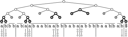
Figure 1: An illustration of Phase 1 of the algorithm, with the “cherries” depicted in thicker lines. The horizontal lines represent the LZ77-factorization and the vertical lines depict factors induced by the tree. Longer separators are drawn between chains, whose lengths are written in binary with the least significant bits on top.

Fact 22.

A block induced by a cherry is never a previous fragment. Therefore, the number of cherries is at most $z$.

Proof.

The former part follows from construction. To prove the latter, observe that the blocks induced by different cherries are disjoint and hence each cherry can be assigned a unique LZ77-factor ending within the block. ∎

Consequently, while processing level $i$ of the tree, we can afford storing all cherries generated so far on a sorted linked list $\mathcal{L}$. The remaining already generated phrases are not explicitly stored. In addition, we also store a sorted linked list $\mathcal{L}_{i}$ of all still unfactored nodes on the current level $i$ (those for which the corresponding blocks are tested as previous fragments). Their number is bounded by $z$ (because there is a cherry below every node on the list), so the total space is $\mathcal{O}(z)$. Maintaining both lists sorted is easily accomplished by scanning them in parallel with each scan of $T$, and inserting new cherries/unfactored nodes at their correct places. Furthermore, in the $i$-th round we apply Thm. 1 to at most $2^{i}$ patterns of length $n/2^{i}$, so the total time is $\sum_{i=1}^{\log n}\mathcal{O}(n+2^{i}\log(2^{i}))=\mathcal{O}(n\log n)$.

Next, we analyze the structure of the resulting factorization. Let $h_{x-1}h_{x}$ and $h_{y}h_{y+1}$ be the two consecutive cherries. The phrases $h_{x+1}\ldots h_{y-1}$ correspond to the right siblings of the ancestors of $h_{x}$ and to the left siblings of the ancestors of $h_{y}$ (no further than to the lowest common ancestor of $h_{x}$ and $h_{y}$). This naturally partitions $h_{x}h_{x+1}\ldots h_{y-1}h_{y}$ into two parts, called an increasing chain and a decreasing chain to depict the behaviour of phrase lengths within each part. Observe that these lengths are powers of two, so the structure of a chain of either type is determined by the total length of its phrases, which can be interpreted as a bitvector with bit $i^{\prime}$ set to 1 if there is a phrase of length $2^{i^{\prime}}$ in the chain. Those bitvectors can be created while traversing the tree level by level, passing the partially created bitvectors down to the next level $\mathcal{L}_{i+1}$ until finally storing them at the cherries in $\mathcal{L}$.

At the end we obtain a sequence of chains of alternating types, see Fig. 1. Since the structure of each chain follows from its length, we store the sequence of chains rather the actual factorization, which might consist of $\Theta(z\log n)=\omega(z)$ phrases. By Fact 22, our representation uses $\mathcal{O}(z)$ words of space and the last phrase of a decreasing chain concatenated with the first phrase of the consecutive increasing chain never form a previous fragment (these phrases form the block induced by the cherry).

7.1.3 Phase 2.

In this phase we merge phrases within the chains. We describe how to process increasing chains; the decreasing are handled, mutatis mutandis, analogously. We partition the phrases $h_{\ell}\ldots h_{r}$ within a chain into groups.

For each chain we maintain an active group, initially consisting of $h_{\ell}$, and scan the remaining phrases in the left-to-right order. We either append a phrase $h_{i}$ to the active group $g_{j}$, or we output $g_{j}$ and make $g_{j+1}=h_{i}$ the new active group. The former action is performed if and only if the fragment of length $2|h_{i}|$ starting at the same position as $g_{j}$ is a previous fragment. Having processed the whole chain, we also output the last active group.

Fact 23.

Within every chain every group $g_{j}$ forms a valid phrase, but no concatenation of three adjacent groups $g_{j}g_{j+1}g_{j+2}$ form a previous fragment.

Proof.

Since the lengths of phrases form an increasing sequence of powers of two, at the moment we need to decide if we append $h_{i}$ to $g_{j}$ we have $|g_{j}|\leq|h_{\ell}\ldots h_{i-1}|<|h_{i}|$, so $2|h_{i}|>|g_{j}h_{i}|$, and thus we are guaranteed if we append $g_{j}$, then $g_{j}h_{i}$ is a previous factor. Finally, let us prove the aforementioned optimality condition, i.e., that $g_{j}g_{j+1}g_{j+2}$ is not a previous fragment for any three consecutive groups. Suppose that we output $g_{j}$ while processing $h_{i}$, that is, $g_{j+1}=h_{i}\ldots h_{i^{\prime}}$. We did not append $h_{i}$ to $g_{j}$, so the fragment of length $2|h_{i}|$ starting at the same position as $g_{j}$ is not a previous fragment. However, $|g_{j}g_{j+1}g_{j+2}|>|g_{j+1}g_{j+2}|\geq|h_{i}h_{i+1}|>2|h_{i}|$, so this immediately implies that $g_{j}g_{j+1}g_{j+2}$ is not a previous fragment. ∎

The procedure described above is executed in parallel for all chains, each of which maintains just the length of its active group. In the $i$-th round only chains containing a phrase of length $2^{i}$ participate (we use bit operations to verify which chains have length containing $2^{i}$ in the binary expansion). These chains provide fragments of length $2^{i+1}$ and Thm. 1 is applied to decide which of them are previous fragments. The chains modify their active groups based on the answers; some of them may output their old active groups. These groups form phrases of the output factorization, so the space required to store them is amortized by the size of this factorization. As far as the running time is concerned, we observe that no more than $\min(z,\frac{n}{2^{i}})$ chains participate in the $i$-th round . Thus, the total running time is $\sum_{i=1}^{\log n}\mathcal{O}(n+\frac{n}{2^{i}}\log\frac{n}{2^{i}})=\mathcal{O}(n\log n)$. To bound the overall approximation guarantee, suppose there are five consecutive output phrases forming a previous fragment. By Fact 22, these fragments cannot contain a block induced by any cherry. Thus, the phrases are contained within two chains. However, by Fact 23 no three consecutive phrases obtained from a single chain form a previous fragment. Hence the resulting factorization is 5-optimal.

7.1.4 Phase 3.

The following lemma achieves the final 2-approximation:

Lemma 24.

Given a $c$-optimal factorization, one can compute a 2-optimal factorization using $\mathcal{O}(c\cdot n\log n)$ time and $\mathcal{O}(c\cdot z)$ space.

Proof.

The procedure consists of $c$ iterations. In every iteration we first detect previous fragments corresponding to concatenations of two adjacent phrases. The total length of the patterns is up to $2n$, so this takes $\mathcal{O}(n\log n+m)=\mathcal{O}(n\log n)$ time and $\mathcal{O}(c\cdot z)$ space using Thm. 12. Next, we scan through the factorization and merge every phrase $g_{i}$ with the preceding phrase $g_{i-1}$ if $g_{i-1}g_{i}$ is a previous fragment and $g_{i-1}$ has not been just merged with its predecessor.

We shall prove that the resulting factorization is 2-optimal. Consider a pair of adjacent phrases $g_{i-1}g_{i}$ in the final factorization and let $j$ be the starting position of $g_{i}$. Suppose $g_{i-1}g_{i}$ is a previous fragment. Our algorithm performs merges only, so the phrase ending at position $j-1$ concatenated with the phrase starting at position $j$ formed a previous fragment at every iteration. The only reason that these factors were not merged could be another merge of the former factor. Consequently, the factor ending at position $j-1$ took part in a merge at every iteration, i.e., $g_{i-1}$ is a concatenation of at least $c$ phrases of the input factorization. However, all the phrases created by the algorithm form previous fragments, which contradicts the $c$-optimality of the input factorization. ∎

7.2 Approximation Scheme

The starting point is a 2-optimal factorization into $a$ phrases, which can be found in $\mathcal{O}(n\log n)$ time using the previous method. The text is partitioned into $\frac{\varepsilon}{2}a$ blocks corresponding to $\frac{2}{\varepsilon}$ consecutive phrases. Every block is then greedily factorized into phrases. The factorization is implemented using Thm. 19 to compute the longest previous fragments in parallel for all blocks as follows. Denote the starting positions of the blocks by $b_{1}<b_{2}<\ldots$ and let $i_{j}$ be the current position in the $i$-th block, initially set to $b_{i}$. For every $i$, we find the longest previous fragment starting at $i_{j}$ and fully contained inside $T[i_{j}..b_{j+1}-1]$ by computing the longest prefix of $T[i_{j}..b_{j+1}-1]$ occurring in $T$ and starting in $T[1..i_{j}-1]$, denoted $T[i_{j}..i_{j}+\ell_{j}-1]$. Then we output every $T[i_{j}..i_{j}+\ell_{j}-1]$ as a new phrase and increase $i_{j}$ by $\ell_{j}$. Because every block, by definition, can be factorized into $\frac{2}{\varepsilon}$ phrases and the greedy factorization is optimal, this requires $\mathcal{O}(\frac{1}{\varepsilon}n\log n)$ time in total. To bound the approximation guarantee, observe that every phrase inside the block, except possibly for the last one, contains an endpoint of a phrase in the LZ77-factorization. Consequently, the total number of phrases is at most $z+\frac{\varepsilon}{2}a\leq(1+\varepsilon)z$.

Theorem 25.

Given a text $T$ of length $n$ whose LZ77-factorization consists of $z$ phrases, we can factorize $T$ into at most $2z$ phrases using $\mathcal{O}(n\log n)$ time and $\mathcal{O}(z)$ space. Moreover, for any $\varepsilon\in(0,1]$ in $\mathcal{O}(\varepsilon^{-1}n\log n)$ time and $\mathcal{O}(z)$ space we can compute a factorization into no more than $(1+\varepsilon)z$ phrases.

Acknowledgments.

The authors would like to thank the participants of the Stringmasters 2015 workshop in Warsaw, where this work was initiated. We are particularly grateful to Marius Dumitran, Artur Jeż, and Patrick K. Nicholson.

References

- [1] Rabin–Karp algorithm — Wikipedia, The Free Encyclopedia.
- [2] A. V. Aho and M. J. Corasick. Efficient string matching: An aid to bibliographic search. Commun. ACM, 18(6):333–340, 1975.
- [3] D. Breslauer, R. Grossi, and F. Mignosi. Simple real-time constant-space string matching. Theor. Comput. Sci., 483:2–9, 2013.
- [4] R. Clifford, A. Fontaine, E. Porat, B. Sach, and T. Starikovskaya. Dictionary matching in a stream. In N. Bansal and I. Finocchi, editors, ESA 2015, volume 8737 of LNCS, pages 361–372. Springer, Heidelberg, 2015.
- [5] M. Crochemore and D. Perrin. Two-way string matching. J. ACM, 38(3):651–675, 1991.
- [6] N. J. Fine and H. S. Wilf. Uniqueness theorems for periodic functions. P. Am. Math. Soc., 16(1):109–114, 1965.
- [7] J. Fischer, T. I, and D. Köppl. Lempel Ziv computation in small space (LZ-CISS). In F. Cicalese, E. Porat, and U. Vaccaro, editors, Combinatorial Pattern Matching - 26th Annual Symposium, CPM 2015, Ischia Island, Italy, June 29 - July 1, 2015, Proceedings, volume 9133 of Lecture Notes in Computer Science, pages 172–184. Springer, 2015.
- [8] Z. Galil and J. I. Seiferas. Time-space-optimal string matching. J. Comput. Syst. Sci., 26(3):280–294, 1983.
- [9] L. Gasieniec, M. Karpinski, W. Plandowski, and W. Rytter. Efficient algorithms for Lempel-Ziv encoding (extended abstract). In R. G. Karlsson and A. Lingas, editors, SWAT 1996, volume 1097 of LNCS, pages 392–403. Springer, Heidelberg, 1996.
- [10] B. Gum and R. J. Lipton. Cheaper by the dozen: Batched algorithms. In V. Kumar and R. L. Grossman, editors, SDM 2001, pages 1–11. SIAM, Philadelphia, 2001.
- [11] W. Hon, T. Ku, R. Shah, S. V. Thankachan, and J. S. Vitter. Faster compressed dictionary matching. Theor. Comput. Sci., 475:113–119, 2013.
- [12] J. Kärkkäinen, D. Kempa, and S. J. Puglisi. Lightweight Lempel-Ziv parsing. In V. Bonifaci, C. Demetrescu, and A. Marchetti-Spaccamela, editors, SEA 2013, volume 7933 of LNCS, pages 139–150. Springer, Heidelberg, 2013.
- [13] R. M. Karp and M. O. Rabin. Efficient randomized pattern-matching algorithms. IBM J. Res. Dev., 31(2):249–260, 1987.
- [14] T. Kociumaka, T. Starikovskaya, and H. W. Vildhøj. Sublinear space algorithms for the longest common substring problem. In A. S. Schulz and D. Wagner, editors, ESA 2014, volume 8737 of LNCS, pages 605–617. Springer, Heidelberg, 2014.
- [15] M. Lohrey. Algorithmics on SLP-compressed strings: A survey. Groups Complexity Cryptology, 4(2):241–299, 2012.
- [16] M. Ružić. Constructing efficient dictionaries in close to sorting time. In L. Aceto, I. Damgård, L. A. Goldberg, M. M. Halldórsson, A. Ingólfsdóttir, and I. Walukiewicz, editors, ICALP 2008, volume 5125, pages 84–95. Springer, Heidelberg, 2008.
- [17] E. Ukkonen. On-line construction of suffix trees. Algorithmica, 14(3):249–260, 1995.
- [18] J. Ziv and A. Lempel. A universal algorithm for sequential data compression. IEEE Trans. Inform. Theory, 23(3):337–343, 1977.