ADMM Algorithmic Regularization Paths for Sparse Statistical Machine Learning

Abstract

Optimization approaches based on operator splitting are becoming popular for solving sparsity regularized statistical machine learning models. While many have proposed fast algorithms to solve these problems for a single regularization parameter, conspicuously less attention has been given to computing regularization paths, or solving the optimization problems over the full range of regularization parameters to obtain a sequence of sparse models. In this chapter, we aim to quickly approximate the sequence of sparse models associated with regularization paths for the purposes of statistical model selection by using the building blocks from a classical operator splitting method, the Alternating Direction Method of Multipliers (ADMM). We begin by proposing an ADMM algorithm that uses warm-starts to quickly compute the regularization path. Then, by employing approximations along this warm-starting ADMM algorithm, we propose a novel concept that we term the ADMM Algorithmic Regularization Path. Our method can quickly outline the sequence of sparse models associated with the regularization path in computational time that is often less than that of using the ADMM algorithm to solve the problem at a single regularization parameter. We demonstrate the applicability and substantial computational savings of our approach through three popular examples, sparse linear regression, reduced-rank multi-task learning, and convex clustering.

1 Introduction

With the rise of Big Data and the subsequent explosion of statistical machine learning methods to analyze it, statisticians have become avid consumers of large-scale optimization procedures to estimate sparse models. The estimation problem is often cast as an optimization problem of the form:

$$\underset{\operatorname{\bm{\beta}}}{\text{minimize}}\quad L(\operatorname{\bm{\beta}};\mathbf{W})+\lambda P(\operatorname{\bm{\beta}}),$$ (1)

where $\operatorname{\bm{\beta}}$ is a parameter which specifies a statistical model, $L(\operatorname{\bm{\beta}};\mathbf{W})$ is a smooth loss function or data-fidelity term that quantifies the discrepancy between the data, $\mathbf{W}$, and the model specified by $\operatorname{\bm{\beta}}$, and $P(\operatorname{\bm{\beta}})$ is a nonsmooth penalty that encourages sparsity in model parameter $\operatorname{\bm{\beta}}$ boyd2011distributed ; buhlmann2011statistics ; hastie2009elements . A regularization parameter, $\lambda\geq 0$, explicitly trades off the model fit and the model complexity.

Directly solving the optimization problem (1) is often challenging. Operator splitting methods, such as the Alternating Direction Method of Multipliers (ADMM), have become popular because they convert solving the problem into solving a sequence of simpler optimization problems that involve only the smooth loss or nonsmooth penalty. By breaking up the problem into smaller ones, ADMM may end up taking more iterations than directly solving (1), but it often runs in less total time since the subproblems are typically easy to solve. Clearly in the context of Big Data, faster algorithms are indispensable, and the numerical optimization community has devoted a great deal of effort to solving (1) rapidly for a fixed value of $\lambda$. This goal, however, is not necessarily aligned with the application of statistical machine learning problems to real data.

In practice, statisticians are interested in finding the best sparse model that represents the data. Achieving this typically entails a two-step procedure: (i) model selection, or selecting the best sparse model or equivalently the best subset of parameters, and (ii) model fitting, or fitting the model by minimizing the loss function over the selected parameters hastie2009elements . The first step is often the most challenging computationally as this entails searching the combinatorial space of all possible sparse models. As this combinatorial search is infeasible for large-scale problems, many consider convex relaxations through constraints or penalties as computationally feasible surrogates to help search through the space of sparse models. Consider for example, sparse linear regression, where the goal is to find the subset of variables or inputs that best predicts the response or output. Searching over all possible subsets of variables, however, is an NP hard problem. Instead, many have employed the penalty or constraint, $P(\operatorname{\bm{\beta}})=\lVert\operatorname{\bm{\beta}}\rVert_{1}$, which is the tightest convex relaxation to performing best subset selection and whose solution can be computed in polynomial time. The nonsmooth penalty term, $P(\operatorname{\bm{\beta}})$, then serves to translate an infeasible computational problem into a tractable one for model selection purposes.

Suppose now that we focus on selecting the best sparse model by means of penalized statistical estimation as in (1). As $\lambda$ varies, we trace out a continuous parametric curve $\hat{\operatorname{\bm{\beta}}}(\lambda)\in\mathbb{R}^{p}$. Since this curve cannot be determined analytically in general, the curve is estimated for a finite sequence of regularization parameters. To choose the best model, statisticians inspect the sequence of sparse solutions to (1) over the full range of regularization parameters: $\{\hat{\operatorname{\bm{\beta}}}(\lambda_{n}):0\leq\lambda_{1}\leq\cdots\leq\lambda_{\max}\}$, where $\lambda_{\max}$ is the value of $\lambda$ at which $\hat{\operatorname{\bm{\beta}}}(\lambda_{\max})=\mathbf{0}$, the maximally sparse solution. This sequence of sparse solutions is often called the regularization path friedman2007pathwise ; friedman2010regularization ; hastie2004entire . For model selection purposes, however, the actual parameter values, $\hat{\operatorname{\bm{\beta}}}(\lambda)$, as $\lambda$ varies in the regularization paths are less important than identifying the non-zero components of $\hat{\operatorname{\bm{\beta}}}(\lambda)$. (Note that the parameter values for the optimal model are typically re-fit anyways in the second model fitting stage.) Instead, the support of $\hat{\operatorname{\bm{\beta}}}(\lambda)$ or the sequence of active sets defined as $\mathcal{A}(\lambda)=\{j:\hat{\beta}_{j}(\lambda)\neq 0\}$, are the important items; these yield a good sequence of sparse models to consider that limit computationally intensive exploration of a combinatorial model space. Out of this regularization path or sequence of active sets, the optimal model can be chosen via a number of popular techniques such as minimizing the trade-off in model complexity as with the AIC and BIC, the prediction error as with cross-validation hastie2009elements or the model stability as with stability selection meinshausen2010stability .

To apply sparse statistical learning methods to large-scale problems, we need fast algorithms not only to fit (1) for one value of $\lambda$, but to estimate the entire sequence of sparse models in the model selection stage. Our objective in this chapter is to study the latter, which has received relatively little attention from the optimization community. Specifically, we seek to develop a new method to approximate the sequence of active sets associated with regularization paths that is (i) computationally fast and (ii) comprehensively explores the space of sparse models at a sufficiently fine resolution. In doing so, we will not try to closely approximate the parameter values, $\hat{\operatorname{\bm{\beta}}}(\lambda)$, but instead try to closely approximate the sparsity of the parameters, $\mathcal{A}(\lambda)$, for the statistical learning problem (1).

To rapidly approximate the sequence of active sets associated with regularization paths, we turn to the ADMM optimization framework. We first introduce a procedure to estimate the regularization path by using the ADMM algorithm with warm starts over a range of regularization parameters to yield a path-like sequence of solutions. Extending this, we preform a one-step approximation along each point on this path, yielding the novel method that we term ADMM Algorithmic Regularization Paths. Our procedure can closely approximate active sets given by regularization paths at a fine resolution, but dramatically reduces computational time. This new approach to estimating a sequence of sparse models opens many interesting questions from both statistical and optimization perspectives. In this chapter, however, we focus on motivating our approach and demonstrating its computational advantages on several sparse statistical machine learning examples.

This chapter is organized as follows. We first review how ADMM algorithms have been used in the statistical machine learning literature, Section 1.1. Then, to motivate our approach, we consider application of ADMM to the familiar example of sparse linear regression, Section 1.2. In Section 2, we introduce our novel Algorithmic Regularization Paths for general sparse statistical machine learning procedures. We then demonstrate how to apply our methods through some popular machine learning problems in Section 3; specifically, we consider three examples – sparse linear regression (Section 3.1), reduced-rank multi-task learning (Section 3.2), and convex clustering (Section 3.3) – where our Algorithm Paths yield substantial computational benefits. We conclude with a discussion of our work and the many open questions it raises in Section 4.

1.1 ADMM in Statistical Machine Learning

The ADMM algorithm has become popular in statistical machine learning in recent years because the resulting algorithms are typically simple to code and can scale efficiently to large problems. Although ADMM has been successfully applied over a diverse spectrum of problems, there are essentially two thematic challenges among the problems that ADMM has proven adept at addressing: (i) decoupling constraints and regularizers, that are straightforward to handle individually, but not in conjunction; and (ii) simplifying fusion type penalties. We make note of these two types of problems because the ADMM Algorithmic Regularization Path we introduce in this chapter can be applied to either type of problem.

An illustrative example of the first thematic challenge arises in sparse principal component analysis (PCA). In VuChoLei2013 Vu et al. propose estimating sparse principal subspace estimator ${\bm{\hat{\mathbf{{B}}}}}$ of a symmetric input matrix ${\bm{\mathbf{{S}}}}$ with the solution to the following semidefinite program:

$$\underset{\operatorname{\mathbf{B}}}{\text{minimize}}\quad-\langle{\bm{\mathbf{{S}}}},{\bm{\mathbf{{B}}}}\rangle+\lambda\lVert{\bm{\mathbf{{B}}}}\rVert_{1}\quad\text{subject to}\quad{\bm{\mathbf{{B}}}}\in\mathcal{F}^{d},$$

where $\lVert{\bm{\mathbf{{B}}}}\rVert_{1}$ is 1-norm of the vectorization of ${\bm{\mathbf{{B}}}}$, the set $\mathcal{F}^{d}=\{{\bm{\mathbf{{B}}}}:{\bm{\mathbf{{0}}}}\preceq{\bm{\mathbf{{B}}}}\preceq{\bm{\mathbf{{I}}}},\operatorname{tr}({\bm{\mathbf{{B}}}})=d\}$ is a closed and convex set called the Fantope, and $\lambda\geq 0$ is a regularization parameter. The main algorithmic challenge is the interaction between the Fantope constraint and the $\ell_{1}$-norm penalty. If only either the penalty or constraint were present the problem would be straightforward to solve. Consider the following equivalent problem to which ADMM can be readily applied:

$$\underset{\operatorname{\mathbf{B}}}{\text{minimize}}\quad\delta_{\mathcal{F}^{d}}({\bm{\mathbf{{B}}}})-\langle{\bm{\mathbf{{S}}}},{\bm{\mathbf{{B}}}}\rangle+\lambda\lVert{\bm{\mathbf{{Z}}}}\rVert_{1}\quad\text{subject to}\quad{\bm{\mathbf{{Z}}}}-{\bm{\mathbf{{B}}}}={\bm{\mathbf{{0}}}},$$

where $\delta_{C}(\bm{\Sigma})$ denotes the indicator function of the closed convex set $C$, namely the function that is $0$ on $C$ and $\infty$ otherwise. By minimizing an augmented Lagrangian over ${\bm{\mathbf{{B}}}}$, the copy variable ${\bm{\mathbf{{Z}}}}$, and the scaled dual variable ${\bm{\mathbf{{U}}}}$ as outlined in boyd2011distributed , we arrive at the following ADMM updates:

$${\bm{\mathbf{{B}}}}^{k} = \underset{{\bm{\mathbf{{B}}}}}{\arg\min}\;\frac{1}{2}\lVert{\bm{\mathbf{{B}}}}-({\bm{\mathbf{{Z}}}}^{k-1}-{\bm{\mathbf{{U}}}}^{k-1}+\rho^{-1}{\bm{\mathbf{{S}}}})\rVert_{\text{F}}^{2}+\delta_{\mathcal{F}^{d}}({\bm{\mathbf{{B}}}})=\mathcal{P}_{\mathcal{F}^{d}}({\bm{\mathbf{{Z}}}}^{k-1}-{\bm{\mathbf{{U}}}}^{k-1}+\rho^{-1}{\bm{\mathbf{{S}}}})$$

$${\bm{\mathbf{{Z}}}}^{k} = \underset{{\bm{\mathbf{{Z}}}}}{\arg\min}\;\frac{\lambda}{\rho}\lVert{\bm{\mathbf{{Z}}}}\rVert_{1}+\frac{1}{2}\lVert{\bm{\mathbf{{B}}}}^{k}+{\bm{\mathbf{{U}}}}^{k-1}-{\bm{\mathbf{{Z}}}}\rVert_{\text{F}}^{2}=S_{\lambda/\rho}({\bm{\mathbf{{B}}}}^{k}+{\bm{\mathbf{{U}}}}^{k-1})$$

$${\bm{\mathbf{{U}}}}^{k} = {\bm{\mathbf{{U}}}}^{k-1}+{\bm{\mathbf{{B}}}}^{k}-{\bm{\mathbf{{Z}}}}^{k}.$$

Thus, the penalty and constraint are effectively decoupled resulting in simple updates: the update for ${\bm{\mathbf{{Z}}}}$ requires the soft-thresholding operator, $S_{\mu}(\operatorname{\mathbf{x}})=\operatorname{sign}({\operatorname{\mathbf{x}}})(\lvert\operatorname{\mathbf{x}}\rvert-\mu)_{+}$, and the update for ${\bm{\mathbf{{B}}}}$ involves the projection onto the Fantope, denoted by $\mathcal{P}_{\mathcal{F}^{d}}$, which has a closed form solution given in VuChoLei2013 .

The literature abounds with many more examples of using the ADMM splitting strategy to decouple an otherwise challenging optimization problem into simpler subproblems. Boyd et al. boyd2011distributed review many such applications. Other example applications include decoupling trace or nuclear norm penalties as in robust PCA YuaYan2012 , latent variable graphical models MaXue2013 , and tensor completion liu2009tensor ; decoupling different types of hierarchical constraints bien2013lasso , decoupling a series of loss functions hu2014local , decoupling joint graphical models DanWan2014 , and decoupling large linear programming problems AguXinSmi2011 , among many others.

The second thematic challenge that ADMM algorithms have been used to solve involve fusion or non-separable penalties. A good illustrative example of this challenge arises in total variation (TV) denoising RudOshFat1992 . Consider the simple version of this problem, specifically finding a smooth estimate of a noisy one-dimensional signal $y\in\Re^{n}$:

$$\underset{\operatorname{\bm{\beta}}}{\text{minimize}}\quad\frac{1}{2}\lVert{\bm{\mathbf{{y}}}}-\operatorname{\bm{\beta}}\rVert_{2}^{2}+\lambda\sum_{i=1}^{n-1}\lvert{\beta}_{i}-{\beta}_{i+1}\rvert,$$

where the tuning parameter $\lambda\geq 0$ trades off the smoothness of the approximation with the goodness of fit with the data ${\bm{\mathbf{{y}}}}$. What makes this problem challenging is that the fusion penalty couples the non-smooth terms so that they are non-separable. Note that this penalty can be written more compactly as $\rVert\mathbf{A}\operatorname{\mathbf{x}}\lVert_{1}$ where ${\bm{\mathbf{{A}}}}$ is the discrete first order differences operator matrix. More generally, this second class of problems consist of problems of the form, $L(\operatorname{\bm{\beta}};\mathbf{W})+\lambda P({\bm{\mathbf{{A}}}}\operatorname{\bm{\beta}})$. In the machine learning context these penalties arise because we often wish to impose structure, not on a latent variable of interest directly, but rather on a linear transformation of it. In the TV denoising example we seek sparsity in differences of adjacent time points of the latent signal.

Previously, we could break the objective into a sum of simpler objectives. The issue here is different; specifically the composition of the regularizer with a linear mapping complicates matters. ADMM can again greatly simplify this problem if we let the ADMM copy variable copy the linearly transformed parameters:

$$\underset{\operatorname{\bm{\beta}}}{\text{minimize}}\quad L(\operatorname{\bm{\beta}};\mathbf{W})+\lambda P({\bm{\mathbf{{z}}}})\quad\text{subject to}\quad{\bm{\mathbf{{z}}}}-{\bm{\mathbf{{A}}}}{\bm{\mathbf{{\operatorname{\bm{\beta}}}}}}={\bm{\mathbf{{0}}}}.$$

The ADMM subproblems for iteratively solving this problem then have the following simple form:

$${\bm{\mathbf{{\operatorname{\bm{\beta}}}}}}^{k} = \underset{\operatorname{\bm{\beta}}}{\arg\min}\;\ \ L(\operatorname{\bm{\beta}};\mathbf{W})+\frac{\rho}{2}\lVert{\bm{\mathbf{{A}}}}\operatorname{\bm{\beta}}-{\bm{\mathbf{{z}}}}^{k-1}+{\bm{\mathbf{{u}}}}^{k-1}\rVert_{2}^{2}$$

$${\bm{\mathbf{{z}}}}^{k} = \underset{{\bm{\mathbf{{z}}}}}{\arg\min}\;\ \ P({\bm{\mathbf{{z}}}})+\frac{\rho}{2}\lVert{\bm{\mathbf{{z}}}}-{\bm{\mathbf{{A}}}}{\bm{\mathbf{{\operatorname{\bm{\beta}}}}}}^{k}-{\bm{\mathbf{{u}}}}^{k-1}\rVert_{2}^{2}$$

$${\bm{\mathbf{{u}}}}^{k} = {\bm{\mathbf{{u}}}}^{k-1}+{\bm{\mathbf{{\operatorname{\bm{\beta}}}}}}^{k}-{\bm{\mathbf{{z}}}}^{k}.$$

Note that we have eliminated having to minimize any functions containing the troublesome composition penalty. In the context of the TV denoising example, the $\operatorname{\bm{\beta}}$ update requires solving a linear system of equations, and the ${\bm{\mathbf{{z}}}}$ update involves a straightforward soft-threshold.

The ADMM algorithm has been used to decouple fusion or non-separable types of penalties in many statistical learning problems. These include more general instances of total variation wahlberg2012admm ; GolOsh2009 , a convex formulation of clustering ChiLan2013 , joint graphical model selection MohChuHan2012 ; MohLonFaz2014 , overlapping group lasso penalties yuan2011efficient , and more generally for structured sparsity mairal2011convex .

Overall, while the ADMM algorithm is gaining more widespread application in statistics and machine learning, the algorithm is applied in the traditional sense to solve a composite optimization problem for one value of the regularization parameter. In this chapter, we seek to investigate the ADMM algorithm for a different purpose, namely to find a sequence of sparse models associated with regularization paths.

1.2 Developing an Algorithmic Regularization Path: Sparse Regression

Our goal is to quickly generate a sequence of candidate sparse solutions for model selection purposes. To achieve this, we will propose a method of approximating the sequence of active sets given by regularization paths, or the path-like sequence solutions of penalized statistical models over the full range of regularization parameters. To motivate our approach, we study the familiar example of sparse linear regression. Suppose we observe a covariate matrix $\operatorname{\mathbf{X}}\in\Re^{n\times p}$ consisting of $n$ iid observations of $p$ variables and an associated response variable $\operatorname{\mathbf{y}}\in\Re^{n}$. We are interested in fitting the linear model $\operatorname{\mathbf{y}}=\operatorname{\mathbf{X}}\operatorname{\bm{\beta}}+\epsilon$ where $\epsilon$ is independent noise, but assume that the linear coefficient vector $\operatorname{\bm{\beta}}$ is sparse, $\rVert\operatorname{\bm{\beta}}\lVert_{0}\ll p$ where $\lVert\cdot\rVert_{0}$ is the $\ell_{0}$ norm or the number of non-zero elements of $\operatorname{\bm{\beta}}$. Minimizing a criterion subject to a constraint of the form $\lVert\operatorname{\bm{\beta}}\rVert_{0}\leq k$ for some $k$, becomes a combinatorially hard task. To estimate a sparse model in reasonable time, many have proposed to use the tightest convex relaxation, the $\ell_{1}$-norm penalty, commonly called the LASSO tibshiranit1996regression in the statistical literature:

$$\underset{\operatorname{\bm{\beta}}}{\text{minimize}}\quad\frac{1}{2n}\lVert\operatorname{\mathbf{y}}-\operatorname{\mathbf{X}}\operatorname{\bm{\beta}}\rVert_{2}^{2}+\lambda\lVert\operatorname{\bm{\beta}}\rVert_{1}$$ (2)

where $\lambda\geq 0$ is the regularization parameter controlling the sparsity of $\operatorname{\bm{\beta}}$.

The full regularization path of solutions for the LASSO is the set of regression coefficients $\{\hat{\operatorname{\bm{\beta}}}(\lambda):\ \forall\ 0\leq\lambda\leq\lambda_{\max}\}$ where $\lambda_{\max}=\frac{1}{n}\lVert\operatorname{\mathbf{X}}^{\sf T}\operatorname{\mathbf{y}}\rVert_{\infty}$ is the smallest amount of regularization that yields the sparse solution $\hat{\operatorname{\bm{\beta}}}=\mathbf{0}$. The regularization paths for the LASSO have been well-studied and in particular, are continuous and piece-wise linear osborne2000new ; efron2004least ; rosset2007piecewise . These paths also outline a sequence of active sets or sparse models that smoothly increase in sparsity levels as $\lambda$ decreases from the fully sparse solution at $\lambda=\lambda_{\max}$ to the fully dense solution at $\lambda=0$. Hence for model selection, one can limit exploration of the combinatorial space of sparse models to that of the sequence of active sets outlined by the LASSO regularization paths.

Computing the full regularization paths, however, can be a computational challenge. Several path following algorithms for the LASSO osborne2000new ; rosset2007piecewise and closely related algorithms such as such as Least Angle Regression (LAR) efron2004least and Orthogonal Matching Pursuit (OMP) donoho2012sparse have been proposed; their computational complexity, however, is $\mathcal{O}(p^{3})$ which is prohibitive for large-scale problems. Consequently, many have suggested to closely approximate these paths by solving a series of optimization problems over a grid of regularization parameter values. Specifically, this is typically done for a sequence of 100 log-spaced values from $\lambda_{\max}$ to $\lambda_{1}=0$. Statisticians often employ homotopy, or warm-starts, to speed computation along the regularization path friedman2007pathwise . Warm-starts use the solution from the previous value of $\lambda_{j}$, $\hat{\operatorname{\bm{\beta}}}(\lambda_{j})$, as the initialization for the optimization algorithm to solve the problem at $\lambda_{j+1}$. As the coefficients, $\operatorname{\bm{\beta}}$, change continuously in $\lambda$, warm-starts can dramatically reduce the number of iterations needed for convergence as $\hat{\operatorname{\bm{\beta}}}(\lambda_{j})$ is expected to be close to $\hat{\operatorname{\bm{\beta}}}(\lambda_{j+1})$ for small changes from $\lambda_{j}$ to $\lambda_{j+1}$. Many consider shooting methods, or coordinate descent procedures friedman2007pathwise ; wu2008coordinate , that use warm-starts and iterate over the active set for 100 log-spaced values of $\lambda$ friedman2010regularization to be the fastest approximate solvers of the LASSO regularization path.

We seek to further speed the computation of the sequence of active sets given by the regularization path by using a single path approximating algorithm instead of solving separate optimization problems over a grid of regularization parameter values. Our approach is motivated by two separate observations: (i) the evolution of the sparsity level of the iterates of the ADMM algorithm used to fit (2) for one value of $\lambda$, and (ii) the behavior of a new version of the ADMM algorithm that incorporates warm-starts to expedite computation of regularization paths. We study each of these motivations separately, beginning with the first.

Consider using ADMM to solve the LASSO problem. First, we split the differentiable loss function from the non-differentiable penalty term by introducing a copy $\operatorname{\mathbf{z}}$ of the variable $\operatorname{\bm{\beta}}$ in the penalty function, and adding an equality constraint forcing them to be equal. The LASSO problem (2) can then be re-written as:

$$\underset{\operatorname{\bm{\beta}},\operatorname{\mathbf{z}}}{\text{minimize}}\quad\frac{1}{2n}\lVert\operatorname{\mathbf{y}}-\operatorname{\mathbf{X}}\operatorname{\bm{\beta}}\rVert_{2}^{2}+\lambda\lVert\operatorname{\mathbf{z}}\rVert_{1}\quad\text{subject to}\quad\operatorname{\bm{\beta}}=\operatorname{\mathbf{z}},$$

with its associated augmented Lagrangian:

$$\mathcal{L}(\operatorname{\bm{\beta}},\operatorname{\mathbf{z}},\operatorname{\mathbf{u}})=\frac{1}{2n}\lVert\operatorname{\mathbf{y}}-\operatorname{\mathbf{X}}\operatorname{\bm{\beta}}\rVert_{2}^{2}+\lambda\lVert\operatorname{\mathbf{z}}\rVert_{1}+\frac{\rho}{2}\lVert\operatorname{\bm{\beta}}-\operatorname{\mathbf{z}}+\operatorname{\mathbf{u}}\rVert_{2}^{2}.$$

Here, $\operatorname{\mathbf{u}}$ is the scaled dual variable of the same dimension as $\operatorname{\bm{\beta}}$ and $\rho$ is the algorithm tuning parameter. The ADMM algorithm then follows three steps (subproblems) to solve the LASSO:

$$\operatorname{\bm{\beta}}\text{-subproblem: }\operatorname{\bm{\beta}}^{k}=\underset{\operatorname{\bm{\beta}}}{\arg\min}\;\frac{1}{2n}\lVert\operatorname{\mathbf{y}}-\operatorname{\mathbf{X}}\operatorname{\bm{\beta}}\rVert_{2}^{2}+\frac{\rho}{2}\lVert\operatorname{\bm{\beta}}-\operatorname{\mathbf{z}}^{k-1}+\operatorname{\mathbf{u}}^{k-1}\rVert_{2}^{2}$$

$$\operatorname{\mathbf{z}}\text{-subproblem: }\operatorname{\mathbf{z}}^{k}=\underset{\operatorname{\mathbf{z}}}{\arg\min}\;\lambda\lVert\operatorname{\mathbf{z}}\rVert_{1}+\frac{\rho}{2}\lVert\operatorname{\mathbf{z}}-\operatorname{\bm{\beta}}^{k}-\operatorname{\mathbf{u}}^{k-1}\rVert_{2}^{2}$$

$$\text{Dual update: }\operatorname{\mathbf{u}}^{k}=\operatorname{\mathbf{u}}^{k-1}+\operatorname{\bm{\beta}}^{k}-\operatorname{\mathbf{z}}^{k}.$$

The benefit of solving this reformulation is simpler iterative updates. These three steps are iterated until convergence, typically measured by the primal and dual residuals boyd2011distributed . The $\operatorname{\bm{\beta}}$-subproblem solves a linear regression with an additional quadratic ridge penalty. Solving the $\operatorname{\mathbf{z}}$-subproblem introduces sparsity. Notice that this is the proximal operator of the $\ell_{1}$-norm applied to $\operatorname{\bm{\beta}}^{k}-\operatorname{\mathbf{u}}^{k}$ which is solved analytically via soft-thresholding.Finally, the dual update ensures that $\operatorname{\bm{\beta}}$ is squeezed towards $\operatorname{\mathbf{z}}$ and primal feasibility as the algorithm progresses.

Consider the sparsity of the $\operatorname{\mathbf{z}}$ iterates, $\lVert\operatorname{\mathbf{z}}^{k}\rVert_{0}$, for the LASSO problem. Notice that as the algorithm proceeds, $\operatorname{\mathbf{z}}^{k}$ becomes increasingly sparse; this is illustrated for a small simulated example in the left panel of Figure 1. Let us study why this occurs and its implications. Regardless of $\lambda$, the ADMM algorithm begins with a fully dense $\operatorname{\bm{\beta}}^{1}$ as this is the solution to a ridge problem with parameter $\rho$. Soft-thresholding in the $\operatorname{\mathbf{z}}$-subproblem then sets coefficients of small magnitude to zero. The first dual update, $\operatorname{\mathbf{u}}^{1}$, has magnitude at most $|\lambda|$, meaning that the second $\operatorname{\bm{\beta}}^{2}$ update is essentially shrunken towards $\operatorname{\bm{\beta}}^{1}$. Smaller coefficients decrease further in magnitude and soft-thresholding in the $\operatorname{\mathbf{z}}$-subproblem sets even more coefficients to zero. The algorithm thus proceeds until the sparsity of the $\operatorname{\mathbf{z}}^{k}$ stabilizes to that of the solution, $\hat{\operatorname{\bm{\beta}}}(\lambda)$. Hence, the support of the $\operatorname{\mathbf{z}}^{k}$ has approximated the active set of the solution long before the iterates of the $\operatorname{\bm{\beta}}$-subproblem; the latter typically does not reach the sparsity of the solution until convergence when primal feasibility is achieved. While Figure 1 only illustrates that $\operatorname{\mathbf{z}}^{k}$ quickly converges to the correct sparsity level, we have observed empirically in all our examples that the active set outlined by $\lVert\operatorname{\mathbf{z}}^{k}\rVert_{0}$ also quickly identifies the true non-zero elements of the solution, $\hat{\operatorname{\bm{\beta}}}(\lambda)$.

Interestingly then, the $\operatorname{\mathbf{z}}^{k}$ quickly explore a sequence of sparse models going from dense to sparse, similar in nature to the sequence of sparse models outlined by the regularization path. While from Figure 1 we can see that this sequence of sparse models is not desirable as it does not smoothly transition in sparsity and does not fully explore the sparse model space, we nonetheless learn two important items from this: (i) We are motivated to

consider using the algorithm iterates of the $\operatorname{\mathbf{z}}$-subproblem, as a possible means of quickly exploring the sparse model space; and (ii) we are motivated to consider a sequence of solutions going from dense to sparse as this naturally aligns with the sparsity levels observed in the ADMM algorithm iterates. Given these, we ask: Is it possible to use or modify the iterates of the ADMM algorithm to achieve a path-like smooth transition in sparsity levels similar in nature to the sparsity levels and active sets corresponding to regularization paths?

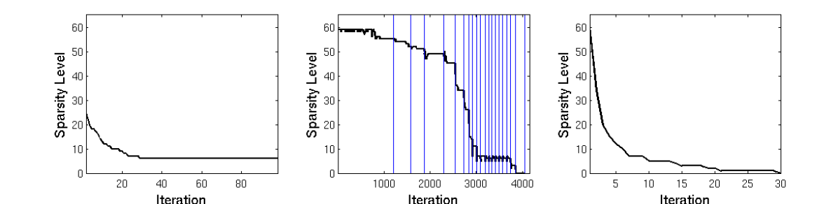
Figure 1: Sparsity levels outlining a sequence of active sets for a simulated sparse linear regression example. (Left) Sparsity levels of the $\operatorname{\mathbf{z}}$-subproblem iterates of the ADMM algorithm, $\lVert\operatorname{\mathbf{z}}^{k}\rVert_{0}$, fit for one fixed value of $\lambda$. (Middle) Sparsity levels of the $\operatorname{\mathbf{z}}$-subproblem over the iterates of our path approximating ADMM Algorithm with Warm Starts for a small range of $\bm{\lambda}$. Vertical lines denote the start of the algorithm for an increased value of $\lambda$. (Right) Sparsity levels of the $\operatorname{\mathbf{z}}$-subproblem over the iterates of our novel ADMM Algorithmic Regularization Path.

One possible solution would be to employ warm-starts in the ADMM algorithm along a grid of regularization parameters similar to other popular algorithms for approximating regularization paths. Recall that warm-starts use the solution obtained at the previous value of $\lambda$ as initialization for the next value of $\lambda$. We first introduce this new extension of the ADMM algorithm for approximating regularization paths in Algorithm 1 and then return to our motivation of studying the sequence of active sets outlined by this algorithm.

Algorithm 1 ADMM with Warm Starts: Sparse Regression

1. Initialize $\operatorname{\bm{\beta}}^{0}=\operatorname{\mathbf{0}}$, $\operatorname{\mathbf{u}}^{0}=\operatorname{\mathbf{0}}$, and $M$ log-spaced values, $\bm{\lambda}=\{\lambda_{1}<\lambda_{2}<\ldots<\lambda_{M}\}$, for $\lambda_{1}=0$ and $\lambda_{M}=\lambda_{\max}$.

2. Precompute matrix inverse $\operatorname{\mathbf{H}}=(\operatorname{\mathbf{X}}^{\sf T}\operatorname{\mathbf{X}}/n+\operatorname{\mathbf{I}})^{-1}$ and $\operatorname{\mathbf{H}}\operatorname{\mathbf{X}}^{\sf T}\operatorname{\mathbf{y}}$.

3. for $j=1\ldots M$ do

        while  $\lVert\mathbf{r}^{k}\rVert\wedge\lVert\mathbf{s}^{k}\rVert>\epsilon^{\text{tol}}$ do

            $\operatorname{\mathbf{z}}_{j}^{k}=S_{\lambda_{j}}(\operatorname{\bm{\beta}}_{j}^{k-1}+\operatorname{\mathbf{u}}_{j}^{k-1})$

            $\operatorname{\bm{\beta}}_{j}^{k}=\operatorname{\mathbf{H}}\operatorname{\mathbf{X}}^{\sf T}\operatorname{\mathbf{y}}+\operatorname{\mathbf{H}}(\operatorname{\mathbf{z}}_{j}^{k}-\operatorname{\mathbf{u}}_{j}^{k-1})$

            $\operatorname{\mathbf{u}}_{j}^{k}=\operatorname{\mathbf{u}}^{k-1}+\operatorname{\bm{\beta}}_{j}^{k}-\operatorname{\mathbf{z}}_{j}^{k}$

            $\mathbf{r}^{k}=\operatorname{\bm{\beta}}_{j}^{k}-\operatorname{\mathbf{z}}_{j}^{k}$ and $\mathbf{s}^{k}=\operatorname{\mathbf{z}}_{j}^{k}-\operatorname{\mathbf{z}}_{j}^{k-1}$

            $k=k+1$

        end while

   end for

4. Output $\{\operatorname{\bm{\beta}}_{j}:j=1,\cdots,M\}$ as the regularization path.

Our ADMM algorithm with warm starts is an alternative algorithm for fitting regularization paths. It begins with $\lambda$ small corresponding to a dense model, fits the ADMM algorithm to obtain the solution, and then uses the previous solution, $\operatorname{\bm{\beta}}(\lambda_{j-1})$, and dual variable, $\operatorname{\mathbf{u}}(\lambda_{j-1})$, to initialize the ADMM algorithm for $\lambda_{j}$.

Before considering the sequence of active sets outlined by this algorithm, we pause to discuss some noteworthy features. First, notice that the ADMM tuning parameter, $\rho$, does not appear in this algorithm. We have omitted this as a parameter by fixing $\rho=1$ throughout the algorithm. Fixing $\rho$ stands in contrast with the burgeoning literature on how to dynamically update $\rho$ for ADMM algorithms boyd2011distributed . For example, adaptive procedures that change $\rho$ to speed up convergence are introduced in he2000alternating . Others have proposed accelerated versions of the ADMM algorithm that achieve a similar phenomenon goldstein2012fast . Changing the algorithm tuning parameter, however, is not conducive to achieving a path-like algorithm using warm-starts. Consider the $\operatorname{\mathbf{z}}$-subproblem which is solving by soft-thresholding at the level $\lambda_{j}/\rho$. Thus, if $\rho$ is changed in the algorithm, the sparsity levels of $\operatorname{\mathbf{z}}$ dramatically change, eliminating the advantages of using warm-starts to achieve smooth transitions in sparsity levels. Second, notice that we have switched the order of the sub-problems by beginning with the $\operatorname{\mathbf{z}}$-subproblem. While technically the order of the subproblems does not matter yan2014self , we begin with the $\operatorname{\mathbf{z}}$-subproblem as this is where the sparsity is achieved through soft-thresholding at the value, $\lambda$; hence, the solution for $\operatorname{\mathbf{z}}$ is what changes when $\lambda$ is increased.

Next, notice that our regularization paths go from dense to sparse, or $\lambda$ small to large, which is the opposite of other path-wise algorithms and algorithms that approximate regularization paths over a grid of $\lambda$ values friedman2010regularization . Recall that our objective is to obtain a smooth path-like transition in sparsity levels corresponding to a sequence of active sets that fully explores the space of sparse models. Our warm-start procedure naturally aligns with the sparsity levels of the iterates of the ADMM algorithm which go from dense to sparse, thus ensuring a smooth transition in the sparsity level of $\operatorname{\mathbf{z}}$ as $\lambda$ is increased. Our warm-start procedure could certainly be employed going in the reverse direction from sparse to dense, but we have observed that this introduces discontinuities in the $\operatorname{\mathbf{z}}^{k}$ iterates and consequently their active sets as well, thus requiring more iterations for convergence. This behavior occurs as the solution of the $\operatorname{\bm{\beta}}$-subproblem is always more dense than that of the $\operatorname{\mathbf{z}}$-subproblem, even when employing warm-starts.

Now, let us return to our motivation and consider the sparsity levels and corresponding sequence of active sets achieved by the iterates of our new path-approximating ADMM Algorithm. The sparsity of the iterates of the $\operatorname{\mathbf{z}}$-subproblems, $\lVert\operatorname{\mathbf{z}}^{k}\rVert_{0}$, are plotted for 30 log-spaced values of $\lambda$ for the same simulated example in the middle panel of Figure 1. The iterates over all values of $\lambda$ are plotted on the x-axis with vertical lines denoting the increase to the next $\lambda$ value. Carefully consider the sparsity levels of the $\operatorname{\mathbf{z}}$ iterates for each fixed value of $\lambda$ in our ADMM algorithm with warm starts. Notice that the sparsity levels of $\operatorname{\mathbf{z}}$ typically stabilize to that of the solution within the first few iterations after $\lambda$ is increased. The remaining iterations and a large proportion of the computational time are spent on squeezing $\operatorname{\bm{\beta}}$ towards $\operatorname{\mathbf{z}}$ to satisfy primal feasibility. This means that the $\operatorname{\mathbf{z}}$-subproblem has achieved the sparsity associated with the active set of $\hat{\operatorname{\bm{\beta}}}(\lambda)$ within a few iterations of increasing $\lambda$. One could surmise that if the increase in $\lambda$ were small enough, then the $\operatorname{\mathbf{z}}$-subproblem could correctly approximate the active set corresponding to $\lambda$ within one iteration when using this warm-start procedure. The right panel of Figure 1 illustrates the sparsity levels achieved by the $\operatorname{\mathbf{z}}$-subproblem for this sequence of one-step approximations to our ADMM algorithm with warm-starts. Notice that this procedure achieves a smooth transition in sparsity levels corresponding to a sequence of active sets that fully explore the range of possible sparse models, but requires only a fraction of the total number of iterations and compute time. This, then is the motivation for our new ADMM Algorithmic Regularization Paths introduced in the next section.

2 The Algorithmic Regularization Path

Our objective is to use the ADMM splitting method as the foundation upon which to develop a new approximation to the sequence of sparse solutions outlined by regularization paths. In doing so, we are not interested in estimating parameter values by solving a statistical learning optimization problem with high precision. Instead, we are interested in quickly exploring the space of sparse model at a fine resolution for model selection purposes by approximating the sequence of active sets given by the regularization path.

Again, consider the general sparse statistical machine learning problem of the following form:

$$\underset{\operatorname{\bm{\beta}}}{\text{minimize}}\quad L(\operatorname{\bm{\beta}};\mathbf{W})+\lambda P(\operatorname{\bm{\beta}}),$$

where $\mathbf{W}$ denotes the “data” (for the sparse linear regression example, $\mathbf{W}=\{\operatorname{\mathbf{X}},\operatorname{\mathbf{y}}\}$), the loss function, $L(\operatorname{\bm{\beta}};\mathbf{W})$ is a differentiable, convex function of $\operatorname{\bm{\beta}}$, and the regularization term, $P:\Re^{p}\rightarrow\Re^{+}$ is a convex and non-differentiable penalty function. As before, $\lambda\geq 0$ is the regularization parameter controlling the trade-off between the penalty and loss function. Following the setup of the ADMM algorithm, consider splitting the smooth loss from the nonsmooth penalty through the copy variable, $\operatorname{\mathbf{z}}$:

$$\underset{\operatorname{\bm{\beta}},\operatorname{\mathbf{z}}}{\text{minimize}}\quad L(\operatorname{\bm{\beta}};\mathbf{W})+\lambda P(\operatorname{\mathbf{z}})\quad\text{subject to }\operatorname{\bm{\beta}}=\operatorname{\mathbf{z}},$$ (3)

With scaled dual variable $\operatorname{\mathbf{u}}$, the augmented Lagrangian of general problem (3) is

$$\mathcal{L}(\operatorname{\bm{\beta}},\operatorname{\mathbf{z}},\operatorname{\mathbf{u}})=L(\operatorname{\bm{\beta}};\mathbf{W})+\lambda P(\operatorname{\mathbf{z}})+\frac{\rho}{2}\lVert\operatorname{\bm{\beta}}-\operatorname{\mathbf{z}}+\operatorname{\mathbf{u}}\rVert_{2}^{2}.$$

Now following from the motivations discussed in the previous section, there are three key ingredients that we employ in our Algorithmic Regularization Paths: (i) warm-starts to go from a dense to a sparse solution, (ii) the sparsity patterns of the $\operatorname{\mathbf{z}}$-subproblem iterates, and (iii) one-step approximations at each regularization level. We put these ingredients together in Algorithm 2 to give our Algorithmic Regularization Paths:

Algorithm 2 Algorithmic Regularization Path for Sparse Statistical Learning

1. Initialize $\operatorname{\mathbf{z}}^{0}=\operatorname{\mathbf{0}}$, $\operatorname{\mathbf{u}}^{0}=\operatorname{\mathbf{0}}$, $\gamma^{0}=\epsilon$, $k=1$, and set $t>0$.

2. While $\lVert\operatorname{\mathbf{z}}^{k}\rVert\neq 0$
         $\gamma^{k}=\gamma^{k-1}+t$ (or $\gamma^{k}=\gamma^{k-1}t$)
         $\operatorname{\bm{\beta}}^{k}=\underset{\operatorname{\bm{\beta}}}{\text{minimize}}\quad L(\operatorname{\bm{\beta}};\mathbf{W})+\frac{1}{2}\lVert\operatorname{\bm{\beta}}-\operatorname{\mathbf{z}}^{k-1}+\operatorname{\mathbf{u}}^{k-1}\rVert_{2}^{2}$
         $\operatorname{\mathbf{z}}^{k}=\underset{\operatorname{\mathbf{z}}}{\text{minimize}}\quad\gamma^{k}P(\operatorname{\mathbf{z}})+\frac{1}{2}\lVert\operatorname{\mathbf{z}}-\operatorname{\bm{\beta}}^{k}-\operatorname{\mathbf{u}}^{k-1}\rVert_{2}^{2}$     (Record $\operatorname{\mathbf{z}}^{k}$ at each iteration.)
         $\operatorname{\mathbf{u}}^{k}=\operatorname{\mathbf{u}}^{k-1}+\operatorname{\bm{\beta}}^{k}-\operatorname{\mathbf{z}}^{k}$
         $k=k+1$
   end

3. Output $\{\operatorname{\mathbf{z}}^{k}:k=1,\cdots,K\}$ as algorithmic regularization path .

Our Algorithmic Regularization Path, Algorithm Path for short, outlines a sequence of sparse models going from fully dense to fully sparse. This can be used as an approximation to the sequence of active sets given by regularization paths for the purpose of model selection. Consider that the algorithm begins will the fully dense ridge solution. It then gradually increases the amount of regularization, $\gamma$, performing one full iterate of the ADMM algorithm ($\operatorname{\bm{\beta}}$-subproblem, $\operatorname{\mathbf{z}}$-subproblem, and dual update) for each new level of regularization. The regularization level is increased until the $\operatorname{\mathbf{z}}$-subproblem becomes fully sparse.

One may ask why we would expect our Algorithm Path to yield a sequence of active sets that well approximate those of the regularization path? While a mathematical proof of this is beyond the scope of this chapter, we outline the intuition stemming from our three key ingredients. (Note that we also demonstrate this through specific examples in the next section).

• Warm-starts from dense to sparse. Beginning with a dense solution and gradually increasing the amount of regularization ensures a smooth decrease in the sparsity levels corresponding to a smooth pruning of the active set as this naturally aligns with sparsity levels of the ADMM algorithm iterates.

• $\operatorname{\mathbf{z}}$-subproblem iterates. The iterates of the $\operatorname{\mathbf{z}}$-subproblem encode the sparsity of the active set, $\hat{\operatorname{\bm{\beta}}}(\lambda)$, quickly as compared to the $\operatorname{\bm{\beta}}$-subproblem which achieves sparsity only in the limit upon algorithm convergence.

• One-step approximations. For a small increase in regularization when using warm-starts, the iterates of the $\operatorname{\mathbf{z}}$-subproblem often achieve the sparsity level of the active set within one-step.

Notice that if we iterated the three subproblems of our Algorithm Path fully until convergence, then our algorithm would be equivalent to our ADMM Algorithm with warm starts; thus, the one-step approximation is the major difference between Algorithms 1 and 2. Because of this one-step approximation, we are not fully solving (1) and thus the parameter values, $\operatorname{\bm{\beta}}$, will never stabilize to that of the regularization path. Instead, our Algorithm Path quickly approximates the sequence of active sets corresponding to the regularization path, as encoded in the $\operatorname{\mathbf{z}}$-subproblem iterates.

The astute reader will notice that we have denoted the regularization parameters in Algorithm 2 as $\gamma$ instead of $\lambda$ as in (1). This was intentional since due to the one-step approximation, we are not solving (1) and thus the level of regularization achieved, $\gamma$, does not correspond to $\lambda$ from (1). Also notice that we have introduced a step size, $t$, that increases the regularization level, $\gamma$, at each iteration. The sequence of $\gamma$’s can either be linearly spaced, as with additive $t$, or geometrically spaced, as with multiplicative $t$. Again, if $t$ is very small, then we expect the sparsity patterns of our Algorithm Paths to well approximate the active sets of regularization paths.

We will explore the behavior and benefits of our Algorithm Paths through demonstrations on popular sparse statistical learning problems in the next section. Before presenting specific examples, however, we pause to outline three important advantages that are general to sparse statistical learning problems of the form (1).

1. Easy to implement. Our Algorithm Path is much simpler than other algorithms to approximate regularization paths. The hardest parts, the $\operatorname{\bm{\beta}}$ and $\operatorname{\mathbf{z}}$ subproblems, often have analytical solutions for many popular statistical learning methods. Then, with only one loop, our algorithm can often be implemented in a few lines of code. This is in contrast to other algorithm paths which require multiple loops and much overhead to track algorithm convergence or the coordinates of active sets friedman2010regularization .

2. Finer resolution exploration of the model space. Our Algorithm Path has the potential to explore the space of sparse models at a much finer resolution than other fast methods for approximating regularization paths over a grid of $\lambda$ values. Consider that as the later are computed over $M$, typically $M=100$, $\lambda$ values, these can yield an upper bound of $M$ distinct active sets; usually these yield much less than $M$ distinct models. In contrast, our Algorithm Path yields an upper bound of $K$ distinct models where $K$ is the number of iterations needed, depending on the step-size $t$, to fully explore the sequence of sparse models. As $K$ will often be much greater than $M$, our Algorithm Path will often explore a sequence of many more active sets and at a finer resolution than comparable methods.

3. Computationally fast. Our Algorithm Path has the potential to yield a sequence of sparse solutions much faster than other methods for computing regularization paths. Consider that our algorithm takes at most $K$ iterations. In contrast, regularization paths of a grid of $M$ $\lambda$ values require $M$ times the number of iterations needed to fully estimate $\hat{\operatorname{\bm{\beta}}}(\lambda_{j})$; often this will be much larger than $K$. In each iteration of our algorithm, the $\operatorname{\bm{\beta}}$ and $\operatorname{\mathbf{z}}$ subproblems require the most computational time. The $\operatorname{\bm{\beta}}$ subproblem consists of the loss function with a quadratic penalty which can be solved via an analytical form for many loss functions. The $\operatorname{\mathbf{z}}$ subproblem has the form of the proximal operator of $P$ parikh2013proximal : $\mathrm{prox}_{\lambda P}(\operatorname{\mathbf{x}})=\arg\min_{\operatorname{\mathbf{u}}}\lVert\operatorname{\mathbf{x}}-\operatorname{\mathbf{u}}\rVert_{2}^{2}+\lambda P(\operatorname{\mathbf{u}})$. For many popular convex penalty-types such as the $\ell_{1}$-norm, group lasso, and nuclear norm, the proximal operator has an analytical solution. Thus, for a large number of statistical machine learning problems, the iterations of our Algorithm Path are inexpensive to compute.

Overall, our Algorithmic Regularization Paths give a novel method for finding a sequence of sparse solutions by approximating the active sets of regularization paths. Our methods can be used in place of regularization paths for model selection purposes with many sparse statistical learning problems. In this chapter, instead of studying the mathematical and statistical properties of our new Algorithm Paths, which we leave for future work, we study our method through applications to several statistical learning problems in the next section.

3 Examples

To demonstrate the versatility and advantages of our ADMM Algorithmic Regularization Paths, we present several example applications to sparse statistical learning methods: sparse linear regression, reduced-rank multi-task learning and convex clustering.

3.1 Sparse Linear Regression

As our first example, we revisit the motivating example of sparse linear regression discussed in Section 1.2. We reproduce the problem here for convenience:

$$\underset{\operatorname{\bm{\beta}}}{\text{minimize}}\quad\frac{1}{2n}\lVert\operatorname{\mathbf{y}}-\operatorname{\mathbf{X}}\operatorname{\bm{\beta}}\rVert_{2}^{2}+\lambda\lVert\operatorname{\bm{\beta}}\rVert_{1}$$

And, our Algorithmic Regularization Path for this example is presented in Algorithm 3:

Algorithm 3 Algorithmic Regularization Path for Sparse Regression

1. Initialize $\operatorname{\mathbf{z}}^{0}=\operatorname{\mathbf{0}}$, $\operatorname{\mathbf{u}}^{0}=\operatorname{\mathbf{0}}$, $\gamma^{0}=\epsilon$, $k=1$, and set $t>0$.

2. Precompute matrix inverse $\operatorname{\mathbf{H}}=(\operatorname{\mathbf{X}}^{\sf T}\operatorname{\mathbf{X}}/n+\operatorname{\mathbf{I}})^{-1}$ and $\operatorname{\mathbf{H}}\operatorname{\mathbf{X}}^{\sf T}\operatorname{\mathbf{y}}$.

3. While $\lVert\operatorname{\mathbf{z}}^{k}\rVert\neq 0$
         $\gamma^{k}=\gamma^{k-1}+t$
         $\operatorname{\bm{\beta}}^{k}=\operatorname{\mathbf{H}}\operatorname{\mathbf{X}}^{\sf T}\operatorname{\mathbf{y}}+\operatorname{\mathbf{H}}(\operatorname{\mathbf{z}}^{k-1}-\operatorname{\mathbf{u}}^{k-1})$
         $\operatorname{\mathbf{z}}^{k}=S_{\gamma^{k}}(\operatorname{\bm{\beta}}^{k}+\operatorname{\mathbf{u}}^{k-1})$     (Record $\operatorname{\mathbf{z}}^{k}$ at each iteration.)
         $\operatorname{\mathbf{u}}^{k}=\operatorname{\mathbf{u}}^{k-1}+\operatorname{\bm{\beta}}^{k}-\operatorname{\mathbf{z}}^{k}$
         $k=k+1$
   end

4. Output $\{\operatorname{\mathbf{z}}^{k}:k=1,\cdots,K\}$ as the algorithmic regularization path .

Let us first discuss computational aspects of our Algorithm Path for sparse linear regression. Notice that the $\operatorname{\bm{\beta}}$-subproblem consists of solving a ridge-like regression problem. Much of the computations involved, however, can be pre-computed, specifically the matrix inversion, $(\operatorname{\mathbf{X}}^{\sf T}\operatorname{\mathbf{X}}/n+\operatorname{\mathbf{I}})^{-1}$, and matrix-vector multiplication, $\operatorname{\mathbf{X}}^{\sf T}\operatorname{\mathbf{y}}$. In cases where $p\gg n$, inverting a $p\times p$ matrix is is highly computationally intensive, requiring $\mathcal{O}(p^{3})$ operations. We can reduce the computational cost to $\mathcal{O}(n^{3})$, however, by invoking the Woodbury Matrix Identity hager1989updating : $\left(\operatorname{\mathbf{X}}^{\sf T}\operatorname{\mathbf{X}}/n+\operatorname{\mathbf{I}}_{p}\right)^{-1}=\operatorname{\mathbf{I}}_{p}-\operatorname{\mathbf{X}}^{\sf T}(n\operatorname{\mathbf{I}}_{n}+\operatorname{\mathbf{X}}\operatorname{\mathbf{X}}^{\sf T})^{-1}\operatorname{\mathbf{X}}$ and caching the Cholesky decomposition of the smaller $n$-by-$n$ matrix $n\operatorname{\mathbf{I}}_{n}+\operatorname{\mathbf{X}}\operatorname{\mathbf{X}}^{\sf T}$. Thus, the iterative updates for $\operatorname{\bm{\beta}}^{k}$ are reduced to $\mathcal{O}(n^{2})$, the cost of solving two $n$-by-$n$ triangular linear systems of equations. The $\operatorname{\mathbf{z}}$-subproblem is solved via soft-thresholdingwhich requires only $\mathcal{O}(p)$ operations.

We study our Algorithmic Regularization Path for sparse linear regression through a real data example. We use the publicly available 14-cancer microarray data from hastie2009elements to form our covariate matrix. This consists of gene expression measurements for $n=198$ subjects and 16063 genes; we randomly sample $p=2000$ genes to use as our data matrix $\operatorname{\mathbf{X}}$. We simulate sparse true signal $\operatorname{\bm{\beta}}^{*}$ with $s=16$ non-zero features of absolute magnitude 5-10, and with the signs of the non-zero signals assigned randomly; the 16 non-zero variables were randomly chosen from the 2000 genes. The response variable $\operatorname{\mathbf{y}}$ is generated as $\operatorname{\mathbf{y}}=\operatorname{\mathbf{X}}\operatorname{\bm{\beta}}^{*}+\mathbf{\epsilon}$, where $\epsilon\stackrel{{\scriptstyle i.i.d.}}{{\sim}}N(0,1)$. A visualization of regularization paths, stability paths, and our Algorithmic Regularization Paths is given in Figure 2 for this example.

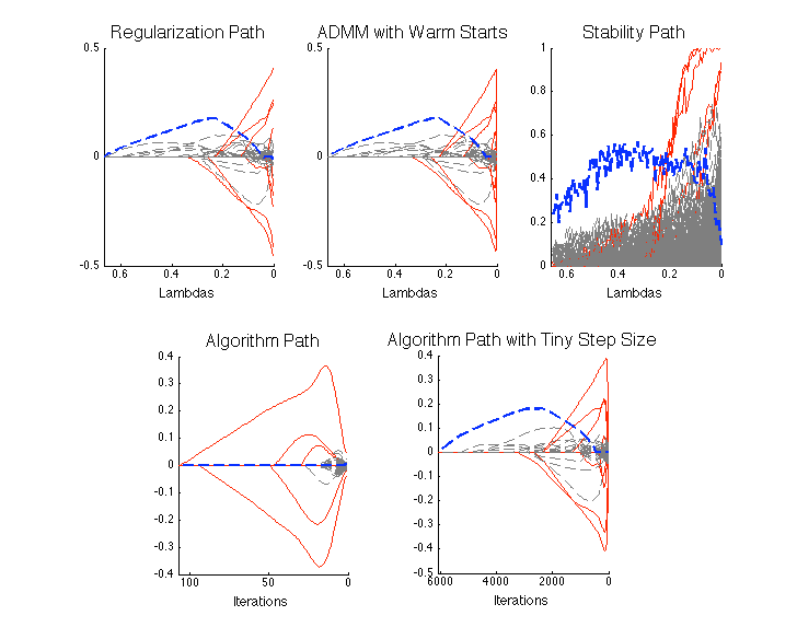
Figure 2: Comparisons of Algorithmic Regularization Paths (bottom panel) to regularization paths (top left and middle) and stability paths (top right) for the sparse linear regression example. The $--$ lines denote false variables, — lines denote true non-zero variables, and $--$ lines denote some highlighted false positives. Regularization paths were computed via the popular shooting method friedman2010regularization (top left) and our ADMM algorithm with warm-starts (top middle). Our Algorithmic Regularization Path with a tiny step size (bottom right) closely approximates the sparsity patterns of the regularization paths, while our method with a larger step size (bottom left) dramatically differs from the regularization paths. Notice that sparse regression in this example does a poor job of variable selection, selecting many false positives before any true features enter the model. Even the stability paths (top right) select many false positives. Our Algorithmic Regularization Path with a larger step-size, however, selects many of the true variables with much fewer false positives.

First, we verify empirically that that our ADMM algorithm with warm starts is equivalent to the regularization path (top left and top middle). Additionally, notice that, as expected, our Algorithm Path with a tiny step size (bottom right) also well approximates the sequence of active sets given by the regularization paths. With a larger step-size, however, our algorithm path (bottom left) yields a sequence of sparse models that differ markedly from the sparsity patterns of the regularization paths. This occurs as the change in regularization levels of each step are large enough so that the sparsity levels of the $\operatorname{\mathbf{z}}$-subproblem after the one-step approximation are not equivalent to that of the solution to (2).

Despite this, Figure 2 suggests that our Algorithm Paths with larger step sizes may have some advantages in terms of variable selection. Notice that regularization paths select many false positives (blue and gray dashed lines) before the true positives (red lines). This is expected as we used a real microarray data set for $\operatorname{\mathbf{X}}$ consisting of strongly correlated variables that directly violate the irrepresentable conditions under which variable selection for sparse regression is achievable buhlmann2011statistics . Our method, however, selects several true variables before the first false positive enters the model. To understand this further, we compare our approach to the Stability Paths used for stability selection meinshausen2010stability , a re-sampling scheme with some of the strongest theoretical guarantees for variable selection. The stability paths, however, also select several false positives. This as well as other empirical results that are omitted for space reasons suggest that our Algorithm Path with moderate or larger step sizes may perform better than convex optimization techniques in terms of variable selection. While a theoretical investigation of this is beyond the scope of this book chapter, the intuition for this is readily apparent. Our Algorithm Path starts from a dense solution and uses a ridge-like penalty. Thus, coefficients of highly correlated variables are likely to be grouped and have similar magnitude coefficient values. When soft-thresholding is performed in the $\operatorname{\mathbf{z}}$-subproblem, variables which are strongly correlated are likely to remain together in the model for at least the first several algorithm iterations. By keeping correlated variables together in the model longer and otherwise eliminating irrelevant variables, this gives our algorithm a better chance of selecting the truly non-zero variables out of a correlated set. Hence, the fact that we start with a dense solution seems to help us; this is in contrast to the LASSO, LAR and OMP paths which are initialized with an empty active set and greedily add variables most correlated with the response osborne2000new ; efron2004least . We plan on investigating our methods in terms of variable selection in future work.

Table 1: Timing comparison (averaged over 50 replications) of our ADMM Algorithmic Regularization Paths, Regularization Paths obtained from the shooting method (coordinate descent) & Stability Paths for different numbers of variables in the true model.

Time (seconds)	Algorithmic Regularization Path	Regularization Path	Stability Path
s = 20, p = 4000	0.0481	0.1322	36.6813
s = 20, p = 6000	0.0469	0.1621	43.9320

Finally, we compare our Algorithm Paths to state-of-the-art methods for computing the sparse regression regularization paths in terms of computational time in Table 1. The regularization paths were computed using the glmnet R package friedman2010regularization which is based on shooting (coordinate descent) routines friedman2010regularization . This approach and software is widely regarded as one of the fastest solvers for sparse regression. Notice that our Algorithm Paths, coded entirely in Matlab, run in about a fifth of the time as this state-of-the-art competitor. Also, our computational time is far superior to the re-sampling schemes required to compute the stability paths.

Overall, our Algorithmic Regularization Path for sparse linear regression reveals major computational advantages for finding a sequence of sparse models that approximate the active sets of regularization paths. Additionally, empirical evidence suggests that our methods may also enjoy some important statistical advantages in terms of variable selection that we will explore in future work.

3.2 Reduced-Rank Multi-Task Learning

Our ADMM Algorithmic Regularization Path applies generally to many convex penalty types beyond the $\ell_{1}$-norm. Here, we demonstrate our method in conjunction with a reduced-rank multi-task learning problem also called multi-response regression. This problem has been studied by negahban2011estimation among many others.

Suppose we observe $n$ iid samples measured on $p$ covariates and for $q$ outcomes, yielding a covariate matrix, $\operatorname{\mathbf{X}}\in\Re^{n\times p}$, and a response matrix $\operatorname{\mathbf{Y}}\in\Re^{n\times q}$. Then, our goal is to fit the following statistical model: $\operatorname{\mathbf{Y}}=\operatorname{\mathbf{X}}\operatorname{\mathbf{B}}+\mathbf{\epsilon}$, where $\operatorname{\mathbf{B}}$ is the $p\times q$ coefficient matrix which we seek to learn, and $\mathbf{\epsilon}$ is independent noise. As often the number of covariates is large relative to the sample size, $pq\gg n$, many have suggested to regularize the coefficient matrix $\operatorname{\mathbf{B}}$ by assuming it has a low-rank structure, $\mathrm{rank}(\operatorname{\mathbf{B}})<p\wedge q$. Thus, our model space of sparse solutions is given by the space of all possible reduced-rank solutions. Exploring this space is an NP hard computational problem; thus, many have employed the nuclear norm penalty, $\lVert\operatorname{\mathbf{B}}\rVert_{*}=\sum_{j=1}^{p\wedge q}\sigma_{j}(\operatorname{\mathbf{B}})$, which is the sum (or $\ell_{1}$-norm) of the singular values of $\operatorname{\mathbf{B}}$, $\sigma(\operatorname{\mathbf{B}})$, and the tightest convex relaxation of the rank constraint. Thus, we arrive at the following optimization problem:

$$\underset{\operatorname{\mathbf{B}}}{\text{minimize}}\quad\frac{1}{2}\lVert\operatorname{\mathbf{Y}}-\operatorname{\mathbf{X}}\operatorname{\mathbf{B}}\rVert_{\text{F}}^{2}+\lambda\lVert\operatorname{\mathbf{B}}\rVert_{*}$$ (4)

Here, $\lVert\cdot\rVert_{\text{F}}$ is the Frobenious norm, $\lambda\geq 0$ is the regularization parameter controlling the rank of the solution and $\lVert\cdot\rVert_{*}$ is the nuclear norm penalty.

For model selection then, one seeks to explore the sequence of low-rank solutions obtained as $\lambda$ varies. To develop our Algorithm Path for approximating this sequence of low-rank solutions, let us consider the ADMM sub-problems for solving (4). The augmented Lagrangian, sub-problems, dual updates are analogous to that of the sparse linear regression example, and hence we omit these here. Examining the $\operatorname{\mathbf{Z}}$-subproblem, however, recall that this is the proximal operator for the nuclear norm penalty: $\operatorname{\mathbf{Z}}^{k}=\underset{\operatorname{\mathbf{Z}}}{\arg\min}\;\frac{1}{2}\lVert\operatorname{\mathbf{Z}}-(\operatorname{\mathbf{B}}^{k}+\operatorname{\mathbf{U}}^{k})\rVert_{\text{F}}^{2}+\gamma\lVert\operatorname{\mathbf{Z}}\rVert_{*}$, which can be solved by soft-thresholding the singular values: Suppose that $\mathbf{A}=\operatorname{\mathbf{U}}\bm{\Sigma}\mathbf{V}^{\sf T}$ is the SVD of $\mathbf{A}$. Then singular-value thresholding is defined as $\text{SVT}_{\gamma}(\mathbf{A})=\operatorname{\mathbf{U}}[\mathrm{diag}((\bm{\sigma}-\gamma)_{+})]\mathbf{V}^{\sf T}$ and the solution for the $\operatorname{\mathbf{Z}}$ sub-problem is $\operatorname{\mathbf{Z}}^{k}=\text{SVT}_{\gamma}(\operatorname{\mathbf{B}}^{k}+\operatorname{\mathbf{U}}^{k})$.

Algorithm 4 Algorithmic Regularization Path for Reduced-Rank Regression

1. Initialize: $\operatorname{\mathbf{Z}}^{0}=\mathbf{0}$, $\operatorname{\mathbf{U}}^{0}=\mathbf{0}$, $\gamma^{0}=\epsilon$, and step size $t>0$.

2. Precompute: $\operatorname{\mathbf{H}}=(\operatorname{\mathbf{X}}^{\sf T}\operatorname{\mathbf{X}}/n+\operatorname{\mathbf{I}})^{-1}$ and $\operatorname{\mathbf{H}}\operatorname{\mathbf{X}}^{\sf T}\operatorname{\mathbf{Y}}$.

3. While $\lVert\operatorname{\mathbf{Z}}^{k}\rVert\neq 0$
         $\gamma^{k}=\gamma^{k-1}+t$ (or $\gamma^{k}=\gamma^{k-1}t$).
         $\operatorname{\mathbf{B}}^{k}=\operatorname{\mathbf{H}}\operatorname{\mathbf{X}}^{\sf T}\operatorname{\mathbf{Y}}+\operatorname{\mathbf{H}}(\operatorname{\mathbf{Z}}^{k-1}-\operatorname{\mathbf{U}}^{k-1})$.
         $\operatorname{\mathbf{Z}}^{k}=\text{SVT}_{\gamma^{k}}(\operatorname{\mathbf{B}}^{k}+\operatorname{\mathbf{U}}^{k-1})$.     (Record $\operatorname{\mathbf{Z}}^{k}$ at each iteration.)
         $\operatorname{\mathbf{U}}^{k}=\operatorname{\mathbf{U}}^{k-1}+\operatorname{\mathbf{B}}^{k}-\operatorname{\mathbf{U}}^{k}$
   end

4. Output $\{\operatorname{\mathbf{Z}}^{k}:k=1,\cdots,K\}$ as the algorithmic regularization path.

Then, following the framework of the sparse linear regression example, our ADMM Algorithmic Regularization Path for the reduced-rank mutli-task learning (regression) is outlined in Algorithm 4. Notice that the algorithm has the same basic steps as in the previous example except that solving the proximal operator for the $\operatorname{\mathbf{Z}}$ sub-problem entails singular value thresholding. This step is the most computationally time consuming aspect of the algorithm as $K$ total SVDs must be computed to approximate the sequence of solutions. Also note that similarly to the sparse regression example, the inversion needed, $(\operatorname{\mathbf{X}}^{\sf T}\operatorname{\mathbf{X}}/n+\operatorname{\mathbf{I}})^{-1}$, can be precomputed by using the matrix inversion identities as previously discussed and cached as a convenient factorization; hence, this is computationally feasible even when $p\gg n$.

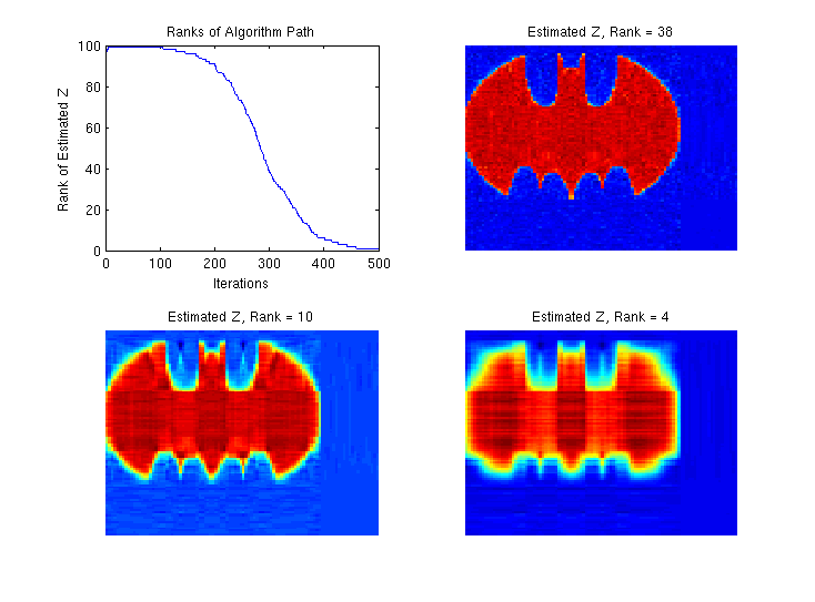
Figure 3: Reduced Rank Regression simulated example. The true coefficient matrix, $\operatorname{\mathbf{B}}\in\Re^{100\times 100}$, is an image of batman that is rank 38. Our Algorithm Path provides a sequence of low-ranks solutions at a fine resolution (top left) that well-approximate the low-rank signal; three such low-rank solutions (top right and bottom panel) are shown from iterates of our Algorithm Path.

	# Ranks Considered	# SVDs	Time in Seconds
Algorithm Path	90	476	2.354
Proximal Gradient	57	2519	12.424
ADMM	51	115,946	599.144

Table 2: Algorithm comparisons for reduced rank regression example.

To demonstrate the computational advantages of our approach, we conduct a small simulation study comparing our method to the two most commonly used algorithms for reduced-rank regression: proximal gradient descent and ADMM. First, we generate data according to the model: $\operatorname{\mathbf{Y}}=\operatorname{\mathbf{X}}\operatorname{\mathbf{B}}+\mathbf{\epsilon}$, where $\operatorname{\mathbf{X}}_{200\times 100}$ is generated as independent standard Gaussians, $\operatorname{\mathbf{B}}_{100\times 100}$ is an image of the Batman symbol, and $\mathbf{\epsilon}_{200\times 100}$ is independent standard Gaussian noise. We set the signal in the coefficient matrix to be a low-rank image of the Batman symbol, $\mathrm{rank}(\operatorname{\mathbf{B}})=38$, which can be well-approximated by further reduced rank images. We applied our Algorithmic Regularization Paths to this simulated example with 500 logarithmically-spaced values of $\gamma$. Results are given in Figure 3 and show that our Algorithm Path smoothly explores the model space of reduced rank solutions and nicely approximates the true signal as a low-rank batman image. We also conduct a timing comparison to implementations of proximal gradient descent and ADMM algorithms using warm-starts for this same example; results are given in Table 2. Here, we see that our approach requires much fewer SVD computations and is much faster than both algorithms, especially the ADMM algorithm. Additionally, both the ADMM and proximal gradient algorithm employed 100 logarithmically spaced values of the regularization parameter, $\lambda$. With this, however, we see that not all possible ranks of the model space are considered, with proximal gradient and ADMM considering 57 and 51 ranks out of 100 respectively. In contrast, our Algorithmic Regularization Path yields a sequence of sparse solutions at a much finer resolution, considering 90 out of the 100 possible ranks. Thus, for proximal gradient and ADMM algorithms to consider the same range of possible sparsity levels (ranks), a greater number of problems would have to be solved over a much finer grid of regularization parameters, further inflating compute times.

Overall, our approach yields substantial computational savings for computing a sequence of sparse solutions for reduced rank regression compared to other state-of-the-art methods for this problem.

3.3 Convex Clustering

Our final example applies the ADMM Algorithmic Regularization path to an example with fusion type or non-separable penalties, namely a recently introduced convex formulation of cluster analysis ChiLan2013 ; HocVerBac2011 ; LinOhlLju2011 . Given $n$ points ${\bm{\mathbf{{y}}}}_{1},\ldots,{\bm{\mathbf{{y}}}}_{n}$ in $\Re^{p}$, we pose the clustering problem as follows. Assign to each point ${\bm{\mathbf{{y}}}}_{i}$ its own cluster center ${\bm{\mathbf{{\bm{\beta}}}}}_{i}\in\Re^{p}$. We then seek an assignment of ${\bm{\mathbf{{\bm{\beta}}}}}_{i}$ that minimizes the distances between ${\bm{\mathbf{{y}}}}_{i}$ and ${\bm{\mathbf{{\bm{\beta}}}}}_{i}$ and seeks sparsity between cluster center pairs ${\bm{\mathbf{{\bm{\beta}}}}}_{i}$ and ${\bm{\mathbf{{\bm{\beta}}}}}_{j}$. Computing all possible cluster assignments, however, is an NP hard problem. Hence, the following relaxation poses finding the cluster assignments as a convex optimization problem:

$$\underset{{\bm{\mathbf{{\bm{\beta}}}}}_{1},\ldots,{\bm{\mathbf{{\bm{\beta}}}}}_{n}}{\text{minimize}}\;\frac{1}{2}\sum_{i=1}^{n}\lVert{\bm{\mathbf{{y}}}}_{i}-{\bm{\mathbf{{\bm{\beta}}}}}_{i}\rVert_{2}^{2}+\lambda\sum_{i<j}w_{ij}\lVert{\bm{\mathbf{{\bm{\beta}}}}}_{i}-{\bm{\mathbf{{\bm{\beta}}}}}_{j}\rVert_{2},$$ (5)

where $\lambda$ is a positive regularization parameter, and $w_{ij}$ is a nonnegative weight. When $\lambda=0$, the minimum is attained when ${\bm{\mathbf{{\bm{\beta}}}}}_{i}={\bm{\mathbf{{y}}}}_{i}$, and each point occupies a unique cluster. As $\lambda$ increases, the cluster centers begin to coalesce. Two points ${\bm{\mathbf{{y}}}}_{i}$ and ${\bm{\mathbf{{y}}}}_{j}$ with ${\bm{\mathbf{{\bm{\beta}}}}}_{i}={\bm{\mathbf{{\bm{\beta}}}}}_{j}$ are said to belong to the same cluster. For sufficiently large $\lambda$ all points coalesce into a single cluster at $\overline{{\bm{\mathbf{{y}}}}}$, the mean of the ${\bm{\mathbf{{y}}}}_{i}$. Because the objective in (5) is strictly convex and coercive, it possesses a unique minimizer for each value of $\lambda$. This is in stark contrast to other typical criteria used for clustering, which often rely on greedy algorithms that are prone to get trapped in suboptimal local minima. Because of its coalescent behavior, the resulting solution path can be considered a convex relaxation of hierarchical clustering HocVerBac2011 .

This problem generalizes the fused LASSO TibSauRos2005 , and as with other fused LASSO problems, penalizing affine transformations of the decision variable makes minimization challenging in general. The one exception is when a 1-norm is used instead of the 2-norm in the fusion penalty terms. In this case, the problem reduces to a weighted one-dimensional total variation denoising problem. Under other norms, including the 2-norm, the situation, is salvageable if we adopt a splitting strategy discussed earlier in Section 1.1 for dealing with fusion type or non-separable penalties. Briefly, we consider using the 2-norm in the fusion penalty to be most broadly applicable since the solutions to the convex clustering problem become invariant to rotations in the data. Consequently, clustering assignments will also be guaranteed to be rotationally invariant.

Let the variables ${\bm{\mathbf{{z}}}}_{ij}\in\Re^{p}$ record the differences between the $i$th and $j$th points. We denote the collections of variables $\{{\bm{\mathbf{{\bm{\beta}}}}}_{i}\}_{i=1}^{n}$ and $\{{\bm{\mathbf{{\bm{z}}}}}_{ij}\}_{i<j}$ by ${\bm{\mathbf{{\bm{\beta}}}}}$ and ${\bm{\mathbf{{z}}}}$ respectively. Then the original problem can be reformulated as:

$$\begin{split}\underset{{\bm{\mathbf{{\bm{\beta}}}}},{\bm{\mathbf{{z}}}}}{\text{minimize}}\;\;\frac{1}{2}\sum_{i=1}^{n}\lVert{\bm{\mathbf{{y}}}}_{i}-{\bm{\mathbf{{\bm{\beta}}}}}_{i}\rVert_{2}^{2}+\lambda\sum_{i<j}w_{ij}\lVert{\bm{\mathbf{{z}}}}_{ij}\rVert_{2}\quad\text{subject to}\quad{\bm{\mathbf{{\bm{\beta}}}}}_{i}-{\bm{\mathbf{{\bm{\beta}}}}}_{j}-{\bm{\mathbf{{z}}}}_{ij}={\bm{\mathbf{{0}}}}.\end{split}$$ (6)

Consider the ADMM algorithm derived in ChiLan2013 for solving (6). Let ${\bm{\mathbf{{u}}}}_{ij}\in\Re^{p}$ denote the Lagrange multiplier for the $ij$th equality constraint. Let ${\bm{\mathbf{{u}}}}$ denote the collection of variables $\{{\bm{\mathbf{{u}}}}_{ij}\}_{i<j}$. The augmented Lagrangian is given by:

$$\mathcal{L}({\bm{\mathbf{{\bm{\beta}}}}},{\bm{\mathbf{{z}}}},{\bm{\mathbf{{u}}}})=\frac{1}{2}\sum_{i=1}^{n}\lVert{\bm{\mathbf{{y}}}}_{i}-{\bm{\mathbf{{\bm{\beta}}}}}_{i}\rVert_{2}^{2}+\lambda\sum_{i<j}{w}_{ij}\lVert{\bm{\mathbf{{z}}}}_{ij}\rVert_{2}+\frac{1}{2}\sum_{i<j}\lVert{\bm{\mathbf{{\bm{\beta}}}}}_{i}-{\bm{\mathbf{{\bm{\beta}}}}}_{j}-{\bm{\mathbf{{z}}}}_{ij}+{\bm{\mathbf{{u}}}}_{ij}\rVert_{2}^{2}.$$

Then, the three ADMM subproblems are given by:

$${\bm{\mathbf{{\bm{\beta}}}}}^{k+1} = \underset{{\bm{\mathbf{{\bm{\beta}}}}}}{\arg\min}\;\frac{1}{2}\sum_{i=1}^{n}\lVert{\bm{\mathbf{{y}}}}_{i}-{\bm{\mathbf{{\bm{\beta}}}}}_{i}\rVert_{2}^{2}+\frac{1}{2}\sum_{i<j}\lVert{\bm{\mathbf{{\bm{\beta}}}}}_{i}-{\bm{\mathbf{{\bm{\beta}}}}}_{j}-{\bm{\mathbf{{z}}}}_{ij}+{\bm{\mathbf{{u}}}}_{ij}\rVert_{2}^{2}$$

$${\bm{\mathbf{{z}}}}^{k+1} = \underset{{\bm{\mathbf{{z}}}}}{\arg\min}\;\lambda\sum_{i<j}{w}_{ij}\lVert{\bm{\mathbf{{z}}}}_{ij}\rVert_{2}+\frac{1}{2}\sum_{i<j}\lVert{\bm{\mathbf{{\bm{\beta}}}}}_{i}-{\bm{\mathbf{{\bm{\beta}}}}}_{j}-{\bm{\mathbf{{z}}}}_{ij}+{\bm{\mathbf{{u}}}}_{ij}\rVert_{2}^{2}$$

$${\bm{\mathbf{{u}}}}^{k+1}_{ij} = {\bm{\mathbf{{u}}}}^{k}_{ij}+[{\bm{\mathbf{{z}}}}^{k+1}_{ij}-({\bm{\mathbf{{\bm{\beta}}}}}^{k+1}_{i}-{\bm{\mathbf{{\bm{\beta}}}}}^{k+1}_{j})].$$

Splitting the variables in this manner allows us to solve a series of straightforward subproblems. Updating ${\bm{\mathbf{{\bm{\beta}}}}}$ involves solving a ridge regression problem. Despite the fact that the quadratic penalty term is not separable in the ${\bm{\mathbf{{\bm{\beta}}}}}$, after some algebraic maneuvering, which is detailed in ChiLan2013 , it is possible to explicitly write down the updates for each ${\bm{\mathbf{{\bm{\beta}}}}}$ separately:

$${\bm{\mathbf{{\bm{\beta}}}}}^{k+1}_{i} = \left[\frac{1}{1+n}{\bm{\mathbf{{y}}}}_{i}+\frac{n}{1+n}\overline{{\bm{\mathbf{{y}}}}}\right]+\frac{1}{1+n}\left[\sum_{j>i}[{\bm{\mathbf{{u}}}}^{k}_{ij}+{\bm{\mathbf{{z}}}}^{k}_{ij}]-\sum_{j<i}[{\bm{\mathbf{{u}}}}^{k}_{ji}+{\bm{\mathbf{{z}}}}^{k}_{ji}]\right].$$

Updating ${\bm{\mathbf{{z}}}}$ requires minimizing an objective that separates in each of the ${\bm{\mathbf{{z}}}}_{ij}$,

$${\bm{\mathbf{{z}}}}^{k+1}_{ij} = \underset{{\bm{\mathbf{{z}}}}_{ij}}{\arg\min}\;\frac{1}{2}\lVert{\bm{\mathbf{{z}}}}_{ij}-[{\bm{\mathbf{{\bm{\beta}}}}}^{k+1}_{i}-{\bm{\mathbf{{\bm{\beta}}}}}^{k+1}_{j}-{\bm{\mathbf{{u}}}}^{k}_{ij}]\rVert_{2}^{2}+\lambda{w}_{ij}\lVert{\bm{\mathbf{{z}}}}_{ij}\rVert_{2}.$$

This step can be computed explicitly using the block-wise soft-thresholding operator, the proximal operator of the group LASSO YuaLin2006 , namely,

$$S({\bm{\mathbf{{z}}}},\tau)=\underset{{\bm{\mathbf{{\zeta}}}}}{\arg\min}\;\frac{1}{2}\lVert{\bm{\mathbf{{\zeta}}}}-{\bm{\mathbf{{z}}}}\rVert_{2}^{2}+\tau\lVert{\bm{\mathbf{{\zeta}}}}\rVert_{2}=\left[1-\frac{\tau}{\lVert{\bm{\mathbf{{z}}}}\rVert_{2}}\right]_{+}{\bm{\mathbf{{z}}}},$$

where $a_{+}=\max(a,0)$ and $\tau\geq 0$ controls the amount of shrinkage towards zero.

For model selection purposes, one typically studies the sequence of cluster assignments given by coalescent patterns of $\operatorname{\bm{\beta}}$, or the sparse patterns in the first differences of $\operatorname{\bm{\beta}}$, as $\lambda$ varies. We then seek to quickly approximate this sequence of active sets given by the coalescent patterns of $\operatorname{\bm{\beta}}$ with our Algorithmic Regularization Paths, summarized in Algorithm 5.

Algorithm 5 Algorithmic Regularization Path for Convex Clustering

1. Initialize ${\bm{\mathbf{{z}}}}^{0}_{ij}={\bm{\mathbf{{0}}}}$, ${\bm{\mathbf{{u}}}}^{0}_{ij}={\bm{\mathbf{{0}}}}$, $\gamma^{(0)}=\varepsilon$, $k=1$, and set $t>0$.

2. While $\lVert{\bm{\mathbf{{z}}}}^{k}\rVert_{\text{F}}>0$:

   for all $i$ do

        ${\bm{\mathbf{{\bm{\beta}}}}}^{k+1}_{i}=\left[\frac{1}{1+n}{\bm{\mathbf{{y}}}}_{i}+\frac{n}{1+n}\overline{{\bm{\mathbf{{y}}}}}\right]+\frac{1}{1+n}\left[\sum_{j>i}[{\bm{\mathbf{{u}}}}^{k}_{ij}+{\bm{\mathbf{{z}}}}^{k}_{ij}]-\sum_{j<i}[{\bm{\mathbf{{u}}}}^{k}_{ji}+{\bm{\mathbf{{z}}}}^{k}_{ji}]\right]$

   end for

   for all $i<j$ do

        ${\bm{\mathbf{{z}}}}^{k+1}_{ij}=S\left({\bm{\mathbf{{\bm{\beta}}}}}^{k+1}_{i}-{\bm{\mathbf{{\bm{\beta}}}}}^{k+1}_{j}-{\bm{\mathbf{{u}}}}^{k}_{ij},\gamma^{(k)}{w}_{ij}\right)$

        ${\bm{\mathbf{{u}}}}^{k+1}_{ij}={\bm{\mathbf{{u}}}}^{k}_{ij}+[{\bm{\mathbf{{z}}}}^{k+1}_{ij}-({\bm{\mathbf{{\bm{\beta}}}}}^{k+1}_{i}-{\bm{\mathbf{{\bm{\beta}}}}}^{k+1}_{j})],$

   end for

   $\gamma^{(k+1)}=t\gamma^{(k)}$

3. Output $\left\{{\bm{\mathbf{{z}}}}^{k}_{ij}\right\}$ as the algorithm path .

As in the general case, we can use iterates of the $\operatorname{\mathbf{z}}$-subproblem to approximate a sparse sequence of cluster assignments. Given ${\bm{\mathbf{{z}}}}$, we can determine a clustering assignment in time that is linear in the number of data points $n$. We simply apply breadth-first search to identify the connected components of the following graph induced by the ${\bm{\mathbf{{z}}}}$. The graph identifies a node with every data point and places an edge between the $i$th and $j$th node if and only if ${\bm{\mathbf{{z}}}}_{ij}={\bm{\mathbf{{0}}}}$. Each connected component corresponds to a cluster.

We now illustrate on a simulated “halfmoon” data set of $n=200$ points in $\Re^{2}$, that computing our Algorithm Path can lead to non-trivial computational cost savings for obtaining a sequence of clustering assingments. We first detail some preliminaries. Although we do not take the space to discuss it here, in practice the choice of weights is very important. This topic is explored in ChiLan2013 , and we use the sparse kernel weights which were shown to work well empirically in that paper. We created a geometric sequence of parameters $\lambda^{(k)}$ and $\gamma^{(k)}$, namely given a fixed multiplicative factor $t>1$, we set $\lambda^{(k+1)}=t\lambda^{(k)}$. The sequence $\gamma^{(k)}$ was constructed similarly, although we study our Algorithm Paths for several multiplicative factors, $t\in\{1.1,1.05,1.01\}$.

In contrast to the regularization path, the Algorithm Path does not require any convergence checks since only one step is taken at each grid point. Nonetheless, we only report the number of rounds of ADMM updates taken by each approach. The Algorithm Path took $259,1294,$ and $2,536$ rounds of updates for the three step sizes considered; in contrast, the regularization path even for a very modest tolerance level, $10^{-4}$, required a grand total of 30,008 rounds of updates, substantially more than our approach.

Figure 4 shows the ADMM Algorithmic Regularization paths and regularization path respectively for this simulated example. For each data point $i$ we plot the sequence of the segments between consecutive estimates of its center, namely $\bm{\beta}_{i}^{k+1}$ and $\bm{\beta}_{i}^{k}$. These paths begin to overlap and merge into “trunks” when center estimates for close-by data points begin to coincide as the parameters $\lambda^{(k)}$ and $\gamma^{(k)}$ becomes sufficiently large. For sufficiently small step sizes for the regularization levels the Algorithm Path and regularization path are strikingly similar, as expected and demonstrated previously in our other examples. For larger step sizes, however, the paths differ markedly, but still appear to capture the same clustering assignments. Overall, although the simulated data is relatively small, computing the whole regularization path, even for a modest stopping tolerance can, requires an order of magnitude more iterations and computational time than the Algorithm Path.

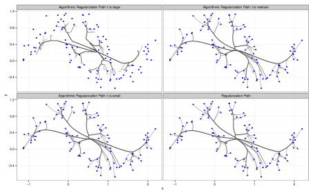
Figure 4: Convex clustering on simulated data: In the first three panels (from left to right, top to bottom), lines trace the ADMM Algorithmic Regularization path of the individual cluster centers as the algorithm path parameter $\gamma$ increases for $t=1.1$ (large), $1.05$ (medium), and $1.01$ (small). In the panel in the lower right corner, the lines trace the regularization path of the individual cluster centers as the regularization parameter $\lambda$ increases.

4 Discussion

In this chapter, we have presented a novel framework for approximating the sequence of active sets associated with regularization paths of sparse statistical learning problems. Instead of solving optimization problems over a grid of penalty parameters as in traditional regularization paths, our algorithm performs a series of one-step approximations to an ADMM algorithm employing warm-starts with the goal of estimating a good sequence of sparse models. Our approach has a number of advantages including easy implementation, exploration of the sparse model space at a fine resolution, and most importantly fast compute times; we have demonstrated these advantages through several sparse statistical learning examples.

In our demonstrations, we have focused simply on computing the full sequence of active sets corresponding to the regularization path which is the critical computationally intensive step in the process of model selection. Once the sequence of sparse models has been found, common methods for model selection such as AIC, BIC, cross-validation and stability selection, can be employed to choose the optimal model. We note that with regularization paths, model selection procedures typically choose the optimal $\lambda$ which indexes the optimal sparse model. For our Algorithm Paths which do not directly solve regularized statistical problems, model selection procedures should be used to choose the optimal iteration, $k$, and the corresponding sparse model given by the active set of $\operatorname{\mathbf{z}}^{k}$. While this chapter has focused on finding the sequence of sparse models via our Algorithm Paths, we plan to study using these paths in conjunction with common model selection procedures in future work.

As the ADMM algorithm has been widely used for sparse statistical learning problems, the mechanics are in place for broad application of our Algorithm Paths which utilize the three standard ADMM subproblems. Indeed, our approach could potentially yield substantial computational savings for any ADMM application where the $\operatorname{\bm{\beta}}$ and $\operatorname{\mathbf{z}}$ can be solved efficiently. Furthermore, there has been much recent interest in distributed versions of ADMM algorithms yin2013parallel ; mota2012distributed . Thus, there is the potential to use these in conjunction with our problem to distribute computation in the $\operatorname{\bm{\beta}}$ and $\operatorname{\mathbf{z}}$ subproblems and further speed computations for Big-Data problems. Also, we have focused on developing our Algorithm Path for sparse statistical learning problems that can be written as a composite of a smooth loss function and a non-smooth, convex penalty. Our methods, however, can be easily extended to study constrained statistical learning problems, such as that of the support vector machines. Finally, our framework utilizes the ADMM splitting method, but the strategies we develop could also be useful for computing a sequence of sparse models using other operator splitting algorithms.

Our work raises many questions from statistical and optimization perspectives. Further work needs to be done to characterize and study the mathematical properties of the Algorithm Paths as well as relate them to existing optimization procedures and algorithms. For example, ADMM is just one of many variants of proximal methods parikh2013proximal . We suspect that other variants, such as proximal gradient descent, used to fit sparse models will also benefit from an Algorithm Path approach in expediting the model selection procedure. We leave this as future work.

In our demonstrations in Section 3, we suggested empirically that our Algorithm Paths with a tiny step size closely approximate the sequence of active sets associated with regularization paths. Further work needs to be done to verify this connection mathematically. Along these lines, a key practical question is how to choose the appropriate step size for increasing the amount of regularization as the algorithm progresses. As we have demonstrated, changing the step size yields paths with very different solutions and behaviors that warrant further investigation. For now, our recommendation is to employ a fairly small step size as these well-approximate the traditional regularization paths in all of the examples we have studied. Additionally, our approach may be related to other new proposals for computing regularization paths based on partial differential equations, for example shinew ; these potential connections merit further investigation.

Our work also raises a host of interesting statistical questions as well. The sparse regression example suggested that Algorithm Paths may not simply yield computational savings, but may also perform better in terms of variable selection. This raises an interesting statistical prospect that we plan to carefully study in future work.

To conclude, we have introduced a novel approach to approximating the sequence of active sets associated with regularization paths for large-scale sparse statistical learning procedures. Our methods yield substantial computational savings and raise a number of interesting open questions for future research.

References

- (1) Aguiar, P., Xing, E.P., Figueiredo, M., Smith, N.A., Martins, A.: An augmented Lagrangian approach to constrained MAP inference. In: Proceedings of the 28th International Conference on Machine Learning (ICML-11), pp. 169–176 (2011)
- (2) Bien, J., Taylor, J., Tibshirani, R.: A lasso for hierarchical interactions. The Annals of Statistics 41(3), 1111–1141 (2013)
- (3) Boyd, S., Parikh, N., Chu, E., Peleato, B., Eckstein, J.: Distributed optimization and statistical learning via the alternating direction method of multipliers. Foundations and Trends® in Machine Learning 3(1), 1–122 (2011)
- (4) Bühlmann, P., Van De Geer, S.: Statistics for high-dimensional data: methods, theory and applications. Springer (2011)
- (5) Chi, E.C., Lange, K.: Splitting methods for convex clustering. Journal of Computational and Graphical Statistics In press
- (6) Danaher, P., Wang, P., Witten, D.M.: The joint graphical lasso for inverse covariance estimation across multiple classes. Journal of the Royal Statistical Society: Series B (Statistical Methodology) 76(2), 373–397 (2014)
- (7) Donoho, D.L., Tsaig, Y., Drori, I., Starck, J.L.: Sparse solution of underdetermined systems of linear equations by stagewise orthogonal matching pursuit. Information Theory, IEEE Transactions on 58(2), 1094–1121 (2012)
- (8) Efron, B., Hastie, T., Johnstone, I., Tibshirani, R., et al.: Least angle regression. The Annals of statistics 32(2), 407–499 (2004)
- (9) Friedman, J., Hastie, T., Höfling, H., Tibshirani, R., et al.: Pathwise coordinate optimization. The Annals of Applied Statistics 1(2), 302–332 (2007)
- (10) Friedman, J., Hastie, T., Tibshirani, R.: Regularization paths for generalized linear models via coordinate descent. Journal of statistical software 33(1), 1 (2010)
- (11) Goldstein, T., ODonoghue, B., Setzer, S.: Fast alternating direction optimization methods. CAM report pp. 12–35 (2012)
- (12) Goldstein, T., Osher, S.: The split Bregman method for L1-regularized problems. SIAM J. Img. Sci. 2(2), 323–343 (2009)
- (13) Hager, W.W.: Updating the inverse of a matrix. SIAM review 31(2), 221–239 (1989)
- (14) Hastie, T., Rosset, S., Tibshirani, R., Zhu, J.: The entire regularization path for the support vector machine. Journal of Machine Learning Research 5, 1391–1415 (2004)
- (15) Hastie, T., Tibshirani, R., Friedman, J., Hastie, T., Friedman, J., Tibshirani, R.: The elements of statistical learning, 2 edn. 1. Springer (2009)
- (16) He, B., Yang, H., Wang, S.: Alternating direction method with self-adaptive penalty parameters for monotone variational inequalities. Journal of Optimization Theory and applications 106(2), 337–356 (2000)
- (17) Hocking, T., Vert, J.P., Bach, F., Joulin, A.: Clusterpath: an algorithm for clustering using convex fusion penalties. In: L. Getoor, T. Scheffer (eds.) Proceedings of the 28th International Conference on Machine Learning (ICML-11), ICML ’11, pp. 745–752 (2011)
- (18) Hu, Y., Allen, G.I.: Local-aggregate modeling for big-data via distributed optimization: Applications to neuroimaging. arXiv preprint arXiv:1405.0629 (2014)
- (19) Lindsten, F., Ohlsson, H., Ljung, L.: Just relax and come clustering! A convexification of -means clustering. Tech. rep., Linköpings universitet (2011)
- (20) Liu, J., Musialski, P., Wonka, P., Ye, J.: Tensor completion for estimating missing values in visual data. In: Computer Vision, 2009 IEEE 12th International Conference on, pp. 2114–2121. IEEE (2009)
- (21) Ma, S., Xue, L., Zou, H.: Alternating direction methods for latent variable Gaussian graphical model selection. Neural Computation 25(8), 2172–2198 (2013)
- (22) Mairal, J., Jenatton, R., Obozinski, G., Bach, F.: Convex and network flow optimization for structured sparsity. The Journal of Machine Learning Research 12, 2681–2720 (2011)
- (23) Meinshausen, N., Bühlmann, P.: Stability selection. Journal of the Royal Statistical Society: Series B (Statistical Methodology) 72(4), 417–473 (2010)
- (24) Mohan, K., Chung, M., Han, S., Witten, D., Lee, S.I., Fazel, M.: Structured learning of Gaussian graphical models. In: Advances in Neural Information Processing Systems, pp. 629–637 (2012)
- (25) Mohan, K., London, P., Fazel, M., Witten, D., Lee, S.I.: Node-based learning of multiple Gaussian graphical models. Journal of Machine Learning Research 15, 445–488 (2014)
- (26) Mota, J.F., Xavier, J., Aguiar, P.M., Puschel, M.: Distributed basis pursuit. Signal Processing, IEEE Transactions on 60(4), 1942–1956 (2012)
- (27) Negahban, S., Wainwright, M.J., et al.: Estimation of (near) low-rank matrices with noise and high-dimensional scaling. The Annals of Statistics 39(2), 1069–1097 (2011)
- (28) Osborne, M.R., Presnell, B., Turlach, B.A.: A new approach to variable selection in least squares problems. IMA journal of numerical analysis 20(3), 389–403 (2000)
- (29) Parikh, N., Boyd, S.: Proximal algorithms. Foundations and Trends in optimization 1(3), 123–231 (2013)
- (30) Rosset, S., Ji, Z.: Piecewise linear regularized solution paths. The Annals of Statistics 35(3), 1012–1030 (2007)
- (31) Rudin, L.I., Osher, S., Fatemi, E.: Nonlinear total variation based noise removal algorithms. Physica D: Nonlinear Phenomena 60(1â4), 259–268 (1992)
- (32) Shi, J., Yin, W., Osher, S.: A new regularization path for logistic regression via linearized Bregman. Tech. rep., Rice CAAM Tech Report TR12-24 (2012)
- (33) Tibshirani, R.: Regression shrinkage and selection via the lasso. Journal of the Royal Statistical Society. Series B (Methodological) 58(1), 267–288 (1996)
- (34) Tibshirani, R., Saunders, M., Rosset, S., Zhu, J., Knight, K.: Sparsity and smoothness via the fused lasso. Journal of the Royal Statistical Society: Series B (Statistical Methodology) 67(1), 91–108 (2005)
- (35) Vu, V.Q., Cho, J., Lei, J., Rohe, K.: Fantope projection and selection: A near-optimal convex relaxation of sparse PCA. In: Advances in Neural Information Processing Systems 26, pp. 2670–2678 (2013)
- (36) Wahlberg, B., Boyd, S., Annergren, M., Wang, Y.: An ADMM algorithm for a class of total variation regularized estimation problems. arXiv preprint arXiv:1203.1828 (2012)
- (37) Wu, T.T., Lange, K., et al.: Coordinate descent algorithms for lasso penalized regression. The Annals of Applied Statistics 2(1), 224–244 (2008)
- (38) Yan, M., Yin, W.: Self equivalence of the alternating direction method of multipliers. arXiv preprint arXiv:1407.7400 (2014)
- (39) Yin, Z., Ming, P., Wotao, Y.: Parallel and distributed sparse optimization. Tech. rep., Rice University CAAM (2013)
- (40) Yuan, L., Liu, J., Ye, J.: Efficient methods for overlapping group lasso. In: NIPS, vol. 35, pp. 352–360 (2011)
- (41) Yuan, M., Lin, Y.: Model selection and estimation in regression with grouped variables. Journal of the Royal Statistical Society: Series B (Statistical Methodology) 68(1), 49–67 (2006)
- (42) Yuan, X., Yang, J.: Sparse and low-rank matrix decomposition via alternating direction method. The Pacific Journal of Optimization 9(1), 167–180 (2012)