Active Region Emergence & Remote Flares

Abstract

We study the effect of new emerging solar active regions on the large-scale magnetic environment of existing regions. We first present a theoretical approach to quantify the “interaction energy” between new and pre-existing regions as the difference between (i) the summed magnetic energies of their individual potential fields and (ii) the energy of their superposed potential fields. We expect that this interaction energy can, depending upon the relative arrangements of newly emerged and pre-existing magnetic flux, indicate the existence of “topological” free magnetic energy in the global coronal field that is independent of any “internal” free magnetic energy due to coronal electric currents flowing within the newly emerged and pre-existing flux systems. We then examine the interaction energy in two well-studied cases of flux emergence, but find that the predicted energetic perturbation is relatively small compared to energies released in large solar flares. Next, we present an observational study on the influence of the emergence of new active regions on flare statistics in pre-existing active regions, using NOAA’s Solar Region Summary and GOES flare databases. As part of an effort to precisely determine the emergence time of active regions in a large event sample, we find that emergence in about half of these regions exhibits a two-stage behavior, with an initial gradual phase followed by a more rapid phase. Regarding flaring, we find that the emergence of new regions is associated with a significant increase in the occurrence rate of X- and M-class flares in pre-existing regions. This effect tends to be more significant when pre-existing and new emerging active regions are closer. Given the relative weakness of the interaction energy, this effect suggests that perturbations in the large-scale magnetic field, such as topology changes invoked in the “breakout” model of coronal mass ejections, might play a significant role in the occurrence of some flares.

1 Introduction

The emergence of new active regions is expected to significantly alter the magnetic environment of pre-existing active regions (PEARs). With any modification of radial flux distribution on the photosphere, the global potential magnetic field — the unique, current-free magnetic field matching the same photospheric radial field — is changed. Since the potential field is the hypothetical lowest-energy state of the global magnetic field above the photosphere, the emergence of a new region might create a new lowest-energy magnetic configuration for PEAR fields, even if the actual magnetic field within PEARs remains essentially unchanged. The amount and distribution of free magnetic energy (e.g., Forbes 2000; Welsch 2006) can therefore change, and an increase in free energy might “activate” PEARs to produce flares or coronal mass ejections (CMEs).

This idea is not new. For instance, Heyvarts, Priest, and Rust (1977) suggested long ago that the emergence of a new flux system will generally induce current sheets to flow on the separatrices between pre-existing flux systems and the new one, which should lead to magnetic reconnection and energy release. Pevtsov and Kazachenko (2004) suggested this reconnection may play a role in coronal heating, and cite as evidence observations of a “diffuse cloud” of enhanced soft X-ray emission (distinct from loop-like emission) in a large halo (out to 500^′′) surrounding a new region. Also, observers have reported evidence of emergence-induced disruption of pre-existing filaments (e.g., Bruzek 1952; Feynman and Martin 1995; Wang and Sheeley 1999; Balasubramaniam et al. 2011). This process has also been modeled in case studies. For example, Longcope et al. (2005) and Tarr and Longcope (2012) constructed detailed models of reconnection between a new region and a pre-existing one. More recently, Tarr et al. (2014) investigated the steady, “quiescent” reconnection that increased the magnetic flux linking a new and pre-existing flux system.

The consequences of AR emergence on PEARs can include destabilizing the coronal field on global scales. For instance, a trigger of the “breakout” coronal mass ejection process (Antiochos, DeVore, and Klimchuk, 1999) is the removal of overlying, “strapping” fields that confine a low-lying sheared field or flux rope. If reconnection to a new active region were to transfer flux that comprised strapping fields from the old region to a new one, a CME might ensue. Observationally, Feynman and Martin (1995) found that pre-existing quiescent filaments near new active regions were more likely to erupt in the days following the emergence than filaments not near new regions. Further, they found eruptions to be still more likely when “the new flux was oriented favorably for reconnection with the preexisting large-scale coronal arcades.” More recently, Schrijver and Title (2011) investigated an episode of global-scale magnetic restructuring in a series of seemingly linked flares and CMEs, in which one event triggered other, “sympathetic” events in distant active regions. In another recent study, Schrijver and Higgins (2015) found $>$ 1-$\sigma$ increases (assuming Poisson statistics) in the rates of flares and eruptions from distant regions ($>20^{\circ}$) within four hours after large flares — of GOES class M5 or higher — from May 2010 through 2014. They interpret increased rates of distant events as evidence that remote flares/eruptions can be triggered by global-scale magnetic perturbations from large flares. We expect that the emergence of new active regions can also induce major changes into the large-scale structure of the corona, so might play a role in global-scale restructuring in events like that studied by Schrijver and Title (2011) and Schrijver and Higgins (2015).

The flaring rate can be used to investigate the significance of such triggering, if present. Dalla, Fletcher, and Walton (2007) searched for differences in the flaring rate of new active regions depending upon whether each region was “paired” — defined as emerging within 12^∘ of a pre-existing region — or isolated (farther than 12^∘). They found only a weak effect, but did note that when flares in a paired system did occur, they were more common in the pre-existing region. Notably, Dalla, Fletcher, and Walton (2007) did not incorporate any threshold on the size of the new regions in their analysis. Based upon a theoretical estimate of the strength of new AR – PEAR interaction energy that we outline below, we expected that PEARs should be more strongly affected an emerging AR that is (i) larger and (ii) closer to a given AR. As described below, we checked for evidence of a “dose-response” relationship for both of these factors, finding (i) no obvious size dependence, and (ii) clear indications of proximity dependence.

In this paper, our aim is to quantify the influence of new active regions on the release of magnetic energy via flares in PEARs. We first present a simple theoretical approach to quantify the interaction energy between new and pre-existing flux systems (§2.1), and then apply it to two well-known examples of flux emergence to investigate this approach in observed configurations (§2.2). We then systematically identify new active regions in NOAA records, and statistically investigate the influence of these regions on the rate of flaring in pre-existing regions. In the process of defining a single emergence time for each region, we identified a common feature of many emergence events: active regions’ magnetic flux often emerges in two phases, with a slow initial phase followed by a faster subsequent phase, discussed in §3.1. Our statistical results, discussed in §3.2, suggest that emergence of large active regions is associated with a significant increase in the rate of large flares in PEARs. Finally, in §4, we discuss the significance of our results.

2 Interaction energy

2.1 Theory

Flares and CMEs are thought to be powered by free magnetic energy, $U^{\rm free}$, which is the difference between two energies,

$$U^{\rm free}\equiv U^{\rm actual}-U^{\rm pot}~{},$$ (1)

where $U^{\rm actual}$ is the energy of the actual magnetic field,

$$U^{\rm actual}=\frac{1}{8\pi}\int dV({\mathbf{B}}\cdot{\mathbf{B}})~{},$$ (2)

and $U^{\rm pot}$ is the energy of the hypothetical, current-free magnetic field consistent with the same radial photospheric magnetic field, known as the potential field ${\mathbf{B}}^{\rm pot}$.

For any given radial photospheric flux distribution, the potential field ${\mathbf{B}}^{\rm pot}$ obeys

$$\nabla\times{\mathbf{B}}^{\rm pot}=\nabla\cdot{\mathbf{B}}^{\rm pot}=0~{},$$ (3)

which implies that ${\mathbf{B}}$ can be expressed as the gradient of a scalar potential,

$${\mathbf{B}}^{\rm pot}=-\nabla\chi~{}.$$ (4)

The divergence-free condition on ${\mathbf{B}}$ then implies

$$\nabla\cdot{\mathbf{B}}^{\rm pot}=\nabla^{2}\chi=0~{},$$ (5)

i.e., that $\chi$ is a solution to Laplace’s equation; as such, the potential field is uniquely defined for any specified Neumann or Dirichlet boundary condition.

The potential field can be shown to be the lowest-energy configuration of coronal magnetic field consistent with $B_{r}|_{r=r_{\odot}}$ (e.g., Priest 2014) . The energy of such configuration is

$$U^{\rm pot} = \frac{1}{8\pi}\int dV\,({\mathbf{B}}^{\rm pot})^{2}$$ (6)

$$= \frac{-1}{8\pi}\int_{S}dA\,\chi\,\frac{\partial\chi}{\partial r}$$ (7)

$$= \frac{1}{8\pi}\int_{S}dA\,\chi\,B_{r}~{},$$ (8)

where we made use of the divergence theorem and equation (5), $\,\hat{\mathbf{r}}$ is the unit normal vector (positive toward the corona) at the photosphere, and the integral range $S$ is the whole photosphere. (The outer surface is assumed to make no contribution.) Because $\chi$ and ${\mathbf{B}}^{\rm pot}$ are determined solely by $B_{r}|_{r=r_{\odot}}$, the potential field energy, $U^{\rm pot}$, is a functional of $B_{r}|_{r=r_{\odot}}$. (Note that any constant added to $\chi$ in equation [8] will not change the result, assuming radial flux balance.)

Schrijver and Derosa (2003) give a specific method to solve for a version of this hypothetical, current-free field in spherical coordinates, with the radial field at the photosphere, $B_{r}(r,\varphi,\theta)|_{r=r_{\odot}}$, used as a Neumann boundary condition, and a “source surface” at $r_{SS}=2.5r_{\odot}$, where ${\mathbf{B}}$ is purely radial, as an outer, Dirichlet condition. As described by Altschuler and Newkirk (1969), this outer boundary condition is meant to reproduce the effect of the outward expansion of the solar wind on the magnetic field’s structure near $r_{SS}$: as the field’s strength falls off with distance above the Sun’s surface, the outflow essentially overcomes magnetic tension to force the field to become purely radial. Such a field is known as a potential-field source-surface (PFSS) model. The radial-field condition at $r_{SS}$ implies $\chi$ is constant over this surface; the lack of magnetic monopoles then implies no contribution from the surface integral at $r_{SS}$ in equation (8), consistent with our assumption there. Flux systems that extend beyond the source surface are referred to as open fields; flux systems that do not reach the source surface are referred to as closed, and typically contain arch-shaped field lines. Although much of the formalism that we develop here is valid for potential fields that obey different boundary conditions than the PFSS solution does, we focus primarily on PFSS models in what follows. This potential field is of interest because it corresponds to the coronal field’s fully-relaxed state.

The free energy in the coronal magnetic field therefore arises from the presence of coronal electric currents — departures from the current-free, minimum-energy state. Such currents are inferred from observations of “non-potential” magnetic structures, such as field-aligned H-$\alpha$ fibrils in filaments whose orientations are inconsistent with potential-field orientations (e.g., Martin 1998), above-limb rings of enhanced linear polarization consistent with flux ropes viewed in cross section (e.g., Dove et al. 2011), radial electric currents at the photosphere, $J_{r}$ (i.e., currents normal to the photosphere; e.g., Leka et al. 1996), and magnetic shear (Leka and Barnes, 2003) along inversion lines of the normal magnetic field (e.g., Georgoulis, Titov, and Mikić 2012; Török et al. 2014).

How does free energy change? The coronal magnetic field evolves in response to changes in the photospheric magnetic field, and this photospheric driving can inject free energy into the corona. But the high temperatures and long length scales present in the coronal magnetic field mean that the coronal conductivity is high, and the magnetic diffusion time is long. Consequently, the evolution of the coronal field can usually be taken to be ideal, and the connectivity of magnetic field lines in the corona can remain unchanged over time scales very long compared to those of the underlying plasma (an Alfvén crossing time or less). (Notable exceptions to this constraint occur during flares and CMEs, when local enhancements of diffusivity allow fast magnetic reconnection to occur [see, e.g., Priest & Forbes 2000].) Generally, this constrained evolution prevents the coronal field, ${\mathbf{B}}$, from relaxing to the lowest possible energy state, ${\mathbf{B}}^{\rm pot}$, and leads to the storage of free magnetic energy. The coronal field, however, should still evolve toward ${\mathbf{B}}^{\rm pot}$, even if it may not actually attain this state.

What can changes in potential fields tell us about free energy in the actual field? On its face, this is a strange question, since the potential field completely neglects the electric currents in the low corona (by which we mean roughly $r_{\odot}<r<r_{SS}$) that store free magnetic energy. In fact, since the potential field in the corona only depends upon the radial magnetic field at the photosphere, significant changes in the PFSS model field might have nothing to do with evolution of the actual magnetic field in the corona. The PFSS does, however, approximate the minimum energy state attainable by the coronal field (which is not necessarily radial at $r_{SS}$), given the imposed radial field boundary conditions at $r_{\odot}$. Consequently, if a PFSS minimum-energy state changes, for example, to one with substantially more open flux in a given region, it is probable that the actual coronal field will evolve to open flux in that region — perhaps by magnetic reconnection between open and closed fields, manifested as a jet or surge, or by ejecting flux into interplanetary space, manifested as a CME. (It is likely that, in order for opening the field in a region to be energetically favorable, field elsewhere must close, necessitating magnetic reconnection [Antiochos, DeVore, and Klimchuk 1999].) This idea is supported by a study by Schrijver et al. (2005), who compared PFSS model fields with actual coronal loops in TRACE EUV observations, and found that, statistically, AR coronae whose magnetic structures were more non-potential were more likely to flare than coronae that appeared more potential. In this framework, then, significant changes in the potential field might indicate the availability of a new minimum-energy configuration that might lead to a flare or CME.

Given the expected relationship between non-potentiality and flare/CME activity, we might learn something useful from changes in global potential field models due to the emergence of a new active region. For simplicity, we restrict our attention to the special case in which the new region is isolated; that is, the photospheric areas surrounding it lack the spatially coherent fields associated with active regions. In order to characterize the effect on pre-existing flux systems caused by emergence of the new flux system, we consider three hypothetical magnetic fields: (i) the potential field arising from magnetic flux outside of the area in which the new region emerges, which we refer to as the “background” potential state (into which the region emerges); (ii) the potential field that would arise if magnetic flux from the new region were the only flux present on the entire photosphere, which we refer to as the “added” potential field; and (iii) the potential field after the new region’s emergence, arising from all flux over the entire photosphere, which we refer to as the “combined” potential state. We define the background potential field’s photospheric boundary condition to be $B_{r}^{\rm bg}$, and specify that the site of emergence of the new region is exactly field-free in $B_{r}^{\rm bg}$ (though weak photospheric fields are ubiquitous). We define the added potential field’s boundary condition to be $B_{r}^{\rm new}$, and equal to the radial magnetic field of the new region at a given stage of its emergence; outside of the emerging region, the radial field is zero. By construction, $B_{r}^{\rm bg}$ is zero where $B_{r}^{\rm new}$ is not, and vice versa, and we can define the combined potential field’s boundary condition to be a sum of the other two fields’ conditions:

$$B_{r}^{\rm combo}=B_{r}^{\rm bg}+B_{r}^{\rm new}~{}.$$ (9)

Essentially, we have disjointly partitioned the photosphere into two complementary areas: one containing the new region, and one containing the rest of the photospheric surface $S$. The potential field in the volume above $r_{\odot}$ depends linearly upon the surface field; accordingly, ${\mathbf{B}}={\mathbf{B}}^{\rm bg}+{\mathbf{B}}^{\rm new}$. Note, however, that the potential energy $U[B_{r}]$ for a given $B_{r}$ does not depend linearly on $B_{r}$. Defining $U^{\rm new}=U[B_{r}^{\rm new}]$ and $U^{\rm bg}=U[B_{r}^{\rm bg}]$, we notice that $U^{\rm combo}=U[B_{r}^{\rm combo}]$ generally does not equal $U^{\rm new}+U^{\rm bg}$. Instead, we have

$$U^{\rm combo} = \frac{1}{8\pi}\int dV({\mathbf{B}}^{\rm new}+{\mathbf{B}}^{\rm bg})^{2}$$ (10)

$$= U^{\rm new}+U^{\rm bg}+\frac{2}{8\pi}\int dV\,{\mathbf{B}}^{\rm new}\cdot{\mathbf{B}}^{\rm bg}$$ (11)

$$= U^{\rm new}+U^{\rm bg}+U^{\rm int}~{},$$ (12)

where we have defined the cross term to be

$$U^{\rm int}\equiv\frac{1}{4\pi}\int dV({\mathbf{B}}^{\rm new}\cdot{\mathbf{B}}^{\rm bg})~{}.$$ (13)

For $r>r_{\odot}$, ${\mathbf{B}}^{\rm new}$ and ${\mathbf{B}}^{\rm bg}$ generally have overlap, so this term reflects the relation between the newly emerged active region and any PEAR(s), and we call $U^{\rm int}$ the “interaction energy.” The interaction energy can be computed several ways:

$$U^{\rm int} = U^{\rm combo}-(U^{\rm bg}+U^{\rm new})\textnormal{, or}$$ (14)

$$= \frac{1}{4\pi}\int_{S}dA\,\chi^{\rm bg}\,B_{r}^{\rm new}\textnormal{, or}$$ (15)

$$= \frac{1}{4\pi}\int_{S}dA\,\chi^{\rm new}\,B_{r}^{\rm bg}~{}.$$ (16)

Note that $U^{\rm combo},U^{\rm bg}$, and $U^{\rm new}$ in equation (14) can be determined from just the post-emergence radial photospheric magnetic field. Because the potential function, $\chi$, decreases with distance from its source region(s), the interaction energy can be relatively large when the new active region emerges very near some PEARs. We also note that the interaction energy scales with the size of the new region: a new region with more flux will, in the generic case, produce a larger interaction energy.

What is the physical significance of the decomposition of $U^{\rm combo}$ in equation (12)? We observe that $U^{\rm bg}$ is a lower bound on the energy prior to the new region’s emergence, and $U^{\rm new}$ is a lower bound on the energy added by this emergence. Hence, $U^{\rm limit}\equiv U^{\rm bg}+U^{\rm new}$ is a lower limit on the energy of the actual post-emergence coronal field: at least this much magnetic energy must be present in the corona. This lower limit on the energy actually present is distinct from the lowest possible energy of the post-emergence field (i.e., the post-emergence potential state), which is given by $U^{\rm combo}$. In cases when $U^{\rm int}<0$, i.e., when ${\mathbf{B}}^{\rm new}$ and ${\mathbf{B}}^{\rm bg}$ are oppositely directed in a volume-averaged sense, then $U^{\rm limit}>U^{\rm combo}$. For such cases, we know the magnetic free energy is at least as large as the difference between these two energies,

$$U^{\rm free}>U^{\rm limit}-U^{\rm combo}=-U^{\rm int}\textnormal{, when }U^{\rm int}<0~{}.$$ (17)

Heuristically, ${\mathbf{B}}^{\rm new}$ and ${\mathbf{B}}^{\rm bg}$ being oppositely directed in some region can indicate that magnetic reconnection between the new and background flux systems in the actual field is energetically favorable there. (In the post-emergence potential field, ${\mathbf{B}}^{\rm new}$ and ${\mathbf{B}}^{\rm bg}$ are superposed; the existence of a null point is plausible in regions where they are oppositely directed.) To the extent that magnetic reconnection is associated with flares and CMEs, we therefore expect that active region emergence events with $U^{\rm int}<0$ exhibit a greater likelihood of flare and / or CME activity. This proposition could be tested by (i) computing $U^{\rm int}$ for a statistically significant sample of emergence events and (ii) characterizing associated flare and CME rates. We lacked time to pursue such efforts as part of this study.

We expect that emergence situations with $U^{\rm int}<0$ should be relatively common. Hale’s law implies that each magnetic polarity in a new active region will tend to lie closer to opposite polarities in any same-hemisphere PEARs than to like polarities in those PEARs. Similarly, Hale’s law also implies that when a new region emerges at the same longitude as a pre-existing region in the opposite hemisphere, their leading polarities will tend to be favorably oriented for trans-equatorial reconnection, as will their following polarities. This suggests that active region emergence will often create configurations with $U^{\rm int}<0$.

We emphasize that the free magnetic energy represented by the negative interaction energy introduced by emergence of a new active region is independent of whatever free magnetic energy is contained within that active region’s fields. The interaction energy depends solely upon the distribution of magnetic flux of both the emerging region and the global magnetic environment into which it emerges. Consequently, even the emergence of an active region that had no internal free energy — i.e., one that contained no internal electric currents — could, in principle, introduce free energy into the corona. (Free energy requires the existence of currents, and in this case, currents would flow on the separatrix between the new and pre-existing flux systems.) Qualitatively, the origin of this energy can be understood in topological terms: it arises from the significant differences in magnetic connections that will generally be present between the actual and potential post-emergence magnetic fields, at least until reconnection between new and pre-existing flux systems occurs (e.g., Longcope et al. 2005; Tarr and Longcope 2012; Tarr et al. 2014). We therefore refer to free energy arising from the emergence of a new region as “topological” free energy, as opposed to the “internal” free energy associated with currents present in the emerging flux system (e.g., McClymont and Fisher 1989; Leka et al. 1996) and pre-existing fields.

2.2 Case studies of AR10488 and AR11158

To demonstrate computation of the interaction energy and investigate its usefulness, we present two case studies of well-known examples of emerging active regions, AR 10488 and AR 11158. The former, a relatively large region, emerged near the pre-existing AR 10486, which was one of the largest and most flare-productive regions of the previous solar cycle (see, e.g., Kazachenko et al. 2010). The latter, also a large region, was the first large region to emerge on the central disk after the launch of the Helioseismic and Magnetic Imager (HMI; Scherrer et al. 2012; Schou et al. 2012), and produced an X2.2 flare (see, e.g., Sun et al. 2012). It also emerged near a pre-existing region, AR 11156. Chintzoglou and Zhang (2013) noted that AR 11158 emerged in two phases (see, e.g., their Figure 3), with an initial “front” of “somewhat weaker and fragmented” flux followed by a “surge” of stronger flux that produced rapid growth of flux in the region.

For our purposes, we want to estimate energies for various boundary conditions via equation (8), so we need global photospheric fields. Since the photospheric field is not directly observed over the entire solar surface, we must use either out-of-date observations or model results (based upon out-of-date observations) for far-side fields. We opt to use global photospheric fields generated by the LMSAL forecast model (Schrijver and Derosa 2003; and available online).

We retrieved surface magnetic field data at the model’s six-hour cadence for 72 hours before and after 00:30 UT on the date of each region’s first appearance in one of the daily Solar Region Summary (SRS) reports, prepared by USAF and NOAA. For each magnetic map, we identify the area encompassing the new region’s flux as the contiguous region containing all pixels with flux densities (i.e., pixel-averaged field strengths) greater than $15~{}{\rm Mx}\cdot{\rm cm}^{-2}$. We then create a “new-flux” magnetic field map containing only the new region’s flux, and a “background” map, with this flux removed. In Figures 1 and 2, we show pre-emergence, post-emergence, and new-flux magnetic field maps. For each map, scalar potentials were computed from the radial magnetic fields via the IDL spherical harmonic transform software released with the PFSS package in SolarSoft (Freeland and Handy, 1998). We then computed $U^{\rm int}$ via equation (14), by separately using the scalar potentials and radial field for each map in equation (8) for each energy term. For each stage of the emergence, we computed the interaction energy. We also varied the maximum $\ell$ value in the summations over spherical harmonics $Y_{\ell m}$ for each stage, with $\ell_{\rm max}\in\{32,64,128,256\}$. Our energy estimates converged by $\ell_{\rm max}=128$ (Figure 3).

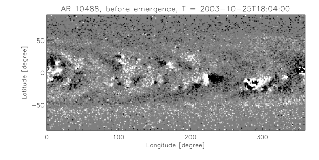
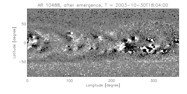
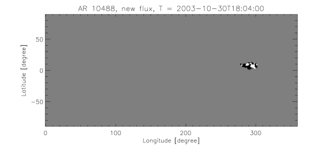
Figure 1: Surface radial magnetic field maps — pseudo-magnetograms — from the LMSAL forecast model show the pre-emergence global field (top row), the post-emergence global field (middle row), and the extracted new flux (bottom row) added to the global field by the emergence of AR 10488. White/black are outward/inward radial flux densities, respectively; grayscale saturation is set to $\pm 20~{}{\rm Mx}\cdot{\rm cm}^{-2}$.

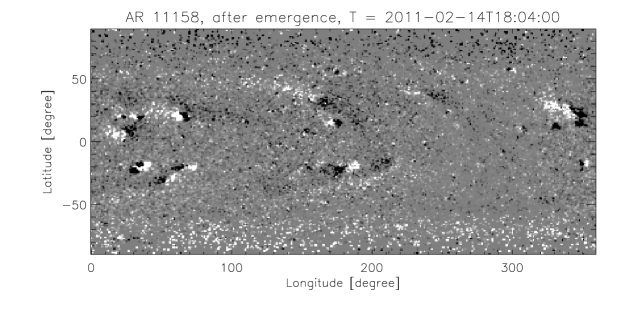
Figure 2: As in previous figure, surface radial magnetic field maps showing the pre-emergence global field (top row), the post-emergence global field (middle row), and the extracted new flux (bottom row), in this case from the emergence of AR 11158.

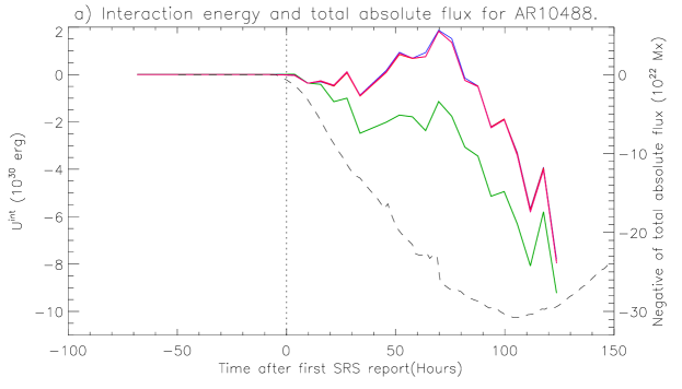
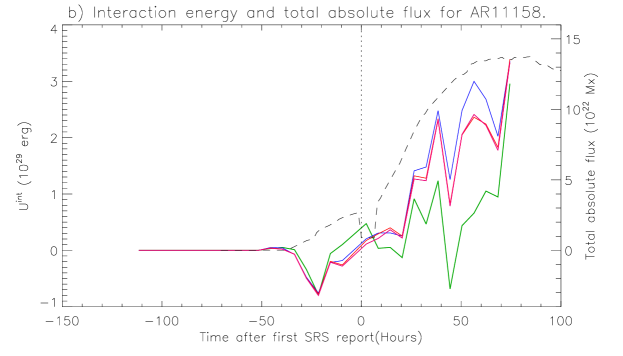
Figure 3: Plots of interaction energies (solid lines) and total unsigned magnetic fluxes (dashed) for AR 10488 (left) and AR 11158 (right). Solid lines represent the result for $U^{\rm int}$ with maximum $\ell$ values of 32, 64, 128 and 256 in the spherical harmonic transforms, and are colored green, blue, pink, and red respectively. It can be observed that the curves converge with a increasing resolution (higher $\ell_{\rm max}$); most nearly overlap in the 10488 case. The disagreement between the total unsigned flux and $U^{\rm int}$ curves implies that $U^{\rm int}$ is not trivially related to total flux.

Figure 3 shows the time variation of total unsigned flux and interaction energy $U^{\rm int}$ as the emergence proceeds in each region. One can see that $U^{\rm int}$ does not depend trivially on the total unsigned flux: while both quantities tend to grow with the emergence, they do not agree closely. From this, we conclude that the interaction energy depends on magnetic structure that is not simply related to the total unsigned magnetic flux.

The behavior of $U^{\rm int}$ in the regions differs: it swings strongly negative in AR 10488, but stays mostly positive in AR 11158. While both AR 10488 and AR 11158 produced large flares, we are interested in flare activity in their neighbors. Given AR 10488’s negative interaction energy, the presence of global free energy due to this emergence is indicated. Its nearest neighbor, AR 10486, produced several large flares; we do not know, however, whether those flares were triggered by the emergence of AR 10488. In addition, we faced a practical problem when computing the interaction energies due to the emergence of AR 10488: magnetic flux from far-side PEARs was rotating around the Sun’s east limb in the interval over which we computed interaction energies, and was steadily incorporated into the potential field computations. These other “new” active regions confound unambiguous attribution of the negative interaction energy to the emergence of AR 10488. (Given the lack of “$4\pi$” observations of the Sun’s photospheric magnetic field, all coronal field models will unavoidably suffer from similar deficiencies.) In contrast, AR 11158 did not exhibit a negative interaction energy; and its nearest neighbor, AR 11156, did not produce any significant flares during the interval that we studied (only two B-class flares). While the behavior of the neighbors of ARs 10488 and 11158 is consistent with our expectations based upon their interaction energies, a statistical investigation of interaction energies and simultaneous flare activity would be needed to draw any conclusions about whether interaction energies are significantly associated with flaring.

We note, however, that the values we find for $U^{\rm int}$ in both cases (of order 10²⁹ - 10³⁰) are relatively small compared to the energy released in large flares and CMEs, which often exceed 10³² erg (e.g., Emslie et al. 2012). Both of these cases involved relatively large active regions emerging near PEARs, so the interaction energies we find are probably large compared what would be found for more typical emerging regions. Given that the values of the interaction energies we find are far below the estimated energies released in relatively large flares, it is possible that the interaction energies computed in our approach do not quantify any significant physical property associated with flare activity. We expect that global, time-dependent models of non-potential structures in coronal magnetic fields (e.g., Yeates, Mackay, and van Ballegooijen 2008, or a larger-scale version of the model developed by Cheung and DeRosa 2012) could more accurately capture the energetic coupling between active regions, albeit at considerably greater computational expense than our approach.

3 Emerging Regions & Flaring Rates

Despite of the shortcomings in our interaction-energy approach for estimating the energetic consequences of new-region emergence, we still expect that the emergence of new regions can create additional topological free magnetic energy in the corona. As noted above, this is because the global magnetic connections in the actual post-emergence magnetic field will initially differ significantly from the potential post-emergence magnetic field. This change in free energy introduced by new emerging region could result in an increase of flares in PEARs.

3.1 Estimating emergence times

To associate flares in PEARs with a new active region’s emergence, it is first necessary to specify an emergence time for the new region. For this purpose, we developed two different sets of new-region emergence times, which trade off accuracy for the number of available cases.

The first and most direct source of estimated emergence times is the SRS records. We have such records from 1996 to the present, typically produced at at 00:30UT every day. The date of the earliest report of each active region then gives a rough estimate for its emergence time. As will be shown, this often agrees to within 24 hours of a more precisely determined emergence time. Using the SRS emergence time has two disadvantages. First, the record for each active region starts when human observers recognize the new flux system as an active region, so it is typically delayed by one day or two after the first appearance of new flux (Leka et al., 2013), and the threshold for recognition of new flux as an active region is unclear. Further, as noted by Dalla, Fletcher, and Walton (2008), there is a detection bias in this catalog: new regions that emerge toward the limbs are often not immediately detected (by either human observers or algorithms, e.g., Watson et al. 2009), an issue we revisit briefly below. Second, the inherent time resolution is limited, because SRS reports are made only once every 24 hours.

Another way to get a more accurate emergence time for a new AR, with physically meaningful criteria, is to analyze the growth of the region’s magnetic flux in full-disk magnetograms of the line-of-sight field recorded by the Michelson-Doppler Interferometer (MDI) (Scherrer et al., 1995). These magnetograms have 2” , pixels, and were nominally recorded at 96-minute cadence.

To analyze a given emergence, we must identify all pixels with associated with a new region as it emerges. For a sample of 186 emergence events near disk center (within 45^∘), we developed an automated procedure to do so. Starting from a region’s first appearance in an SRS report, we extract a sequence of magnetograms from 72 hours before to 72 hours after the SRS appearance, under the assumption that flux might have been present before the new region was recognized by the observers that compile the SRS reports. We then estimate the region’s location at each time in the sequence, based upon its position in the initial SRS report. We smooth each magnetogram with a 6-pixel wide, square spatial boxcar, and then attempt to determine which magnetic flux in the neighborhood of the new region’s location “belongs” to the new region — versus being simply noise, or belonging to a PEAR. We do so by identifying all groups of contiguous, above-threshold pixels, using the label_region algorithm native to IDL. To exclude noise when relatively little flux has emerged, we only group pixels with absolute LOS magnetic field, $|B_{\rm LOS}|,$ above a more restrictive threshold $40~{}{\rm Mx}\cdot{\rm cm}^{-2}$ (cf., $15~{}{\rm Mx}\cdot{\rm cm}^{-2}$ used previously, for mature active region fields in the lower-resolution LMSAL forecast model). We then associate groups of pixels that are among both (i) the three closest and (ii) the three largest with the new region. To avoid including flux from other active regions in this patch, we exclude areas closer to the time-adjusted SRS-reported position of any PEARs than to the new region’s time-adjusted location. To produce a time series of flux associated with the new region, we then sum the unsigned LOS flux in all groups of pixels that belong to the new region. Since we are primarily concerned with short-timescale, relative changes in new-region flux, we did not correct pixel areas for foreshortening.

As an example of the method, in Figure 4, we show four MDI magnetograms of AR 11158, with contours outlining flux associated with the new region. The first three magnetograms show the growth of the region during its initial emergence phase, on 2011-02-11. The final magnetogram shows the region at the start of 2011-02-15, after most of its flux has emerged, about 100 minutes before the start of the X2.2 flare. Between the first and second frames, an initially ungrouped emerging bipole is subsequently grouped with the new region as the bipoles grow toward each other. As noted above, this region experienced a more rapid phase of emergence that began around 18:00 UT on 2011-02-12 (Chintzoglou and Zhang, 2013), which is shown in the bottom panel of Figure 3.

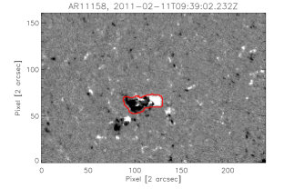
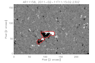
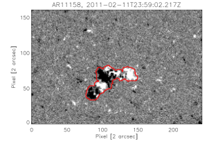
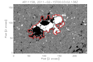
Figure 4: Magnetograms of AR 11158, with contours showing flux associated with the emerging region. Between the top-left and top-right magnetograms, an initially ungrouped emerging bipole becomes grouped with the region, as the emerging bipoles grow toward each other. The bottom-right magnetogram shows the region after nearly all of its flux has emerged, about 100 minutes before the X2.2 flare.

In practice, we find that this automated approach can sometimes fail to properly identify pixels associated with a given new region, typically for a few consecutive magnetograms. This can cause transient dips in flux (e.g., Figure 5d). In most cases, however, it performs well enough: in our sample of 186 emergence events, we manually rejected 70 for having unphysical jumps in the flux-versus-time curves due to poor flux attribution. Although the method is imperfect, we did not invest further effort to optimize it, since we only use this tool in an ancillary investigation of emergence times.

a)
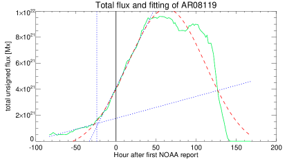
b)
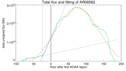
c)
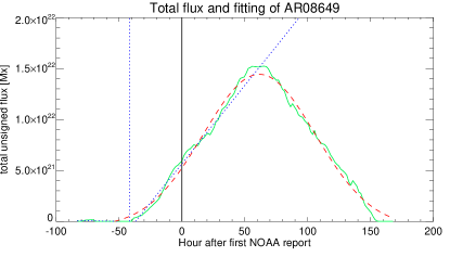
d)

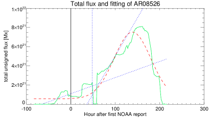
Figure 5: Examples of curve fitting of total unsigned flux to find emergence time. Green lines in all panels show flux versus time in a given emergence region. Red dashed lines show a Gaussian fit to the flux profile. The tilted dotted lines represent the two-slope, piece-wise continuous linear fits to the start of the flux-versus-time curve, while the vertical dotted line shows the emergence time determined from these fits, set by the gradual-to-rapid transition in the rate of emergence. Vertical solid lines (always at zero) show the time of each region’s first SRS report. Panels a) and b) show examples of regions with two-phase emergence; the gradual-to-rapid emergence transition is smooth in the former, but more sudden in the latter. The latter behavior was more common in the regions we studied. Panel c) shows a region with a single emergence phase; the fitted, pre-emergence slope is zero. Panel d) shows a case in which our flux identification algorithm failed, for a subset of time steps, to consistently determine which magnetogram flux “belongs” to the new AR (versus nearby PEARs, or the background) during the emergence.

We chose to define the start of a region’s emergence to be at the break point of a two-slope, piece-wise continuous linear fit to its flux-versus-time curve. This approach grew out of our observation that in many regions (e.g., AR 11158), flux (as identified by our algorithm) emerges in two phases: an initial, gradual phase, followed by a phase of more rapid emergence (e.g., Figure 5, panels a and b). The location of the break point between the two linear fits was selected to minimize the summed squared error in the overall fit. The start of the fitting interval was 84 hours prior to the first SRS report containing the new region. We set the endpoint of the time interval for our curve fitting to be the earlier of either (i) the time of the first NOAA record or (ii) the time at which the region reached 75% of its maximum unsigned flux. This guarantees that the flux curve to be fitted is almost linear after the turning point, so the piece-wise linear fit finds the dramatic change of flux growth well. We treat this turning point as the emergence time, since in many cases it captures the start of significant emergence. We also found many regions in which flux emerges at a single, roughly constant rate, and this fitting procedure also works well for such cases; the slope for the pre-emergence interval is simply zero (Figure 5c).

Table 1: For each emerging region that we study, we show the start and stop times of our fitting interval, and the two slopes found by our algorithm.

NOAA	SRS Appearance	Fitted Appearance	Init. Slope $a_{1}$	Final Slope, $a_{2}$
AR #	[YYYY-MM-DD hh:mm]	[YYYY-MM-DD hh:mm]	[2 $\times 10^{16}$ Mx/s]	[2 $\times 10^{16}$ Mx/s]
7982	1996-08-08 00:00	1996-08-08 17:36	1.56	6.11
8119	1997-12-09 00:00	1997-12-08 00:03	0.97	7.18
8169	1998-02-28 00:00	1998-02-26 11:12	0.00	3.95
8193	1998-04-05 00:00	1998-04-04 06:24	4.55	28.28
8200	1998-04-10 00:00	1998-04-08 19:12	1.04	11.62
8203	1998-04-15 00:00	1998-04-14 11:15	0.57	17.19
8226	1998-05-24 00:00	1998-05-23 03:11	0.54	26.55
8404	1998-12-07 00:00	1998-12-05 20:48	0.70	20.13
8506	1999-04-04 00:00	1999-04-03 11:12	2.32	17.91
8562	1999-06-01 00:00	1999-05-31 00:00	2.31	23.67
8582	1999-06-12 00:00	1999-06-10 14:24	0.25	7.85
8649	1999-07-28 00:00	1999-07-26 06:24	-0.13	8.80
8737	1999-10-20 00:00	1999-10-18 06:23	1.14	10.69
8743	1999-10-26 00:00	1999-10-29 04:48	2.00	11.22
8757	1999-11-06 00:00	1999-11-05 11:12	0.55	10.31
8797	1999-12-14 00:00	1999-12-12 11:11	0.74	7.04
8837	2000-01-19 00:00	2000-01-17 07:59	0.00	13.51
8844	2000-01-25 00:00	2000-01-24 11:11	0.72	21.53
8897	2000-03-02 00:00	2000-03-02 03:15	0.66	6.31
8904	2000-03-09 00:00	2000-03-09 03:11	3.20	18.24
8917	2000-03-19 00:00	2000-03-18 04:47	0.00	17.03
8918	2000-03-20 00:00	2000-03-19 03:11	1.41	13.83
8926	2000-03-24 00:00	2000-03-22 19:15	0.23	12.71
8935	2000-03-30 00:00	2000-03-27 22:23	0.09	7.42
8968	2000-04-20 00:00	2000-04-19 11:15	0.99	15.00
9135	2000-08-16 00:00	2000-08-13 17:35	1.84	11.99
9136	2000-08-18 00:00	2000-08-16 11:12	-0.25	16.51
9139	2000-08-21 00:00	2000-08-19 14:23	0.84	14.21
9144	2000-08-26 00:00	2000-08-25 04:47	0.26	24.74
9170	2000-09-22 00:00	2000-09-20 01:35	0.00	10.21
9290	2000-12-28 00:00	2000-12-27 19:11	3.18	12.22
9291	2000-12-30 00:00	2000-12-28 15:59	0.06	8.84
9324	2001-01-24 00:00	2001-01-21 16:03	0.00	2.54
9366	2001-03-03 00:00	2001-02-28 23:59	0.48	8.02
9408	2001-03-29 00:00	2001-03-27 08:03	0.07	12.38
9413	2001-04-02 00:00	2001-03-31 22:24	0.13	7.45
9426	2001-04-12 00:00	2001-04-10 19:12	1.25	15.31
9432	2001-04-19 00:00	2001-04-17 11:12	1.12	9.72
9447	2001-05-01 00:00	2001-05-01 04:48	2.79	13.57
9455	2001-05-12 00:00	2001-05-10 11:12	0.35	18.01
9484	2001-06-02 00:00	2001-06-01 16:00	0.63	17.62
9512	2001-06-22 00:00	2001-06-21 12:51	3.55	17.56
9531	2001-07-09 00:00	2001-07-07 14:24	0.25	21.83
9553	2001-07-24 00:00	2001-07-23 04:51	0.75	10.76
9574	2001-08-11 00:00	2001-08-10 07:59	1.42	40.42
9611	2001-09-08 00:00	2001-09-07 08:03	0.37	9.35
9631	2001-09-21 00:00	2001-09-19 16:03	0.70	13.71
9635	2001-09-24 00:00	2001-09-22 20:48	0.22	5.94
9639	2001-09-27 00:00	2001-09-26 16:03	1.95	7.40
9645	2001-10-02 00:00	2001-09-30 04:47	-0.14	7.90
9674	2001-10-20 00:00	2001-10-19 12:51	1.55	34.59
9692	2001-11-08 00:00	2001-11-07 06:23	1.84	26.65

Table 2: Continuation of Table 1.

NOAA	SRS Appearance	Fitted Appearance	Init. Slope $a_{1}$	Final Slope, $a_{2}$
AR #	[YYYY-MM-DD hh:mm]	[YYYY-MM-DD hh:mm]	[2 $\times 10^{16}$]	[2 $\times 10^{16}$]
9719	2001-11-29 00:00	2001-11-26 15:59	1.92	0.38
9739	2001-12-14 00:00	2001-12-13 11:15	-0.12	14.79
9748	2001-12-21 00:00	2001-12-20 14:23	0.50	15.29
9764	2001-12-29 00:00	2001-12-29 22:23	2.14	12.51
9768	2002-01-02 00:00	2002-01-03 17:39	3.56	11.71
9786	2002-01-17 00:00	2002-01-16 01:39	0.83	4.05
9844	2002-02-24 00:00	2002-02-23 03:12	1.21	8.82
9846	2002-02-25 00:00	2002-02-24 08:00	-0.06	12.72
9868	2002-03-12 00:00	2002-03-10 14:24	1.64	7.67
9872	2002-03-16 00:00	2002-03-14 16:00	0.78	7.49
9873	2002-03-18 00:00	2002-03-16 04:48	3.51	15.43
9912	2002-04-19 00:00	2002-04-18 03:12	1.47	14.55
9926	2002-04-28 00:00	2002-04-25 03:11	23.27	5.99
9931	2002-05-02 00:00	2002-04-30 06:23	0.02	6.85
10045	2002-07-25 00:00	2002-07-25 03:15	1.74	17.88
10050	2002-07-27 00:00	2002-07-26 22:23	1.77	30.38
10072	2002-08-12 00:00	2002-08-11 06:27	0.33	6.73
10097	2002-09-01 00:00	2002-08-30 15:59	1.00	6.06
10099	2002-09-02 00:00	2002-09-01 01:35	0.35	8.12
10109	2002-09-11 00:00	2002-09-09 17:35	1.26	6.74
10110	2002-09-11 00:00	2002-09-09 09:35	1.03	6.88
10132	2002-09-23 00:00	2002-09-21 09:36	-0.14	15.09
10133	2002-09-24 00:00	2002-09-22 03:11	0.00	7.57
10178	2002-11-01 00:00	2002-10-30 19:11	0.44	11.24
10188	2002-11-07 00:00	2002-11-06 04:51	1.22	16.76
10227	2002-12-14 00:00	2002-12-13 08:03	0.00	5.31
10249	2003-01-08 00:00	2003-01-06 16:02	0.88	7.51
10253	2003-01-11 00:00	2003-01-09 23:59	0.00	9.02
10313	2003-03-14 00:00	2003-03-12 20:48	0.00	11.24
10350	2003-04-30 00:00	2003-04-28 09:36	-0.45	66.56
10381	2003-06-10 00:00	2003-06-09 16:02	0.95	10.29
10382	2003-06-11 00:00	2003-06-09 19:14	0.01	3.88
10388	2003-06-20 00:00	2003-06-19 07:58	2.66	16.20
10491	2003-10-28 00:00	2003-10-26 14:23	0.00	10.43
10591	2004-04-13 00:00	2004-04-11 03:15	0.00	5.39
10601	2004-05-01 00:00	2004-04-30 01:35	0.67	15.48
10605	2004-05-05 00:00	2004-05-03 12:47	0.62	7.67
10692	2004-10-25 00:00	2004-10-23 17:36	0.01	13.14
10747	2005-04-01 00:00	2005-04-01 19:11	1.03	8.57
10770	2005-05-30 00:00	2005-05-28 23:59	0.13	6.85
10819	2005-11-01 00:00	2005-10-30 14:24	1.36	5.04
10862	2006-03-19 00:00	2006-03-16 16:03	-0.35	5.01
10869	2006-04-07 00:00	2006-04-05 01:35	0.00	4.63
10879	2006-05-03 00:00	2006-05-01 06:23	0.05	5.09
10885	2006-05-21 00:00	2006-05-19 03:11	0.02	4.04
10917	2006-10-20 00:00	2006-10-21 04:51	2.06	19.52
10955	2007-05-10 00:00	2007-05-08 11:11	2.06	6.52
11005	2008-10-12 00:00	2008-10-10 16:03	0.00	10.93
11027	2009-09-23 00:00	2009-09-22 01:39	0.27	11.39
11029	2009-10-24 00:00	2009-10-22 22:27	0.39	7.89
11061	2010-04-06 00:00	2010-04-05 09:39	1.32	19.72
11105	2010-09-03 00:00	2010-09-01 19:15	0.14	6.54

For the 116 emergence cases with smooth flux evolution, we deemed the fit results to be poor in 11 cases. In a further 5 cases, the initial part of the flux-versus-time plot was inconsistent with new flux emergence, being well above zero (indicating pre-existing flux) and either (i) decreasing or (ii) flat. Of the remaining 100 cases, we manually characterized 46 as being more consistent with single-phase emergence, and 54 as being more consistent with two-phase emergence. Hence, we find about 50% of emergence events exhibit two-phase behavior. Examples of single- and two-phase emergence events are shown in Figure 5.

We deemed our fitted slope break points to accurately capture the emergence time in 104 cases. (In one of the 105 well-fitted cases, the fitted lines approximately matched the overall flux-versus-time evolution, but the break point in slopes found by our algorithm occurred at a time that differed from the onset of clear emergence.) In the top panel of Figure 6, we plot a histogram of the time lags between our emergence time and the first appearance in the SRS reports, with positive corresponding to an earlier detection by our algorithm. A Gaussian fit (overplotted in blue) is centered at 26 hr, with a sigma of 15 hr. The distribution peaks near +24 hr, meaning our algorithm tends to define emergence times about a day ahead of regions’ appearances in SRS reports. This confirms a similar result reported by Leka et al. (2013). The distribution’s standard deviation is 12 hours, which shows that the SRS time is good as long as we do not go beyond its time resolution of one day. In Tables 1 and 2, we list the SRS and fitted appearance times for the 104 well-fitted regions, in which our fitting algorithm’s break point in slopes matched the onset of emergence. We also list the initial and final slopes during the fitting interval.

Leka et al. (2013) suggested a different definition for the emergence start time: the point at which a region’s total flux is 10% of the maximum over the lifetime of the region. However, at least with our imperfect computation of total flux, this 10% rule for many regions does not select a meaningful point for the start of emergence. As Figure 5 shows, 10% of the maximum flux may appear very early, when the uncertainty in the total flux is relatively large. Further, the exact maximum of a region’s unsigned flux can also be somewhat uncertain.

In the middle panel of Figure 6, we plot the histogram of the fraction of each region’s flux present at two possible definitions of appearance time (cf., emergence time): our break-point approach (in red) and the first-SRS time (in purple). Because a new region can appear at any time, but SRS reports are only issued once per day, the fraction of peak flux present at the first-SRS time is essentially random. In contrast, at the majority of two-slope break-point appearance times, less than 10% of regions’ flux has emerged. For comparison, the 10% cutoff is shown as a vertical, dashed line.

In the bottom panel of Figure 6, for two-phase events, we plot a histogram of the natural logarithms of ratios of slopes in the first and second phases, $a_{1}$ and $a_{2}$, respectively. The distribution is broad, with peak at $\log(a_{2}/a_{1})=2.2,$ corresponding to a ratio of slopes of more than 7 to 1 between the rapid and gradual phases.

While we believe the emergence times acquired from curve fitting are more accurate than those from SRS reports, NOAA’s SRS database provides a much larger amount of cases for statistical analyses. This is especially true when applying various thresholds on new active regions to consider, e.g., region size, or proximity to the nearest PEAR. We chose not to combine our set of fitted times with the larger set of SRS times, because doing so would make our emergence times inconsistent.

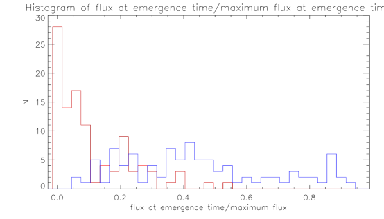
Figure 6: Top: The histogram of time differences between AR appearance times from the SRS reports and emergence times that we estimate from our fitted break point for the gradual-to-rapid transition in the unsigned flux curve. Positive times correspond to delayed appearance in the SRS reports. This histogram includes 104 active regions. Middle: The histogram of the fraction of total unsigned flux at the inferred time of emergence to the maximum total unsigned flux of each active region: red histogram is for our fitted emergence times, and purple is for appearance times in SRS reports. The dotted line shows the 10% threshold adopted by Leka et al. (2013). We see that in many cases, the fitting procedure determines emergence times prior to the 10% threshold. In contrast, SRS appearances are almost equally likely to occur at any fraction of a new region’s maximum flux. Bottom: This histogram shows the ratio between the rapid-phase and gradual-phase rates of flux emergence, on a natural log-linear axis, so greater than 0 means larger slope after emergence. This distribution peaks around 2.2, implying $a_{2}/a_{1}\,\lower 3.0pt\hbox{$\sim$}\hbox to0.0pt{\hss\raise 2.0pt\hbox{$>$}}\,7$.

3.2 Superposed Epoch Analysis of Flares and Emerging ARs

To quantitatively characterize the relationship between active region emergence and flaring in PEARs, we perform superposed epoch analysis on active region emergence events and flares. The idea of superposed epoch analysis (or Chree analysis) is to co-register the times of one set of events at a common, “key” time, and superpose the event counts for the other set of events relative to the co-registered key time. A peak at or near the key time would indicate a relation between these two sets of events. We define the key time to be the emergence of new active regions, and compute rates of flaring in PEARs relative to this key time.

For emergence times, we use the SRS reports: we treat a region’s first appearance in an SRS report as its emergence time. For regions that first appeared within 45 degrees of disk center, we then investigate flare activity in PEARs $\pm 72$ hours from this time using the GOES flare catalog. The maximum umbral area of new regions (also given in the SRS reports, with correction for foreshortening) is expected to be correlated with these regions’ total unsigned fluxes (e.g., Figure 4 of Fisher et al. 1998), and should thus be related to the strength of interaction between the new region and PEARs. New AR size therefore provides a plausible criterion to select sets of active regions to investigate for a dose-response relationship.

Figures 7 and 8 give our primary results regarding the influence of new regions on flaring in PEARs. In each panel of Figure 7, flaring rates for several GOES flare thresholds (all flares, C1, M1, M5, and X1) are shown with solid lines for seven 24-hour periods: $\pm 12$ hours from the first SRS report listing a new region, and $\pm$ 3 days on either side of this. These rates are in units of flares per day per $N$ emergence events, where $N$ is given at the top of each plot: the rate is computed by simply summing all flares for all emergence events, and dividing by seven. To fit rates for all thresholds on a single plot, the mean rate for each flare threshold over the entire 7-day interval was then scaled to one; the unscaled daily-average flare rate is given for each class next to that class’s label. Dotted lines show the mean rate $\pm$ 1-sigma expected uncertainty ranges (see below) in the flaring rate for each threshold, assuming that Poisson statistics govern the count rate, computed separately for the 3-day time periods before and after the key-time interval (and excluding the key-time interval itself).

To search for any evidence that PEAR flare rates depend upon new-region size, we computed their flare rates for three subsets of emergence events, with increasingly restrictive minimum thresholds on new regions’ umbral-area sizes. The top, middle, and bottom panels in Figure 7 show PEAR flare rates associated with emergence of new regions with peak umbral areas larger than 30, 75, and 110 micro solar hemispheres (MSH) or microhemispheres (mhs), respectively. While we expected larger new regions to more strongly affect PEARs flare rates than smaller new regions, we do not see clear evidence of this effect. One possible explanation for this lack of strong size dependence is that flare-relevant perturbations to PEARs’ magnetic environments might set in after only modest amounts of flux have emerged, so the later growth of regions to their peak sizes does not matter.

In all three panels of Figure 7, the fractional increase in the rate of more powerful flares is larger than increases in the rates of weaker flares. One possible explanation is obscuration, an effect pointed out by Wheatland (2001), who showed that the GOES catalog suffers from the tendency of the flare identification procedure to fail to identify relatively small flares that follow large flares. Small flares are also lost in the GOES background during very active periods (e.g., Hudson, Fletcher, and McTiernan 2014). Another plausible explanation is that the higher peak GOES X-ray flux necessary for a flare to be characterized as more powerful likely requires the involvement of magnetic fields over a larger area in the flare. Physically, this might mean more magnetic flux reconnects; observationally, this would in many cases produce flare ribbons sweeping over more photospheric magnetic flux, and post-flare loops over a larger area. Hence, larger flares are likely more non-local, i.e., they probably involve more global-scale magnetic connections relative to smaller flares. It can also be seen that the increases in flaring rates precede the time of the first SRS report by a few dozen hours, consistent with the delay in SRS reports noted above (and shown in the histogram in the top panel of Figure 6).

We included flares from PEARs any distance from new regions when computing the rates shown in Figure 7. To investigate whether PEARs in close proximity to new regions are more likely to flare, in the top panel of Figure 8, we plot PEAR flare rates for the subset of new regions that both (i) had peak umbral areas above 75 MSH in size and (ii) were less than 45^∘ from nearest PEAR. The peaks at the key time in this panel are larger than the peaks in the middle panel of Figure 7 (which has the same region-size threshold), implying that closer emergence events are more strongly assocated with increased flare activity. This is in accordance with expectations from our interaction-energy model, based upon the scaling of the potential field interaction with distance. Note also that for this set of PEARs close to the emerging region, the rates of all classes of PEAR flares increase. We remark that NOAA’s AR designations are somewhat subjective; some observers might characterize a new NOAA region close to a PEAR as emergence associated with that PEAR instead. To investigate this idea, in the middle panel of Figure 8, we plot histograms of distances to (i) PEAR flares of any class (green) and (ii) the nearest PEAR to the emergence of any region larger than 75 MSH. Both PEARs and flares are quite close to new regions in some cases, but in the majority of cases they are clearly separated.

In the bottom panel of Figure 8, we plot PEARs’ flare rates for the subset of new regions for which: (i) the break point in our two-phase linear fits to the flux-versus-time curves were deemed to match the region’s emergence time; and (ii) areas exceeded 75 MSH. Compared to the humps in flare rates found from the SRS appearance times, the onset of the flare rate increase shifted to the right, consistent with our expectation that the SRS appearance times are later than the true emergence by about 24 hr. Also, the peak for flares X1 and greater is higher than for the corresponding SRS-emergence plot (middle panel of Figure 7), which is consistent with more accurate estimation of the key times in our superposed epoch analysis.

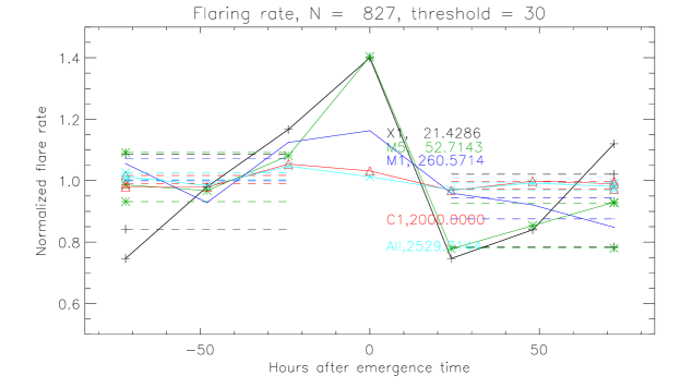
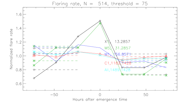
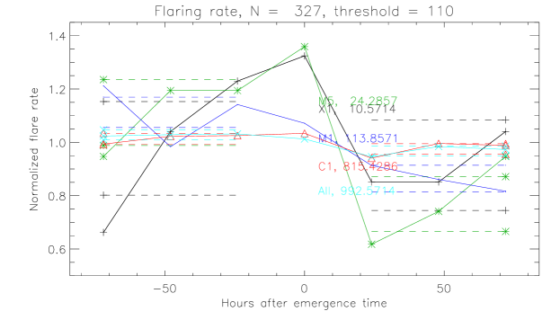
Figure 7: These plots show rates of flares in PEARs before and after the key time determined by new active region emergence. On each plot, each data point shows the normalized flare count rate, for several flare thresholds, summed over all key times, with each flaring rate scaled so that the mean rate is 1 over the 7-day interval shown. Symbols differ for each flare threshold: they are $\times,\triangle,$ dot (.), $*,$ and $+$, for all flares, C1, M1, M5, and X1, respectively. The actual mean rate (in units of flares per day per N emergence events) is annotated for each line. The dashed lines, marked by color and endpoint symbols, are mean rates $\pm$ 1-$\sigma$ uncertainty intervals for the 3 days before or after the key time, excluding the key-time interval itself (to better represent natural variations in the rate without the influence of the new active region). From top to bottom, only regions larger than increasing thresholds for new active region size (in micro solar hemispheres, or MSH) are included.

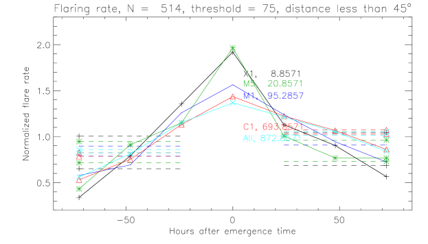
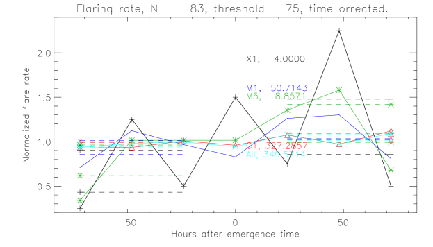
Figure 8: Top: rates of flares in PEARs, as in the previous figure, but including only flares from PEARs closer than 45 degrees from the newly emerged region’s location. Middle: histograms of flare distances (green) from each new region, and distances (red) to the nearest PEAR for each emergence. Bottom: flare rates of PEARs in the subset of active regions for which we determined an emergence time from the break-point approach.

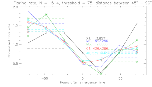
Figure 9: Rates of flares in PEARs between 45^∘ and 90^∘ from new regions. It exhibits a “U” shape, which can be understood from the distribution of recorded locations of spot-containing regions (middle panel), which shows fewer regions toward the limbs; for a point near disk center, there are relatively few PEARs $>45^{\circ}$ away, so the PEAR flare rate is lower. There is also an asymmetry in the top plot, with the left side higher, corresponding to more flares originating in west-disk PEARs. This is consistent with E-W biases (e.g., Dalla, Fletcher, and Walton 2008) in the distributions of both spot-containing regions (middle panel) and all NOAA regions (bottom panel; this includes H$\alpha$ plages without spots): fewer regions are identified on the eastern disk, so fewer east-disk flares are likely to be ascribed to any region.

While the increase in flares in PEARs closer than 45^∘ is evident, the rate on PEARs farther away is less clear. In the top panel of Figure 9, we show the rates of flares in PEARs between 45^∘ and 90^∘ from new emergences. To keep a uniform area that excludes beyond-limb regions, we only include regions in the half of the 90-degree circle centered on the new region that lies toward disk center and is bisected by the new region’s meridian. This implies that the initial three days of most regions’ histories involve westward PEARs, while the final three days of most regions’ histories involve eastward PEARs. The “U” shape of the rate curves can be understood from the distributions of recorded locations of spot-containing regions (middle panel), which show a relative dearth of regions toward the limbs: for points toward $75^{\circ}$ in either E or W longitude, there are more regions 45^∘ - 90^∘ away than there are for points near disk center. Hence, over each 7-day interval used in our superposed epoch analysis, the likelihood of flares from PEARs 45^∘ - 90^∘ away is highest at points away from disk center. There is also an asymmetry in the top plot, with the left side higher, corresponding to more flares originating in west-disk PEARs. This is consistent with E-W biases in the distributions of both spot-containing regions (middle panel) and all NOAA regions (bottom panel, which also includes H$\alpha$ plage regions lacking sunspots): fewer regions are identified on the eastern disk, so fewer east-disk flares are likely to be ascribed to any region. This E-W bias was previously reported by Dalla, Fletcher, and Walton (2008).

3.3 Significance of Flaring Rate Variations

To characterize the significance of variations in flaring rates associated with the emergence of new regions, we estimate the random rate variations that would be expected under the null hypothesis, i.e., that the emergence of new regions does not have any effect on flaring in PEARs. To do so, we separately estimated the flare rate and its uncertainty for the three-day intervals before and after the key time. Within each three-day interval, we treat the $j$-th day’s flare count, $n_{j}$, as a separate estimate of the average flare rate $\langle n_{f}\rangle$ per day per $N$ emergence events, with

$$\langle n_{f}\rangle=\frac{1}{J}\sum_{j=1}^{J}n_{j}~{},$$ (18)

for observations over $J$ days. Given the delay in appearance times in NOAA SRS reports relative to emergence times that we found from flux-versus-time curves (see the top panel of Figure 6 above), we expect that our pre-appearance flaring rate for SRS key times will be partially “contaminated” by new-region flux. To the extent that emergences do indeed increase the PEAR flaring rate, this contamination will increase the apparent background PEAR flaring rate, complicating the task of showing an increase above background associated with the new region. This is a price we have agreed to pay to increase our sample size with the SRS dataset.

We then assume Poisson statistics govern fluctuations in each day’s estimate of the flare rate, i.e., given $n_{j}$ flares on day $j$, the standard deviation in that day’s rate estimate is $\sqrt{n_{j}}$. For $J$ successive days of observations, we take the standard error in the mean flare rate, $\sigma_{f}$,

$$\frac{1}{\sigma_{f}^{2}}=\frac{J}{\langle n_{f}\rangle}~{},$$ (19)

as the uncertainty.

These averages and standard deviations in PEAR flare rates are used in Figures 7 and 8. In all plots of flare rates, solid lines show the flare rate for each flare threshold, normalized to make each threshold’s mean daily rate over the full, 7-day interval equal to unity. The dashed lines show $\langle n_{f}\rangle\pm\sigma_{f}$, where $\langle n_{f}\rangle$ and $\sigma_{f}$, where computed separately over the three-day pre- and post-emergence intervals.

We computed separate pre- and post-emergence uncertainty estimates on the flare rates for two reasons. First, as noted above, the GOES catalog suffers from obscuration. If new-region emergence does trigger flares in PEARs, some of which are large, then the subsequent PEAR rate for smaller flares will be systematically diminished by obscuration. Second, on physical grounds, the flare rate in PEARs might be suppressed after a large flare happens, since the large-scale, post-flare magnetic field should be in a more-relaxed state. We refer to this possible phenomenon as “flare shadows,” based upon the analogous effect in terrestrial geology, “stress shadows” (e.g., Mallman and Parsons 2008), in which most faults near one that just produced an earthquake are de-stressed. In the coronal magnetic field, separators play the role of terrestrial faults. While Wheatland (2001) showed convincing evidence that obscuration affects flare counts in the GOES catalog, this by itself does not rule out the existence of flare shadows.

Although essentially all of our flare rate plots exhibit noticeable peaks near the key time for M- and X-class flares, most peaks are basically 2$\sigma_{f}$ or less above the mean rate. Exceptions are for X1 and M5 or greater flares from any PEARs, all classes of flares from close PEARs (top panel of Figure 8), and for X1 or greater flares in PEARs for the subset of new regions in which we estimated the emergence time from the flux-versus-time curve (bottom panel of Figure 8), all of which are near 3$\sigma_{f}$ enhancements. We therefore characterize the effect for large flares as statistically significant: the emergence of new regions is associated with increases in the rate of large flares in all PEARs, and the rate of all classes of flares for PEARs close to the emerging regions. Given the relatively small numbers of large flares, however, the possibility that the peaks that we see arose from statistical fluctuations must be kept in mind.

4 Conclusions

In this paper we studied the influence of newly emerging active regions on flaring rates in PEARs.

We first presented a theoretical approach, based upon an interaction energy between new and pre-existing regions defined in terms of pre- and post-emergence potential fields. This interaction energy depends upon the part of potential field energy arising from coupling between pre-existing flux systems and the new active region. This term should generally not be a trivial replication of a new region’s total unsigned flux, as we have shown in case studies of two regions, AR 10488 and AR 11158, that emerged near pre-existing regions. We argue that, based upon Hale’s law, this interaction energy should often be negative, and that when negative it implies the presence of free energy in the coronal field as a result of the new region’s emergence. We use the term topological free energy to refer to free energy associated with a negative interaction energy between a new region and PEARs, as distinct from the internal free energy within each flux system. In our two case studies, the system we found to possess topological free energy, the AR 10488/AR 10486 pair, the nearby PEAR (10486) produced a large flare; our approach did not find topological free energy in the other system (AR 11158/11156), and the nearby PEAR (11156) did not produce any large flare.

We found, however, that even when a big, new region emerges very near another large PEAR, the interaction energy turns out to be relatively small compared to the energy released in large flares. Thus we conclude that this interaction energy cannot directly explain the energy released in subsequent flares. Instead, we suggest that the interaction energy might quantify the strength of the perturbation to the magnetic environment of PEARs — and if a given PEAR is only marginally stable, a larger interaction energy should imply a greater likelihood of a flare. In this view, new region emergence might trigger flares or CMEs by processes such as breakout reconnection (Antiochos, DeVore, and Klimchuk, 1999) between overlying fields in the old flux system and the new flux system, enabling stressed, inner fields in the old flux system to erupt. We believe that more involved analyses of the magnetic interactions between new and old regions using potential fields — such as those undertaken by Longcope et al. (2005), Tarr and Longcope (2012), and Tarr et al. (2014) — can provide much more information than our interaction-energy approach, although only with greater effort.

We then undertook a statistical study of the rates of flares in PEARs near the times at which new regions emerged, using superposed epoch analysis. Our results suggest that the emergence of new regions is associated with increases in the rate of flares in PEARs, especially M- and X-class flares, with the size of the effect on the flare rate being 2$\sigma_{f}$ or more. Relatively little influence of new-region emergence on the rates of smaller flares in PEARs was found, except for PEARs within 45^∘ of new regions. This is perhaps because smaller flares might arise from local magnetic field structure and processes that are less influenced by changes in the large-scale structure of the coronal magnetic field. Dalla, Fletcher, and Walton (2007) investigated flare rates associated with new regions that emerged within 12^∘ of a PEAR, but found only a relatively small increase in the flare rate averaged over the 4 days following the emergence times. We note that the rate increases that we find using SRS reports typically start about one day before this “emergence time,” and only last about one day afterward. Hence, the effects we see could be substantially diminished in 4-day averages of post-SRS flare rates.

We believe that the statistical association between new-region emergence and temporary enhancements in the rate of remote flaring that we report arises from large-scale magnetic interactions between each new region and PEARs in the corona. Our observations, however, only demonstrate correlation, not causation. So it is possible that some other physical process(es) explains the correlation.

One possible alternative explanation is the organization of magnetic fields at super-active-region scales, in “activity complexes” (Bumba and Howard, 1965) or “activity nests” (Schrijver and Zwaan, 2000). It is well known that new flux is much more likely to emerge within PEARs (e.g., Liggett and Zirin 1985; Harvey and Zwaan 1993), and observations show that flares within a PEAR tend to be associated with emergence of additional flux within that PEAR (e.g., Martin et al. 1982). It is possible that there exists some physical connection, through the solar interior, between the emergence of (i) additional within PEARs and (ii) new flux that forms a new AR. Such coordinated emergence could produce correlations like those we report. The necessary length scale of such super-active-region connections can be inferred from the red histogram in middle panel of Figure 8, which shows the distribution of distances to the nearest PEAR for each emergence. The bulk of new emergences in our are farther than 15 heliocentric degrees (i.e., greater than 180 Mm) from pre-existing regions.

In our view, observations of enhanced flare activity in PEARs due to the emergence of new regions have clear implications for understanding the release of magnetic energy in flares and CMEs. Foremost, interactions between coronal magnetic flux systems are often global in scale: evolution in one part of the corona can drive evolution in distant regions. This idea is not new, and has been discussed by many other researchers. Examples include the contexts of emergence-triggered filament disruptions (e.g., Bruzek 1952; Feynman and Martin 1995), transequatorial loop systems observed with the soft X-ray telescope aboard the Yohkoh satellite (Pevtsov, 2000), PFSS models of the implications of AR orientation with respect to the background coronal field (Luhmann et al., 2003), and sympathetic flaring (e.g., Moon et al. 2002; Schrijver and Title 2011). Our results are another manifestation of this global-scale coupling.

These considerations are clearly relevant for space weather forecasting, since far-side evolution might have implications for front-side events, which can be geoeffective: What you don’t know can hurt you! In particular, geoeffective front-side flares and CMEs might be arise from processes associated with beyond-limb flux emergence. Currently, new-region emergence on the far side can be detected and calibrated in terms of total unsigned flux using helioseismology (e.g., González Hernández, Hill, and Lindsey 2007) and / or by combining STEREO EUV observations of emergence (e.g., Liewer et al. 2014) with known scalings between magnetic flux and EUV radiance (Fludra and Ireland, 2008). Our results motivate satellite missions enabling full-Sun (or “4$\pi$”) observations of the solar surface and atmosphere, for reasons both practical (to better predict space weather) and scientific (to better understand large-scale magnetic connections and their implications). In addition, for simulation efforts to understand active-region evolution (e.g., Cheung and DeRosa 2012), neglect of active regions’ global magnetic environment might ignore the crucial role of global-scale connections.

Beyond our main results, our efforts to objectively estimate active region emergence times from magnetograms led to an additional finding: many active regions (about half in our sample) exhibit “two-phase” emergence, with a phase of relatively gradual emergence followed by a relatively sudden change to more rapid emergence. We find that a piece-wise linear fit to the time profile of total unsigned magnetic flux captures this transition in the dynamics of emergence in many regions. Two-phase emergence has been seen in simulations of flux emergence, as in the modeling undertaken by Toriumi and Yokoyama (2011), who found that the rate of emergence in a single emerging flux structure varied with time as the structure reached the photosphere. In contrast, Chintzoglou and Zhang (2013) believe the gradual-to-rapid emergence in their observations of AR 11158 arose because the emerging structure was fragmented, with a weaker-field structure preceding a stonger-field structure. Further study of flux-versus-time profiles in models and observations is warranted.

While previous authors (Leka et al., 2013) defined emergence times from the appearance of 10% of the (subsequent) maxima of regions’ total unsigned flux, we argue that defining the emergence time from the fitted emergence rate — and perhaps at the transition point from gradual to rapid — is more robust to fluctuations (from noise or other artifacts) in the observed total unsigned flux, and captures an important physical aspect of the emergence process. As another by-product, we found reports of new active regions in NOAA’s Solar Region Summaries typically occurred about 24 hours after the actual start of significant new flux emergence, in agreement with previous reports (Leka et al., 2013).

References

- Altschuler and Newkirk (1969) Altschuler, M.D., Newkirk, G.: 1969, Magnetic fields and the structure of the solar corona. Solar Phys. 9, 131 – 149.
- Antiochos, DeVore, and Klimchuk (1999) Antiochos, S.K., DeVore, C.R., Klimchuk, J.A.: 1999, A Model for Solar Coronal Mass Ejections. ApJ 510, 485 – 493.
- Balasubramaniam et al. (2011) Balasubramaniam, K.S., Pevtsov, A.A., Cliver, E.W., Martin, S.F., Panasenco, O.: 2011, The Disappearing Solar Filament of 2003 June 11: A Three-body Problem. Astrophys. J. 743, 202. doi:10.1088/0004-637X/743/2/202.
- Bruzek (1952) Bruzek, A.: 1952, Über die Ursache der ”Plötzlichen” Filamentauflösungen. Mit 4 Textabbildungen. ZAp 31, 99.
- Bumba and Howard (1965) Bumba, V., Howard, R.: 1965, Large-Scale Distribution of Solar Magnetic Fields. Astrophys. J. 141, 1502. doi:10.1086/148238.
- Cheung and DeRosa (2012) Cheung, M.C.M., DeRosa, M.L.: 2012, A Method for Data-driven Simulations of Evolving Solar Active Regions. Astrophys. J. 757, 147. doi:10.1088/0004-637X/757/2/147.
- Chintzoglou and Zhang (2013) Chintzoglou, G., Zhang, J.: 2013, Reconstructing the Subsurface Three-dimensional Magnetic Structure of a Solar Active Region Using SDO/HMI Observations. Astrophys. J. Lett. 764, L3. doi:10.1088/2041-8205/764/1/L3.
- Dalla, Fletcher, and Walton (2007) Dalla, S., Fletcher, L., Walton, N.A.: 2007, Flare productivity of newly-emerged paired and isolated solar active regions. Astron. Astrophys. 468, 1103 – 1108. doi:10.1051/0004-6361:20077177.
- Dalla, Fletcher, and Walton (2008) Dalla, S., Fletcher, L., Walton, N.A.: 2008, Invisible sunspots and rate of solar magnetic flux emergence. Astron. Astrophys. 479, L1 – L4. doi:10.1051/0004-6361:20078800.
- Dove et al. (2011) Dove, J.B., Gibson, S.E., Rachmeler, L.A., Tomczyk, S., Judge, P.: 2011, A Ring of Polarized Light: Evidence for Twisted Coronal Magnetism in Cavities. Astrophys. J. Lett. 731, L1. doi:10.1088/2041-8205/731/1/L1.
- Emslie et al. (2012) Emslie, A.G., Dennis, B.R., Shih, A.Y., Chamberlin, P.C., Mewaldt, R.A., Moore, C.S., Share, G.H., Vourlidas, A., Welsch, B.T.: 2012, Global Energetics of Thirty-eight Large Solar Eruptive Events. Astrophys. J. 759, 71. doi:10.1088/0004-637X/759/1/71.
- Feynman and Martin (1995) Feynman, J., Martin, S.F.: 1995, The initiation of coronal mass ejections by newly emerging magnetic flux. J. Geophys. Res. 100, 3355 – 3367. doi:10.1029/94JA02591.
- Fisher et al. (1998) Fisher, G.H., Longcope, D.W., Metcalf, T.R., Pevtsov, A.A.: 1998, Coronal heating in active regions as a function of global magnetic variables. ApJ 508, 885 – 898.
- Fludra and Ireland (2008) Fludra, A., Ireland, J.: 2008, Radiative and magnetic properties of solar active regions. I. Global magnetic field and EUV line intensities. Astron. Astrophys. 483, 609 – 621. doi:10.1051/0004-6361:20078183.
- Forbes (2000) Forbes, T.G.: 2000, A review on the genesis of coronal mass ejections. JGR 105, 23153 – 23166.
- Freeland and Handy (1998) Freeland, S.L., Handy, B.N.: 1998, Data Analysis with the SolarSoft System. Solar Phys. 182, 497 – 500. doi:10.1023/A:1005038224881.
- Georgoulis, Titov, and Mikić (2012) Georgoulis, M.K., Titov, V.S., Mikić, Z.: 2012, Non-neutralized Electric Current Patterns in Solar Active Regions: Origin of the Shear-generating Lorentz Force. Astrophys. J. 761, 61. doi:10.1088/0004-637X/761/1/61.
- González Hernández, Hill, and Lindsey (2007) González Hernández, I., Hill, F., Lindsey, C.: 2007, Calibration of Seismic Signatures of Active Regions on the Far Side of the Sun. Astrophys. J. 669, 1382 – 1389. doi:10.1086/521592.
- Harvey and Zwaan (1993) Harvey, K.L., Zwaan, C.: 1993, Properties and emergence of bipolar active regions. Solar Phys. 148, 85 – 118.
- Heyvarts, Priest, and Rust (1977) Heyvarts, J., Priest, E.R., Rust, D.M.: 1977, An emerging flux model for the solar flare phenoma. ApJ 216, 123 – 137.
- Hudson, Fletcher, and McTiernan (2014) Hudson, H., Fletcher, L., McTiernan, J.: 2014, Cycle 23 Variation in Solar Flare Productivity. Solar Phys. 289, 1341 – 1347. doi:10.1007/s11207-013-0384-7.
- Kazachenko et al. (2010) Kazachenko, M.D., Canfield, R.C., Longcope, D.W., Qiu, J.: 2010, Sunspot Rotation, Flare Energetics, and Flux Rope Helicity: The Halloween Flare on 2003 October 28. Astrophys. J. 722, 1539 – 1546. doi:10.1088/0004-637X/722/2/1539.
- Leka and Barnes (2003) Leka, K.D., Barnes, G.: 2003, Photospheric Magnetic Field Properties of Flaring versus Flare-quiet Active Regions. I. Data, General Approach, and Sample Results. Astrophys. J. 595, 1277 – 1295.
- Leka et al. (1996) Leka, K.D., Canfield, R.C., McClymont, A.N., Van Driel Gesztelyi, L.: 1996, Evidence for current-carrying emerging flux. ApJ 462, 547 – 560.
- Leka et al. (2013) Leka, K.D., Barnes, G., Birch, A.C., Gonzalez-Hernandez, I., Dunn, T., Javornik, B., Braun, D.C.: 2013, Helioseismology of Pre-emerging Active Regions. I. Overview, Data, and Target Selection Criteria. Astrophys. J. 762, 130. doi:10.1088/0004-637X/762/2/130.
- Liewer et al. (2014) Liewer, P.C., González Hernández, I., Hall, J.R., Lindsey, C., Lin, X.: 2014, Testing the Reliability of Predictions of Far-Side Active Regions from Helioseismology Using STEREO Far-Side Observations of Solar Activity. Solar Phys. 289, 3617 – 3640. doi:10.1007/s11207-014-0542-6.
- Liggett and Zirin (1985) Liggett, M., Zirin, H.: 1985, Emerging flux in active regions. Solar Phys. 97, 51 – 58. doi:10.1007/BF00152978.
- Longcope et al. (2005) Longcope, D.W., McKenzie, D., Cirtain, J., Scott, J.: 2005, Observations of separator reconnection to an emerging active region. Astrophys. J. 630, 596 – 614.
- Luhmann et al. (2003) Luhmann, J.G., Li, Y., Zhao, X., Yashiro, S.: 2003, Coronal Magnetic Field Context of Simple CMEs Inferred from Global Potential Field Models. Solar Phys. 213.
- Mallman and Parsons (2008) Mallman, E.P., Parsons, T.: 2008, A global search for stress shadows. Journal of Geophysical Research (Solid Earth) 113, 12304. doi:10.1029/2007JB005336.
- Martin (1998) Martin, S.F.: 1998, Conditions for the Formation and Maintenance of Filaments - (Invited Review). Sol. Phys. 182, 107 – 137.
- Martin et al. (1982) Martin, S.F., Dezso, L., Antalova, A., Kucera, A., Harvey, K.L.: 1982, Emerging magnetic flux, flares and filaments - FBS interval 16-23 June 1980. Advances in Space Research 2, 39 – 51. doi:10.1016/0273-1177(82)90177-6.
- McClymont and Fisher (1989) McClymont, A.N., Fisher, G.H.: 1989, On the mechanical energy available to drive solar flares. Washington DC American Geophysical Union Geophysical Monograph Series 54, 219 – 225.
- Moon et al. (2002) Moon, Y.J., Choe, G.S., Park, Y.D., Wang, H., Gallagher, P.T., Chae, J., Yun, H.S., Goode, P.R.: 2002, Statistical Evidence for Sympathetic Flares. Astrophys. J. 574, 434 – 439. doi:10.1086/340945.
- Pevtsov (2000) Pevtsov, A.A.: 2000, Transequatorial Loops in the Solar Corona. Astrophys. J. 531, 553 – 560. doi:10.1086/308467.
- Pevtsov and Kazachenko (2004) Pevtsov, A.A., Kazachenko, M.: 2004, On the Role of the Large-Scale Magnetic Reconnection in the Coronal Heating. In: Walsh, R.W., Ireland, J., Danesy, D., Fleck, B. (eds.) SOHO 15 Coronal Heating, ESA Special Publication 575, 241.
- Priest (2014) Priest, E.: 2014, Magnetohydrodynamics of the Sun.
- Scherrer et al. (2012) Scherrer, P.H., Schou, J., Bush, R.I., Kosovichev, A.G., Bogart, R.S., Hoeksema, J.T., Liu, Y., Duvall, T.L., Zhao, J., Title, A.M., Schrijver, C.J., Tarbell, T.D., Tomczyk, S.: 2012, The Helioseismic and Magnetic Imager (HMI) Investigation for the Solar Dynamics Observatory (SDO). Solar Phys. 275, 207 – 227. doi:10.1007/s11207-011-9834-2.
- Scherrer et al. (1995) Scherrer, P., Bogart, R.S., Bush, R.I., Hoeksema, J.T., Kosovichev, A., Schou, J., Rosenberg, W., Springer, L., Tarbell, T., Title, A., Wolfson, C., Zayer, I., The MDI Engineering Team: 1995, The solar oscillations investigation - michelson doppler imager. Solar Phys. 162, 129 – 188.
- Schou et al. (2012) Schou, J., Scherrer, P.H., Bush, R.I., Wachter, R., Couvidat, S., Rabello-Soares, M.C., Bogart, R.S., Hoeksema, J.T., Liu, Y., Duvall, T.L., Akin, D.J., Allard, B.A., Miles, J.W., Rairden, R., Shine, R.A., Tarbell, T.D., Title, A.M., Wolfson, C.J., Elmore, D.F., Norton, A.A., Tomczyk, S.: 2012, Design and Ground Calibration of the Helioseismic and Magnetic Imager (HMI) Instrument on the Solar Dynamics Observatory (SDO). Solar Phys. 275, 229 – 259. doi:10.1007/s11207-011-9842-2.