Signatures of indirect K$-$edge resonant inelastic x-ray scattering on magnetic excitations in triangular lattice antiferromagnet

Abstract

We compute the K$-$edge indirect resonant inelastic x-ray scattering (RIXS) spectrum of a triangular lattice antiferromagnet in its ordered coplanar 3$-$ sublattice $120^{\circ}$ magnetic state. Conventional K$-$edge RIXS spectra prohibits the presence of odd spin flip terms. However noncollinearity of the spin arrangement in a triangular lattice causes the transverse and longitudinal spin components to be coupled giving rise to intrinsic odd spin flip trimagnon excitations. By considering the first order self$-$energy corrections to the spin wave spectrum, magnon decay rate, bimagnon interactions within the ladder approximation Bethe-Salpeter scheme, and the effect of three$-$magnon contributions up to $1/S-$ order we find that the RIXS spectra is non$-$trivially affected. For a purely isotropic triangular lattice model, the peak splitting mechanism and the appearance of a multipeak RIXS structure is primarily dictated by the damping of magnon modes. At a scattering wavevector corresponding to the zone center $\Gamma$ point and at the roton point $\mathbf{q}=M$ where the magnon decay rate is zero a stable single peak forms. However, the microscopic origins of these peaks are different. At the $\Gamma$ point, the contribution is purely trimagnon at the $1/S$ level and occurs approximately at the trimagnon energy of $6JS$. This provides experimentalists with a means to detect purely trimagnon excitations, even at the K$-$edge. The roton peak occurs at a lower energy of $4JS$. The K$-$edge single peak RIXS spectra at the roton momentum can be utilized as an experimental signature to detect the presence of roton excitations. A unique feature of the triangular lattice K$-$edge RIXS spectra is the nonvanishing RIXS intensity at both the zone center $\Gamma$ point and the antiferromagnetic wavevector $K$ point. This result is in sharp contrast to the vanishing K$-$edge RIXS intensity of the collinear ordered magnetic phases on the square lattice. We find that including $XXZ$ anisotropy leads to additional peak splitting, including at the roton scattering wavevector where the single peak destabilizes towards a two$-$peak structure. The observed splitting is consistent with our earlier theoretical prediction of the effects of spatial anisotropy on the RIXS spectra of a frustrated quantum magnet [Luo, Datta, and Yao, Phys. Rev. B 89, 165103 (2014)]. In summary, the features of an indirect K$-$edge RIXS spectra of a triangular lattice quantum magnet can be interpreted as a combination of magnon decay and spin anisotropy effects.

PACS number(s)

78.70.Ck, 75.25.-J, 75.10.Jm

I Introduction

Contrary to the historical prediction of the spin$-$ $1\over 2$ triangular lattice antiferromagnet (TLAF) as a canonical example of a spin liquid state Anderson (1973), extensive $-$ theoretical Jolicoeur and Le Guillou (1989); Miyake (1992); Chubukov et al. (1994), numerical Capriotti et al. (1999); Zheng et al. (2006a); White and Chernyshev (2007); Li et al. (2015); Huse and Elser (1988); Bernu et al. (1994); Singh and Huse (1992), and experimental Shirata et al. (2012); Koutroulakis et al. (2015); Susuki et al. (2013); Ono et al. (2003); Kadowaki et al. (1987); Ishii et al. (2011); Poienar et al. (2010); Toth et al. (2011, 2012) $-$ studies on the nearest$-$neighbor Heisenberg model has established the ground state configuration as a 120${}^{\text{o}}$ long$-$range coplanar 3$-$ sublattice arrangement. The predicted ordering pattern persists for all values of spin $S$, including the $S=\frac{1}{2}$ state where quantum fluctuations lead to a 60% suppression of the magnetic order parameter from its classical Néel value Capriotti et al. (1999); Zheng et al. (2006a); White and Chernyshev (2007); Li et al. (2015). At present there exists a plethora of real TLAF materials, with both isotropic and anisotropic interactions, which provide a motivation to study triangular lattice frustrated magnets  Shirata et al. (2012); Coldea et al. (2001a); Ono et al. (2003); Kadowaki et al. (1987); Ishii et al. (2011); Poienar et al. (2010); Toth et al. (2011, 2012). Further impetus to investigate and delineate the physical properties of the TLAF stems from the flurry of recent theoretical and numerical investigation to clarify the ground and excited state properties of both isotropic and anisotropic triangular lattice systems Chen et al. (2013); Schmidt and Thalmeier (2014); Hauke et al. (2011); Kohno et al. (2007); Swanson et al. (2009); Fishman and Okamoto (2010); Ghioldi et al. (2015); Suzuki et al. (2014); Weichselbaum and White (2011); Hauke (2013).

Traditionally, information on the magnetic ground state and single$-$magnon excitations is inferred from inelastic neutron scattering (INS) experiments  Coldea et al. (2001b); Rønnow et al. (2001). However, with enhancements in instrumental resolution of the next generation synchrotron radiation sources resonant inelastic X$-$ray scattering (RIXS) spectroscopy offers the condensed matter and materials science community an alternate option to experimentally probe magntic excitations in correlated magnets Ament et al. (2011). As a photon$-$in photon$-$out spectroscopic technique, RIXS can offer direct information on both single$-$magnon and multimagnon excitations. Present efforts to understand the K$-$ edge indirect RIXS spectra are primarily directed towards the study of square lattice compounds in the Néel antiferromagnetic and collinear antiferromagnetic phases Hill et al. (2008); Ellis et al. (2010); van den Brink (2007); Nagao and Igarashi (2007); Forte et al. (2008); Luo et al. (2014); Jia et al. (2012). In a recent publication, Ref. [Luo et al., 2014], the authors of this paper have shown that in the case of an anisotropic square lattice with strong frustrating further neighbor interactions the RIXS spectrum can split into a robust two$-$peak structure, over a wide range of transferred momenta, in both magnetically ordered phases. It was also predicted that the unfrustrated model contains a single$-$peak structure.

In RIXS spectroscopy single and three spin flip processes are allowed at the L$-$ and M$-$ edges due to the presence of spin$-$orbit coupling Ament et al. (2009); Haverkort (2010); Ament and van den Brink . But, in a square lattice, excitations of odd magnons are prohibited at the K$-$edge Ament et al. (2011) and the spectra originates purely from the bimagnon contribution. In the absence of an external magnetic field the spin ordering in a square lattice system is collinear and the magnon excitations are long lived without any damping. In contrast, in the TLAF the noncollinear ground state contains inherent three$-$magnon excitations (odd spin flip terms). The coupling of the longitudinal and transverse spin excitations gives rise to a finite quasi$-$particle lifetime (see Fig. 1) which introduces an intrinsic damping of the magnon modes  Zhitomirsky and Chernyshev (2013); Chernyshev and Zhitomirsky (2006). Hence, the presence of the trimagnon interaction, even at the K$-$edge, motivates several unanswered questions within the context of quantum magnetism and RIXS spectroscopy. How does the presence of an intrinsic damping affect the indirect K$-$edge RIXS spectra? What role does the interplay between geometrical frustration and spin anisotropy have on the RIXS spectra? In this article, we predict the effects of bimagnon and trimagnon processes in indirect RIXS spectroscopy of a geometrically frustrated TLAF, a topic which is unexplored both theoretically and experimentally.

The microscopic mechanism underlying magnetic excitations in the indirect RIXS process involves a local modification of the superexchange interaction mediated via the core hole van den Brink and van Veenendaal (2006); Ament et al. (2007). The resulting RIXS spectra is expressed as a momentum$-$dependent four-spin correlation function which can probe bimagnon excitations across the entire Brillouin zone (BZ) van den Brink (2007); Nagao and Igarashi (2007); Forte et al. (2008). Hence, RIXS is complementary to optical Raman scattering which is restricted to zero momentum Devereaux and Hackl (2007); Vernay et al. (2007); Perkins and Brenig (2008); Perkins et al. (2013). From a theoretical perspective elucidating the nature of the bimagnon dispersion affected both by two$-$magnon ladder scattering processes and three$-$magnon interactions is challenged by the appearance of several non$-$trivial dynamical properties in the spin$-$wave excitation spectrum  Zheng et al. (2006b); Chernyshev and Zhitomirsky (2006); Starykh et al. (2006); Chernyshev and Zhitomirsky (2009). Namely $-$ (i) strong renormalization of magnon energies with respect to the linear spin$-$wave theory result, (ii) finite lifetime due to spontaneous magnon decays at zero temperature, and (iii) appearance of rotonlike minima at the edge center of the BZ ($M$ point, see Fig. 1(a)).

The objective of this paper is to elucidate the role of magnon$-$magnon interaction, spontaneous magnon decays, the effect of the rotonlike minima, and spin anisotropy on the indirect RIXS spectra of a TLAF. For this purpose, we consider an easy$-$plane $XXZ$ triangular lattice model. In the isotropic limit, the $XXZ$ model can provide an accurate description of the Ba₃CoSb₂O₉ system Shirata et al. (2012); Zhou et al. (2012). In addition, it provides a starting point for the discussion of RIXS effects in anisotropic TLAF Ono et al. (2003); Kadowaki et al. (1987); Ishii et al. (2011); Poienar et al. (2010); Toth et al. (2011, 2012). We compute the RIXS intensity utilizing the $1/S$ spin$-$wave expansion technique within the Bethe$-$Sapleter scheme where interaction effects arising from both the quartic terms via the ladder scattering process and the contributions of the cubic anharmonic terms up to $1/S$ order are included.

The main results of our article can be summarized as follows. First, in the case of an isotropic nearest neighbor TLAF we find that the spontaneous magnon decay and kinematic constraints of the phase space inherent to the model is the primary cause for creating a multipeak (more than two$-$peak) structure in the RIXS spectra. Second, contrary to the K$-$edge RIXS intensity of the square lattice case, in the TLAF the RIXS intensity does not vanish at the $\Gamma$ point and at the $K$ point. At the $\Gamma$ point, the bimagnon intensity is zero and the single peak spectra results purely from the trimagnon contribution, approximately at energy scale of 6JS corresponding to the three magnon energy. This provides experimentalists with a means to detect purely trimagnon RIXS spectra at the K$-$edge. At the antiferromagnetic wave vector $K$ point the RIXS intensity is dominated by the bimagnon excitations. Third, an important conclusion of our work is the proposal of utilizing RIXS as a probe to detect the presence of the roton mode. We show that at a scattering wave vector equal to the roton momentum $\mathbf{q}=M$ the RIXS spectra has a single peak structure. Barring the $\Gamma$ point peak which occurs at a higher energy, at all other special high symmetry points of the magnetic BZ the RIXS spectra splits into a multipeak structure. The appearance of the single peak structure can serve as an experimental signature to detect the appearance of a roton mode in a TLAF. Fourth, including the $XXZ$ anisotropy leads to further peak splitting including at the roton scattering wavevector point. Fifth, we find that the conceptual signature of slow moving bimagnons as an indicator of RIXS peak splitting (instability), as proposed in our earlier work on the two$-$peak splitting theory within the context of the anisotropic square lattice Heisenberg model Luo et al. (2014), still holds (see Fig. 8).

This article is organized as follows. In Sec. II, we introduce the $XXZ$ Hamiltonian, present the expression for the effective Hamiltonian within an interacting spin$-$wave formalism, and compute the intensity maps for the renormalized energy and magnon decay rate, up to $1/S$ corrections. In Sec. III, we state the definition and the expression of the TLAF RIXS scattering operator containing both the bimagnon and trimagnon contributions. In Sec. IV, we display our results, state the formalism and numerical approach for computing RIXS intensity, and discuss the implications of our result within the context of a TLAF (geometric frustration). First, in Sec. IV.1, we present the results for the noninteracting bimagnon and trimagnon RIXS intensity and spectral weight. In Sec. IV.2, we outline our formalism and calculate the interacting bimagnon intensity. In Sec. IV.3, we calculate the full RIXS spectrum. In Sec. V, we present our concluding remarks and discuss the appearance of slow moving bimagnons as a signature of peak splitting. Finally, to preserve clarity in the main body of the text, we state the details of the spin$-$wave theory derivation of the effective Hamiltonian in Appendix A and display results to validate our numerical approach in Appendix B.

II TLAF MODEL AND MAGNON DECAY

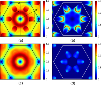
Figure 1: (Color online) Intensity maps of the $1/S$ spin wave spectrum for the $S=1/2$ triangular-lattice antiferromagnet with easy$-$plane anisotropy $\alpha=1$ (upper row) and $\alpha=0.95$ (lower row). (a) and (c), renormalized magnon energy $\bar{\varepsilon}_{\mathbf{k}}$. (b) and (d), magnon decay rate $\Gamma_{\mathbf{k}}$. $\Gamma=(0,0)$, $\Sigma=(2\pi/3,0)$, $X=(\pi,0)$, $K=(4\pi/3,0)$, $M=(0,2\pi/\sqrt{3})$, and $Y=(0,\pi/\sqrt{3})$ points in (a) are highlighted. Note, the overall damping of spin waves is strongly reduced and the decay region shrinks with increasing anisotropy. The realistic magnon decays disappear at $\alpha\approx 0.92$ Chernyshev and Zhitomirsky (2009).

Inelastic neutron scattering data of a TLAF reveals well$-$defined sharp modes in the low$-$energy excitation spectrum accompanied with a broad continuum at intermediate and high energies Coldea et al. (2003); Zhou et al. (2012); Oh et al. (2013). A number of competing theoretical proposals, ranging from a proximate spin$-$liquid phase Kohno et al. (2007); Ghioldi et al. (2015) to enhanced magnon$-$magnon interactions Veillette et al. (2005); Dalidovich et al. (2006); Mourigal et al. (2013) have been proposed to explain the nature of the spin wave excitation spectrum. Our starting point is the spin $S$, nearest$-$neighbor $XXZ$ antiferromagnetic model on the triangular lattice. The spin$-$wave theory Hamiltonian in the local $(x-z)$ rotating frame associated with the ordering wave vector $\mathbf{Q}=(4\pi/3,0)$, $K-$ point in BZ, takes the following form Chernyshev and Zhitomirsky (2009):

$$\mathcal{H}= J\sum_{\langle ij\rangle}[\alpha S_{i}^{y}S_{j}^{y}+\cos(\theta_{i}-\theta_{j})(S_{i}^{z}S_{j}^{z}+S_{i}^{x}S_{j}^{x})$$ (1)

$$+\sin(\theta_{i}-\theta_{j})(S_{i}^{z}S_{j}^{x}-S_{i}^{x}S_{j}^{z})].$$

where $\theta_{i}=\mathbf{Q}\cdot\mathbf{r}_{i}$ and we have also introduced an easy$-$plane anisotropy parameter $\alpha\in[0,1]$. In Appendix A we outline the derivation of the effective interacting spin$-$wave Hamiltonian $\mathcal{H}_{\mathrm{eff}}$ in the first order $1/S$ expansion with respect to linear spin$-$wave theory. The resulting expression is

$$\mathcal{H}_{\mathrm{eff}}= \sum_{\mathbf{k}}(\varepsilon_{\mathbf{k}}+\delta\varepsilon_{\mathbf{k}})b_{\mathbf{k}}^{\dagger}b_{\mathbf{k}}+\frac{1}{2!}\sum_{\{\mathbf{k}_{i}\}}V_{a}(b_{1}^{\dagger}b_{2}^{\dagger}b_{3}+\mathrm{H.c.})$$ (2)

$$+\frac{1}{3!}\sum_{\{\mathbf{k}_{i}\}}V_{b}(b_{1}^{\dagger}b_{2}^{\dagger}b_{3}^{\dagger}+\mathrm{H.c.})+\sum_{\{\mathbf{k}_{i}\}}V_{c}b_{1}^{\dagger}b_{2}^{\dagger}b_{3}b_{4},$$

where we have adopted the convention that $1=\mathbf{k}_{1}$, $2=\mathbf{k}_{2}$, etc, and momentum conservation is assumed for various $\mathbf{k}$-summations. The bare magnon dispersion given by the linear spin$-$wave theory is expressed as

$$\varepsilon_{\mathbf{k}}=3JS\sqrt{(1-\gamma_{\mathbf{k}})(1+2\alpha\gamma_{\mathbf{k}})},$$ (3)

with $\gamma_{\mathbf{k}}=\frac{1}{3}[\cos k_{x}+2\cos(k_{x}/2)\cos(\sqrt{3}k_{y}/2)]$. The explicit forms for the interacting vertices $\delta\varepsilon$, $V_{a,b}$, and $V_{c}$ are detailed in Appendix A. At zero temperature the bare magnon propagator is defined as

$$\mathrm{G}_{0}^{-1}(\mathbf{k},\omega)=\omega-\varepsilon_{\mathbf{k}}+i0^{+}.$$ (4)

The first order $1/S$ correction to the magnon energy is determined by the Dyson equation

$$\omega-\varepsilon_{\mathbf{k}}-\Sigma(\mathbf{k},\omega)=0,$$ (5)

with the one-loop self-erengy $\Sigma(\mathbf{k},\omega)=\Sigma_{a}(\mathbf{k},\omega)+\Sigma_{b}(\mathbf{k},\omega)+\Sigma_{c}(\mathbf{k})$, where $\Sigma_{c}(\mathbf{k})=\delta\varepsilon_{\mathbf{k}}$ is a frequency-independent Hartree-Fock correction, while $\Sigma_{a,b}(\mathbf{k},\omega)$ are calculated as Chubukov et al. (1994); Chernyshev and Zhitomirsky (2006); Starykh et al. (2006); Chernyshev and Zhitomirsky (2009)

$$\Sigma_{a}(\mathbf{k},\omega) = \frac{1}{2}\sum_{\mathbf{p}}\frac{|V_{a}(\mathbf{p},\mathbf{k}-\mathbf{p};\mathbf{k})|^{2}}{\omega-\varepsilon_{\mathbf{p}}-\varepsilon_{\mathbf{k}-\mathbf{p}}+i0^{+}},$$ (6)

$$\Sigma_{b}(\mathbf{k},\omega) = -\frac{1}{2}\sum_{\mathbf{p}}\frac{|V_{b}(\mathbf{p},-\mathbf{k}-\mathbf{p},\mathbf{k})|^{2}}{\omega+\varepsilon_{\mathbf{p}}+\varepsilon_{\mathbf{k}+\mathbf{p}}-i0^{+}}.$$ (7)

The on-shell solution consists of setting $\omega=\varepsilon_{\mathbf{k}}$ in the self-energy (6) and (7) leads to the following expression for the $1/S$ renormalized spectrum

$$\omega_{\mathbf{k}}\equiv\bar{\omega}_{\mathbf{k}}-i\Gamma_{\mathbf{k}}=\varepsilon_{\mathbf{k}}+\Sigma(\mathbf{k},\varepsilon_{\mathbf{k}}).$$ (8)

In Fig. 1 we display the intensity maps for the renormalization of magnon energy $\bar{\varepsilon}_{\mathbf{k}}$ and the magnon decay rate $\Gamma_{\mathbf{k}}$ for the $S=1/2$ triangular antiferromagnet for $\alpha=1$ (isotropic) and $\alpha=0.95$ (anisotropic) case. From Fig. 1(d) we observe that the magnon decay rate decreases drastically in the presence of anisotropy. This is due to the reduced phase volume where the kinematic constraint $\varepsilon_{\mathbf{k}}=\varepsilon_{\mathbf{p}}-\varepsilon_{\mathbf{k}-\mathbf{p}}$ in the self-energy (6) is satisfied. The magnon decay intensity maps Fig. 1(b) and Fig. 1(d) play an important role in understanding the origins of the multipeak RIXS structure shown in Fig. 6 and Fig. 7.

III Indirect RIXS Correlator

In Mott insulating systems, multimagnon excitations can be created dynamically by the presence of the core-hole potential in the intermediate state of indirect RIXS process. The effective scattering operator, in the first order, under the assumption of the ultra-short core-hole life-time (UCL) expansion is given by van den Brink (2007); Forte et al. (2008)

$$\mathcal{R}_{\mathbf{q}}=J\sum_{i,\boldsymbol{\delta}}e^{i\mathbf{q}\cdot\mathbf{r}_{i}}\mathbf{S}_{i}\cdot\mathbf{S}_{i+\boldsymbol{\delta}},$$ (9)

where $\mathbf{r}_{i}$ is the position of the ion absorbing the incident photon and $\boldsymbol{\delta}$ denotes the neighboring vectors. After consecutive Holstein-Primakoff and Bogoliubov transformations, the magnon creation parts of the RIXS scattering operator can be expressed in terms of the bosonic operators as

$$\mathcal{R}_{\mathbf{q}}=\sum_{1+2=\mathbf{q}}M(1,2)b_{1}^{\dagger}b_{2}^{\dagger}+\sum_{1+2+3=\mathbf{q}}N(1,2,3)b_{1}^{\dagger}b_{2}^{\dagger}b_{3}^{\dagger},$$ (10)

with the bimagnon scattering matrix element expression is given by

$$M(1,2)= \frac{3JS}{2!}\Big{\{}[1+\gamma_{\mathbf{q}}+(\alpha-\frac{1}{2})(\gamma_{1}+\gamma_{2})](u_{1}v_{2}+v_{1}u_{2})$$ (11)

$$-(\alpha+\frac{1}{2})(\gamma_{1}+\gamma_{2})(u_{1}u_{2}+v_{1}v_{2})\Big{\}},$$

and the trimagnon scattering matrix element is given by

$$N(1,2,3)= \frac{3JS}{3!}i\sqrt{\frac{3}{2S}}\big{[}(\bar{\gamma}_{1}-\bar{\gamma}_{2+3}-\frac{1}{4}\bar{\gamma}_{\mathbf{q}})(u_{1}+v_{1})$$ (12)

$$\times(u_{2}v_{3}+v_{2}u_{3})+(\bar{\gamma}_{2}-\bar{\gamma}_{1+3}-\frac{1}{4}\bar{\gamma}_{\mathbf{q}})(u_{2}+v_{2})$$

$$\times(u_{1}v_{3}+v_{1}u_{3})+(\bar{\gamma}_{3}-\bar{\gamma}_{1+2}-\frac{1}{4}\bar{\gamma}_{\mathbf{q}})(u_{3}+v_{3})$$

$$\times(u_{1}v_{2}+v_{1}u_{2})\big{]},$$

where $u$, $v$ and $\bar{\gamma}$ are defined in Appendix A. The three-boson term in our theory has no analog in the collinear phases of a square lattice quantum magnet. Note, the corrections from magnon interactions for the trimagnon intensity appear at the $1/S^{2}$ order and are neglected in the remainder of this paper.

The frequency- and momentum-dependent magnetic scattering intensity is related to multimagnon response function via the fluctuation-dissipation theorem. The full $1/S$ corrections to the indirect RIXS susceptibility is the sum of bimagnon and trimagnon contributions given by

$$I(\mathbf{q},\omega) = -\frac{1}{\pi}\mathrm{Im}[\chi_{2}(\mathbf{q},\omega)+\chi_{3}(\mathbf{q},\omega)],$$ (13)

$$= -\frac{1}{\pi}\mathrm{Im}[\chi_{\mathrm{RIXS}}(\mathbf{q},\omega)],$$

which involve an interacting two$-$magnon susceptibility $\chi_{2}(\mathbf{q},\omega)$ and a non$-$interacting three$-$magnon susceptibility $\chi_{3}(\mathbf{q},\omega)$. The susceptibilities can be expressed explicitly from the corresponding multi-magnon Green’s function defined as

$$\chi_{2}(\mathbf{q},\omega) = \sum_{\mathbf{k}\mathbf{k}^{\prime}}M_{\mathbf{k}}M_{\mathbf{k}^{\prime}}\Pi_{\mathbf{k}\mathbf{k}^{\prime}}(\mathbf{q},\omega),$$ (14)

$$\chi_{3}(\mathbf{q},\omega) = \sum_{\mathbf{k}\mathbf{p};\mathbf{k}^{\prime}\mathbf{p}^{\prime}}N_{\mathbf{k},\mathbf{p}}N_{\mathbf{k}^{\prime},\mathbf{p}^{\prime}}\Lambda_{\mathbf{k}\mathbf{p};\mathbf{k}^{\prime}\mathbf{p}^{\prime}}(\mathbf{q},\omega),$$ (15)

where $\Pi$ and $\Lambda$ are denoted as the bimagnon and trimagnon propagators, respectively. The momentum-dependent two-magnon and three-magnon Green’s function in terms of Bogoliubov quasiparticles are defined as

$$i\Pi_{\mathbf{k}\mathbf{k}^{\prime}}(\mathbf{q},t) = \langle\mathcal{T}b_{\mathbf{k}+\mathbf{q}}(t)b_{-\mathbf{k}}(t)b_{\mathbf{k}^{\prime}+\mathbf{q}}^{\dagger}b_{-\mathbf{k}^{\prime}}^{\dagger}\rangle,$$ (16)

$$i\Lambda_{\mathbf{k}\mathbf{p};\mathbf{k}^{\prime}\mathbf{p}^{\prime}}(\mathbf{q},t) = \langle\mathcal{T}b_{\mathbf{k}}(t)b_{\mathbf{q}-\mathbf{k}-\mathbf{p}}(t)b_{\mathbf{p}}(t)b_{\mathbf{k}^{\prime}}^{\dagger}b_{\mathbf{q}-\mathbf{k}^{\prime}-\mathbf{p}^{\prime}}^{\dagger}b_{\mathbf{p}^{\prime}}^{\dagger}\rangle,$$ (17)

where $\mathcal{T}$ is the time-ordering operator and $\langle\cdot\rangle$ is the average of the ground state. In the following sections, using Eq. (16) and Eq. (17), we will compute the noninteracting and the interacting RIXS spectra.

IV RESULTS AND DISCUSSION

IV.1 Noninteracting bi$-$ and trimagnon spectra

Using Eqs. (11)$-$(12) and applying Wick’s theorem to Eq. (16) and Eq. (17), we obtain the following expressions for the noninteracting bimagnon ($I_{2}(\mathbf{q},\omega)$) and trimagnon ($I_{3}(\mathbf{q},\omega)$) scattering intensity

$$I_{2}(\mathbf{q},\omega) = 2\sum_{\mathbf{k}}M_{\mathbf{k}+\mathbf{q},-\mathbf{k}}^{2}\delta(\omega-\varepsilon_{\mathbf{k}+\mathbf{q}}-\varepsilon_{\mathbf{k}}),$$ (18)

$$I_{3}(\mathbf{q},\omega) = 6\sum_{\mathbf{k},\mathbf{p}}N_{\mathbf{k},\mathbf{q}-\mathbf{k}-\mathbf{p},\mathbf{p}}^{2}\delta(\omega-\varepsilon_{\mathbf{k}}-\varepsilon_{\mathbf{q}-\mathbf{k}-\mathbf{p}}-\varepsilon_{\mathbf{p}}).$$ (19)

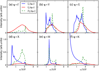
Figure 2: (Color online) Non-interacting bimagnon ($I_{2}(\mathbf{q},\omega)$) and trimagnon ($I_{3}(\mathbf{q},\omega)$) RIXS intensity of the isotropic TLAF at momentum transfer wavevector $\mathbf{q}$ corresponding to the special high symmetry points of a triangular lattice magnetic BZ. The bimagnon DOS $D_{2}(\mathbf{q},\omega)$ is also shown as a dashed line. The nonzero intensity at the $\Gamma$ and at the $K$ point is a unique RIXS feature of the noncollinear ground state configuration.

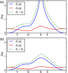
Figure 3: (Color online) The non-interacting bimagnon and trimagnon total spectral weight for the anisotropic TLAF with (a) $\alpha=1$ and (b) $\alpha=0.95$. Irrespective of the presence of anisotropy, the bimagnon and trimagnon intensity complement each other at the zone center and at the zone boundary. Introduction of anisotropy removes the singularity due to the opening up of a gap in the spin wave spectrum.

In Fig. 2, we show the results for the $S=1/2$ isotropic Heisenberg model at various points in the BZ. At the $\Gamma$ point the contribution is purely from the trimagnon excitations, see Fig. 2(a). The bimagnon RIXS intensity displays a nonzero elastic peak at the $K$ point, see Fig. 2(f). The indirect RIXS spectra even at the noninteracting level, in a noncollinear quantum magnet, exhibits significant differences from the collinear ordered quantum magnets where the intensity vanishes at the BZ center and at the antiferromagnetic wavevectorvan den Brink (2007); Nagao and Igarashi (2007); Forte et al. (2008); Luo et al. (2014).

Figure 4: (Color online) Pure trimagnon contribution to the RIXS intensity. (a) no anisotropy ($\alpha$=1) (b) with anisotropy ($\alpha$=0.95).

The noninteracting bimagnon RIXS intensity in Eq. 18 is proportional to the bare two$-$magnon density of states (DOS)

$$D_{2}(\mathbf{q},\omega)=\sum_{\mathbf{k}}\delta(\omega-\varepsilon_{\mathbf{k}+\mathbf{q}}-\varepsilon_{\mathbf{k}}),$$ (20)

A close inspection on the DOS in Fig. 2 shows that these Van-Hove singularities which originate from the maximum or saddle points of the two-magnon continuum $\varepsilon_{\mathbf{k}+\mathbf{q}}+\varepsilon_{\mathbf{k}}$ partially transfer to the RIXS intensity, see Fig.2(b$-$e), and the spectrum line shape at $\mathbf{q}=M$ (Fig.2(e)) resembles the DOS with minimal RIXS matrix element effects.

In Fig. 3 we show the variation of the total spectral weight across the BZ for the bimagnon and trimagnon component, respectively. By using the bare intensity Eqs. (18) and Eqs. (19) we obtain

$$\mathcal{S}_{2}(\mathbf{q}) = \int_{0}^{\infty}\mathrm{d}\omega I_{2}(\mathbf{q},\omega)=2\sum_{\mathbf{k}}M^{2}(\mathbf{k}+\mathbf{q},-\mathbf{k}),$$ (21)

$$\mathcal{S}_{3}(\mathbf{q}) = \int_{0}^{\infty}\mathrm{d}\omega I_{3}(\mathbf{q},\omega)=6\sum_{\mathbf{k}}N^{2}(\mathbf{k},\mathbf{q}-\mathbf{k}-\mathbf{p};\mathbf{p}),$$ (22)

In general, the trimagnon excitation dominates the indirect RIXS total spectral weight in the vicinity of the BZ center, while the bimagnon spectral weight becomes overwhelmingly large at the boundary of the BZ where the three-magnon intensity is negligible. The most remarkable feature of the isotropic model, see Fig. 3(a), is the elastic peak at the antiferromagnetic wave vector which resembles the longitudinal dynamic structure factor probed by neutron-scattering experiments Canali and Wallin (1993); Lorenzana et al. (2005); Mourigal et al. (2013). Upon inclusion of anisotropy, $\alpha=0.95$, the elastic peak at $\mathbf{q}=K$ disappears, see Fig. 3(b), since a gap is now introduced in the spin$-$wave dispersion (4) at the ordering wave vector.

In Fig. 4 we show the pure trimagnon contribution along the $\Gamma\rightarrow M$ path obtained using the noninteracting three$-$magnon susceptibility $\chi_{3}(\mathbf{q},\omega)$ in Eq. (15). We plot the spectra both in the presence and in the absence of anisotropy. We observe that the trimagnon spectra peak occurs at a higher energy approximately around $6JS$ around the $\Gamma$ point, which downshifts before undergoing an upward shift to $6JS$ around the M point. In the presence of anisotropy, see Fig. 4(b), there is an overall upward shift of the energy peak. The observed effect could be an artifact of considering a noninteracting trimagnon spectra. In the next section we consider the interacting bimagnon RIXS intensity up to 1/S order.

IV.2 Bimagnon excitations: $1/S$ corrections

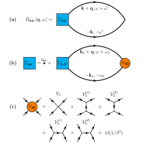
Figure 5: (Color online) Diagrammatic representation for (a) two-magnon propagator $\Pi_{\mathbf{k}\mathbf{k}^{\prime}}(\mathbf{q},\omega)$, (b) Bethe-Salpeter euqation of the vertex function $\Gamma_{\mathbf{k}\mathbf{k}^{\prime}}(\omega,\omega^{\prime})$ and (c) the $1/S$ order irreducible interaction $\mathcal{V}_{\mathrm{IR}}$. Solid lines with an arrow in (a) and (b) stand for the single-magnon propagators.

We now proceed with the analysis of $1/S$ correction to the two-magnon Green’s function by taking into account both the self-energy correction to the single magnon propagator $G$ according to the Dyson equation and the vertex insertions to the two-magnon propagator $\Pi$ which satisfies the Bethe-Salpeter (BS) equation Davies et al. (1971); Canali and Girvin (1992). The diagrammatic representation of such procedure is depicted in Fig. 5(a) and  5(b). The total irreducible bimagnon scattering vertices in Fig. 5(c) fall into two categories, which we term as direct ($\mathcal{V}_{4}$) and indirect ($\mathcal{V}^{a-d}_{3}$).

The direct collision between the two main magnons is caused by the quartic vertex $\mathcal{V}_{4}$ while the cubic vertices $\mathcal{V}^{a-d}_{3}$ represent the indirect magnon$-$magnon interactions. Note that in the direct ladder interaction events the two main magnons created in the RIXS process are stable while virtual decays and recombination are allowed in the indirect collision process. Using Feynman rules in momentum space then yields the following equations for the two$-$particle propagator and the vertex function

$$\Pi_{\mathbf{k}\mathbf{k}^{\prime}}(\mathbf{q},\omega)= 2i\int\frac{\mathrm{d}\omega^{\prime}}{2\pi}\mathrm{G}_{\mathbf{k}+\mathbf{q}}(\omega+\omega^{\prime})\mathrm{G}_{-\mathbf{k}}(-\omega^{\prime})\Gamma_{\mathbf{k}\mathbf{k}^{\prime}}(\omega,\omega^{\prime}),$$ (23)

$$\Gamma_{\mathbf{k}\mathbf{k}^{\prime}}(\omega,\omega^{\prime})= \delta_{\mathbf{k}\mathbf{k}^{\prime}}+\sum_{\mathbf{k}_{1}}2i\int\frac{\mathrm{d}\omega_{1}}{2\pi}\mathrm{G}_{\mathbf{k}_{1}+\mathbf{q}}(\omega+\omega_{1})\mathrm{G}_{-\mathbf{k}_{1}}(-\omega_{1})$$

$$\times\mathcal{V}^{\mathrm{IR}}_{\mathbf{k}\mathbf{k}_{1}}(\omega^{\prime},\omega_{1})\Gamma_{\mathbf{k}_{1}\mathbf{k}^{\prime}}(\omega,\omega_{1}),$$ (24)

with the basic one-magnon propagator up to $1/S$ order defined as

$$\mathrm{G}^{-1}(\mathbf{k},\omega) = \omega-\omega_{\mathbf{k}}+i0^{+}.$$ (25)

The factor of $2$ in Eq.(23) and Eq.(IV.2) stem from the two sets of contributions differing by the interchange of dummy momenta $\mathbf{k}(\mathbf{k}_{1})+\mathbf{q}$ and $-\mathbf{k}(\mathbf{k}_{1})$ according to the Wick’s theorem. The lowest order two-particle irreducible interaction vertex $\mathcal{V}_{\mathrm{IR}}$, shown in Fig. 5(c), reads as

$$\mathcal{V}_{\mathrm{IR}}=\mathcal{V}_{4}+\mathcal{V}_{3}^{(a)}+\mathcal{V}_{3}^{(b)}+\mathcal{V}_{3}^{(c)}+\mathcal{V}_{3}^{(d)},$$ (26)

where the frequency-independent four-point vertex $\mathcal{V}_{4}$ coming from the quartic Hamiltonian has the form

$$\mathcal{V}_{4}=V_{c}(\mathbf{k}_{1}+\mathbf{q},-\mathbf{k}_{1};\mathbf{k}+\mathbf{q},-\mathbf{k}),$$ (27)

and the other four vertices $\mathcal{V}_{3}^{(a-d)}$ in the same $1/S$ order which are assembled from two three-point vertices and one frequency-dependent propagator can be written as

$$\mathcal{V}_{3}^{(a)}= \frac{1}{(2!)^{2}}[V_{a}(\mathbf{k}_{1}+\mathbf{q},\mathbf{k}-\mathbf{k}_{1};\mathbf{k}+\mathbf{q})\mathrm{G}_{0}(\mathbf{k}-\mathbf{k}_{1},\omega^{\prime}-\omega_{1})$$ (28)

$$\times V^{\ast}_{a}(-\mathbf{k},\mathbf{k}-\mathbf{k}_{1};-\mathbf{k}_{1})],$$

$$\mathcal{V}_{3}^{(b)}= \frac{1}{(2!)^{2}}[V^{\ast}_{a}(\mathbf{k}+\mathbf{q},\mathbf{k}_{1}-\mathbf{k};\mathbf{k}_{1}+\mathbf{q})\mathrm{G}_{0}(\mathbf{k}_{1}-\mathbf{k},\omega_{1}-\omega^{\prime})$$ (29)

$$\times V_{a}(-\mathbf{k}_{1},\mathbf{k}_{1}-\mathbf{k};-\mathbf{k})],$$

$$\mathcal{V}_{3}^{(c)}= \frac{1}{(2!)^{2}}[V_{a}(\mathbf{k}_{1}+\mathbf{q},-\mathbf{k}_{1};\mathbf{q})\mathrm{G}_{0}(\mathbf{q},\omega)$$ (30)

$$\times V^{\ast}_{a}(\mathbf{k}+\mathbf{q},-\mathbf{k};\mathbf{q})],$$

$$\mathcal{V}_{3}^{(d)}= \frac{1}{(3!)^{2}}[V_{b}(\mathbf{k}_{1}+\mathbf{q},-\mathbf{k}_{1},\mathbf{q})\mathrm{G}_{0}(-\mathbf{q},-\omega)$$ (31)

$$\times V^{\ast}_{b}(\mathbf{k}+\mathbf{q},-\mathbf{k},\mathbf{q})],$$

where we have retained only the bare propagator $\mathrm{G}_{0}$ for each intermediate line in $\mathcal{V}_{3}^{(a-d)}$ in the spirit of $1/S$ expansion. We further assume that two on-shell magnons are created and annihilated in the repeated ladder scattering process with $\omega^{\prime}\approx-\varepsilon^{(0)}_{\mathbf{k}}$ and $\omega_{1}\approx-\varepsilon^{(0)}_{\mathbf{k}_{1}}$ Perkins and Brenig (2008); Perkins et al. (2013). This approximation is best for sharp spectral peaks of the two main magnons in the scattering process where all the lowest order irreducible vertices are not explicitly frequency dependent. Based on the above simplifications, we now derive the final solution of the interacting RIXS intensity from the ladder approximation BS equation.

An approach to solving the coupled BS equations is to decompose the irreducible vertices into lattice harmonics as demonstrated for the case of collinear antiferromagnet Nagao and Igarashi (2007); Luo et al. (2014). An inspection of the interaction vertices for the TLAF reveals that $\mathcal{V}_{3}^{(a,b)}$ can not be separated into finite sum of products of the triangular-lattice harmonics, thus Eq.(14) can not be algebraically solved in terms of a finite number of scattering channels. However, a numerical solution can be performed on finite lattices by summing over $N$ points of $\mathbf{k}$ in the 1^st BZ, leading to a $N\times N$ system for the linear solver. We adopt this numerical approach to compute the interacting intensity plots.

We begin with substituting (23) and (IV.2) into (14),

$$\chi_{2}=\sum_{\mathbf{k}\mathbf{k}^{\prime}}M_{\mathbf{k}}M_{\mathbf{k}^{\prime}}\Big{[}\delta_{\mathbf{k}\mathbf{k}^{\prime}}\Pi_{\mathbf{k}}+\Pi_{\mathbf{k}}\sum_{\mathbf{k}_{1}}V_{\mathbf{k}\mathbf{k}_{1}}\Pi_{\mathbf{k}_{1}\mathbf{k}^{\prime}}\Big{]},$$ (32)

where $\Pi_{\mathbf{k}}=2[\omega-\varepsilon_{\mathbf{k}+\mathbf{q}}-\varepsilon_{\mathbf{k}}+i0^{+}]^{-1}$ represents the renormalizated two-magnon propagator in the absence of vertex correction. The BZ on finite lattices can be divided into $\sqrt{N}\times\sqrt{N}$ meshes with the replacement of the continuous momenta $(\mathbf{k},\mathbf{k}^{\prime},\mathbf{k}_{1})$ to discrete variables $(\mathrm{m,n,l})$. The elements for the bimagnon susceptibility matrix are given by

$$\mathrm{\hat{\chi}}_{\mathrm{mn}}=M_{\mathrm{m}}M_{\mathrm{n}}\Big{[}\delta_{\mathrm{mn}}\Pi_{\mathrm{m}}+\Pi_{\mathrm{m}}\sum_{\mathrm{l}}V_{\mathrm{ml}}\Pi_{\mathrm{ln}}\Big{]}.$$ (33)

We then obtain the eigenvalue equation for these discrete momenta

$$\mathcal{A}_{\mathrm{mn}} = \mathcal{G}_{\mathrm{mn}}+\sum_{\mathrm{l}}\Gamma_{\mathrm{ml}}\mathcal{A}_{\mathrm{ln}},$$ (34)

where the new functions are defined as

$$\mathcal{A}_{\mathrm{mn}}=\hat{\Pi}_{\mathrm{mn}}M_{\mathrm{n}},~{}\mathcal{G}_{\mathrm{mn}}=\delta_{\mathrm{mn}}\Pi_{\mathrm{m}}M_{\mathrm{n}},~{}\Gamma_{\mathrm{ml}}=\Pi_{\mathrm{m}}V_{\mathrm{ml}}.$$ (35)

A direct solution to (34) gives the final form of the $\mathrm{\hat{\chi}}$ matrix as

$$\mathrm{\hat{\chi}}=\mathcal{\hat{D}}\textbf{[}\mathbf{\hat{1}}-\hat{\Gamma}\textbf{]}^{-1}\mathcal{\hat{G}},$$ (36)

where all the matrices in Eq. (36) have $N\times N$ dimensions with the matrix elements explicitly defined as

$$\mathbf{\hat{1}}_{\mathrm{mn}} = \delta_{\mathrm{mn}},\mathcal{\hat{D}}_{\mathrm{mn}}=\delta_{\mathrm{mn}}M_{\mathrm{m}},$$ (37)

$$\hat{\Gamma}_{\mathrm{mn}} = \Pi_{\mathrm{m}}V_{\mathrm{mn}},~{}\mathcal{\hat{G}}_{\mathrm{mn}}=\delta_{\mathrm{mn}}\Pi_{\mathrm{m}}M_{\mathrm{n}}.$$ (38)

The interacting pure bimagnon RIXS susceptibility can then be computed as

$$\mathrm{\chi}_{2}(\mathbf{q},\omega)=\sum_{\mathrm{m,n}}\mathrm{\hat{\chi}}_{\mathrm{mn}}.$$ (39)

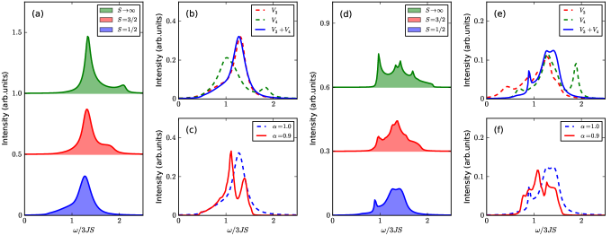
Figure 6: (Color online) Interacting bimagnon RIXS intensity for transformed momenta $\mathbf{q}=M$ (a-c) and $\mathbf{q}=Y$ (d-f). In (a) and (d) the evolution of the interacting bimagnon intensity profile with increasing spin value $S$ for the isotropic model is shown. In (a) and (d): $S\rightarrow\infty$ (top frame), $S=3/2$ (middle frame), and $S=1/2$ (bottom frame). In (b) and (e) comparison of the contribution from the direct ($\mathcal{V}_{4}$), indirect ($\mathcal{V}_{3}$) and full ($\mathcal{V}_{3}+\mathcal{V}_{4}$) vertices correction to the RIXS spectrum for $S=1/2$ and $\alpha=1$ are displayed. In (c) and (f) the effects of easy-plane anisotropy on the splitting feature of the interacting bimagnon spectrum are shown.

In Fig. 6 we plot the results for interacting bimagnon RIXS intensity. We choose two special BZ momenta values, $M$ and $Y$, to illustrate our findings. In Fig. 6(a) and Fig. 6(d) we show the progression of the indirect RIXS spectra shape as the spin $S$ value is changed from the classical case $S\rightarrow\infty$ (top), to $S=3/2$ (middle), to the maximal quantum case of $S=1/2$ (bottom). While the classical RIXS spectra from both momenta contain peaks due to the presence of Van Hove singularities, introduction of quantum fluctuations cause some of these spurious peaks to disappear. But observe that in the S = $1/2$ case the spectra shape is strikingly different. In the absence of anisotropy at the $\mathbf{q}=M$ (roton transfer momentum), we observe a single peak at an energy of $4JS$. However, at the $\mathbf{q}=Y$ point there is a multipeak structure, see Fig. 6(d). Now comparing with the magnon decay intensity map, Fig. 1(b), it is evident that there is a direct correlation between the stability of the spin wave modes and the appearance of a single or multipeak structure. The above mentioned comparison is not restricted to these two choosen points. Comparision of the RIXS spectra generated from other special high symmetry momentum transfer also have the same features, see Fig. 7. Based on these observations we propose that RIXS can be used as a probe to detect the presence of the roton mode in a TLAF. Furthermore, to provide a comprehensive picture of the effects of geometrical frustration and anisotropy we introduce a small anisotropy $\alpha=0.9$ in the system. From Fig. 6(c) and Fig. 6(f) it is clear that inclusion of anisotropy causes further peak splitting. Thus a proper explanation of the RIXS spectra features in a TLAF involves analyzing both the effects of magnon damping and anisotropy.

The $\mathcal{V}_{4}$ and $\mathcal{V}_{3}$ vertices play an important role in the generation of the RIXS bimagnon spectra. Especially at the roton point it is worth noting that including only the direct collision vertex does not renormalize the single$-$peak structure in the extreme quantum condition with $S=1/2$, Fig. 6(b). The major contribution to the interacting RIXS spectra originates from the indirect vertices arising from the three-magnon interaction terms. This indicates that renormalization of the spectra is due to the indirect $\mathcal{V}_{3}$ vertices which involve virtual decay and recombination of the two main magnons in the scattering process. This is different from the $\mathbf{q}=Y$ point where both the $\mathcal{V}_{4}$ and $\mathcal{V}_{3}$ vertices contribute, as seen in Fig. 6(e).

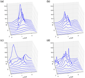
Figure 7: (Color online) Full indirect RIXS spectra $I_{2}+I_{3}$ of the $S=1/2$ $XXZ$ triangular$-$lattice antiferromagnet with $\alpha=1$; (a) and (c) and $\alpha=0.9$; (b) and (d), along the high symmetry path $\Gamma\rightarrow M$ and $\Gamma\rightarrow K$ in the BZ.

Before we end this section it is important to point out an important difference between a Raman scattering calculation and RIXS. In the case of RIXS, the contributions of diagrams $\mathcal{V}_{3}^{(c)}$ and $\mathcal{V}_{3}^{(d)}$ vanish identically when the transferred momenta belongs to the $\Gamma-M$ path or related symmetrical lines in the BZ in accordance with the magnetic Raman scattering study for which $\mathbf{q}=0$ Perkins and Brenig (2008). To demonstrate this fact we consider the contributions of the two$-$particle irreducible vertices $\mathcal{V}_{3}^{(c)}$ and $\mathcal{V}_{3}^{(d)}$ which are already in separated forms as functions of $\mathbf{k}$ and $\mathbf{k}^{\prime}$. The corresponding reducible vertex function Eq. (IV.2) with respect to these diagrams can be directly obtained as

$$\Gamma_{\mathbf{k}\mathbf{k}^{\prime}}= \delta_{\mathbf{k}\mathbf{k}^{\prime}}+V^{\ast}_{a(b)}(\mathbf{k})f(\mathbf{q},\omega),$$ (40)

where $f(\mathbf{q},\omega)$ is a function of $\omega$ and $\mathbf{q}$ only. Barring the noninteracting contributions the vertex correction to the RIXS susceptibility is given by

$$\chi_{V}(\mathbf{q},\omega) =f(\mathbf{q},\omega)\sum_{\mathbf{k}^{\prime}}M_{\mathbf{k}^{\prime}}\sum_{\mathbf{k}}M_{\mathbf{k}}\Pi_{\mathbf{k}}V^{\ast}_{a(b)}(\mathbf{k})$$

$$=\mathrm{const}\times\sum_{\mathbf{k}}M_{\mathbf{k}}\Pi_{\mathbf{k}}V^{\ast}_{a(b)}(\mathbf{k}).$$ (41)

In the above both $M_{\mathbf{k}}$ and $\Pi_{\mathbf{k}}$ are even functions of $\mathbf{k}$, while the function $V^{\ast}_{a(b)}(\mathbf{k})=V^{\ast}_{a(b)}(\mathbf{k}+\mathbf{q},-\mathbf{k},\mathbf{q})$ are odd functions with respect to $\mathbf{k}$ when momentum $\mathbf{q}$ is along the $\Gamma M$ line (e.g. $q_{x}=0$). Thus, by virtue of the $C_{3}$ symmetry of hexagonal lattices we can conclude that the total contributions of diagrams $\mathcal{V}_{3}^{(c)}$ and $\mathcal{V}_{3}^{(d)}$ vanish identically when transformed momenta $\mathbf{q}$ are located in the lines from the center of the BZ to the middle of the BZ boundary. This implies that the source processes are prohibited in the repeated ladder scattering events when transferred momenta are along these symmetrical paths.

IV.3 Total RIXS intensity

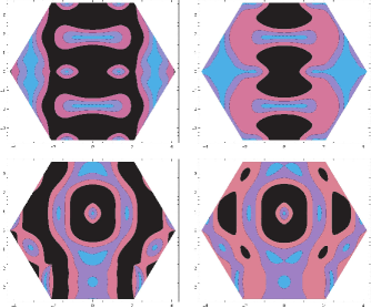
Figure 8: (Color online) Contour plot of the bimagnon velocity in the first BZ of TLAF for transferred momenta $\mathbf{q}=M$ (first row) and $\mathbf{q}=Y$ (second row) with $\alpha=1$ and $\alpha=0.9$. First column is the bimagnon velocity in the absence of anisotropy. Second column is for the anisotropic ($\alpha=0.9$) case. Lowest velocity contours indicated by blue (grey) bands. Relative higher velocities indicated by black regions.

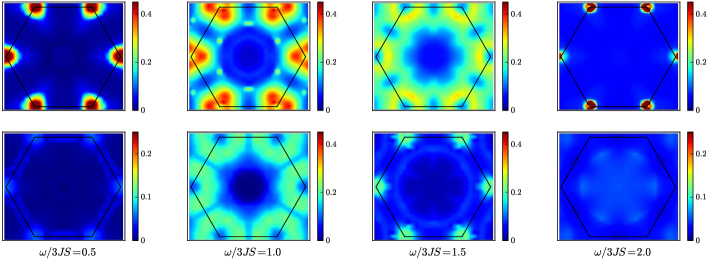
Figure 9: (Color online) Intensity plots of the constant-$\omega$ scans of the full RIXS intensity $I(\mathbf{q},\omega)$ scaled by $(3JS)^{2}$ for the $S=1/2$ $XXZ$ triangular lattice antiferromagnet in the $\mathbf{q}$ plane with $\alpha=1$ (upper) and $\alpha=0.9$ (lower) at four representative energies. The prominent peaks on the corners are strongly reduced in the presence of anisotropy in qualitative agreement with the noninteracting total spectral weight.

Using Eq. (13) we compute the full indirect RIXS spectra. In Fig. 7 we display the RIXS line plots along the $\Gamma\rightarrow M$ path and along the $\Gamma\rightarrow K$ path, respectively. The features observed are reminiscent of those discussed for the noninteracting trimagnon spectra and the full interacting bimagnon spectra. As noted earlier, we find that at the $\Gamma$ point the spectra originates purely from the trimagnon contribution, irrespective of the presence or absence of anisotropy. However, inclusion of anisotropy causes a downshift of the bimagnon contribution and an upward shift of the trimagnon spectra. Anisotropy gives rise to further splitting in the bimagnon case, however, the trimagnon spectra is not affected. The occurence of peak splitting observed in the RIXS spectrum can be predicted by observing the bimagnon velocity plot. In a previous publication on the square lattice Heisenberg magnet Luo et al. (2014) we had highlighted the connection between bimagnon velocity and the appearance of multipeak structure in the RIXS spectra. Interestingly enough, even within the context of a TLAF this relationship persists. To demonstrate this correlation, in Fig. 8, we show the bimagnon velocity intensity plot in both the presence and absence of anisotropy for the $\mathbf{q}=M$ and the $\mathbf{q}=Y$ point. The black regions represent the highest moving bimagnon velocities which clearly disappear with the inclusion of anistropy. As more puddles of slow moving bimagnon velocity appears, so does the appearance of a multipeak structure as shown in Fig. 7. At the $\mathbf{q}=M$ point the single roton peak melts away with increasing anistropy which comes along with low bimagnon velocity. A similar effect is observed at the $\mathbf{q}=Y$ point, where with increasing anisotropy there are greater pockets of slow moving bimagnon. Hence, with anisotropy the peak splits further at $Y$ point. Finally, in Fig. 9 we present the expected constant$-\omega$ scans of the total interacting RIXS intensity for four selected energies from low energy to a high energy. One of the advantages of these constant$-$energy scans, which is reminiscent of the INS experiments, is that prominent peak structures are easy to distinguish Mourigal et al. (2013). For the isotropic model the interacting RIXS intensity is strongly peaked on the corners of the hexagonal BZ at low and high energies, while these peaks disperse along the edges of the BZ at intermediate energies. However the presence of $XXZ$ anisotropic strongly reduces these prominent features, which is in qualitative agreement with the noninteracting total spectral weight shown in Fig. 2.

V Conclusion

At present, there exists no theoretical guidance for experimentalists on how to analyze and interpret the RIXS spectra of an ordered phase in a geometrically frustrated quantum magnet. Although a proposal for detecting spin$-$chirality terms in triangular lattice Mott insulators via RIXS has been put forward Ko and Lee (2011), there has been no analysis on the effect of geometrical frustration and anisotropy on the indirect RIXS spectra. In this paper, using a $1/S$ expansion spin$-$wave theory involving Bethe$-$Salpeter corrections we investigate the key signatures of noncollinear ground state ordering in the indirect RIXS spectrum of a TLAF. We conclude that in the absence of anisotropy the root cause of the multipeak structure is magnon decay. This mechanism is different from that of a square lattice where strong frustrating further neighbor interactions and anisotropy are required to cause peak splitting (instability). In the introduction we had put forward a couple of questions$-$ (a) How does the presence of an intrinsic damping affect the indirect K$-$edge RIXS spectra? and (b) What role does the interplay between geometrical frustration and spin anisotropy have on the RIXS spectra? Based on our calculations, we conclude that magnon damping does affect the spectra, causing the RIXS peak to be either stable (no splitting) or unstable (splitting leading to multipeak) in the absence or presence of damping, respectively. Geometrical frustration introduces noncollinear ordering which introduces magnon damping. The stability or instability of the ensuing magnon mode then dictates the appearance of a single or multipeak structure. By comparing the K$-$edge RIXS intensity of the square lattice case, to that of the TLAF, we find that the RIXS intensity does not vanish at the $\Gamma$ point and at the antiferromagnetic wavevector. At the $\Gamma$ point, the bimagnon intensity is zero and the single peak spectra results purely from the trimagnon contribution, approximately at energy scale of $6JS$ corresponding to the three magnon energy. This provides experimentalists with a means to detect purely trimagnon RIXS spectra at the K$-$edge. Our proposed scheme of detecting trimagnon excitations is different from that put forward in the paper by Ament and Brink Ament and van den Brink , since we are not considering the L$-$edge. The single roton peak occurs at an energy of $4JS$ and can be used as an experimental signature to detect roton modes in a TLAF. In conclusion, our theoretical investigation demonstrates that RIXS has the potential to probe and provide a comprehensive characterization of the microscopic properties of bimagnon and trimagnon excitations in the TLAF across the entire BZ, which is beyond the capabilities of traditional low$-$energy optical techniques Devereaux and Hackl (2007); Vernay et al. (2007); Perkins and Brenig (2008); Perkins et al. (2013).

Appendix A Derivation of interacting spin-wave theory

We utilize the Holstein-Primakoff transformation to bosonize the local rotating Hamiltonian (1)

$$S_{i}^{z}=S-a_{i}^{\dagger}a_{i},\ S_{i}^{-}=a^{\dagger}\sqrt{2S-a_{i}^{\dagger}a_{i}},\ S_{i}^{+}=(S_{i}^{-})^{\dagger},$$ (42)

with subsequent expansion of square root to first order in $a_{i}^{\dagger}a_{i}/2S$. This is followed by a Fourier transformation. The Fourier transformed Hamiltonian takes the form

$$\mathcal{H}=H_{0}+H_{2}+H_{3}+H_{4}+O(S^{-1}).$$ (43)

The first term corresponds to the classical energy and the quadratic Hamiltonian reads

$$H_{2}=\sum_{\mathbf{k}}\Big{[}A_{\mathbf{k}}a_{\mathbf{k}}^{\dagger}a_{\mathbf{k}}+\frac{1}{2}B_{\mathbf{k}}(a_{\mathbf{k}}^{\dagger}a_{-\mathbf{k}}^{\dagger}+a_{-\mathbf{k}}a_{\mathbf{k}})\Big{]},$$

$$A_{\mathbf{k}}=3JS[1+(\alpha-\frac{1}{2})\gamma_{\mathbf{k}}],\ B_{\mathbf{k}}=-3JS(\alpha+\frac{1}{2})\gamma_{\mathbf{k}},$$ (44)

with the structure factor $\gamma_{\mathbf{k}}$ defined as

$$\gamma_{\mathbf{k}}=\frac{1}{3}\Big{(}\cos k_{x}+2\cos\frac{k_{x}}{2}\cos\frac{\sqrt{3}}{2}k_{y}\Big{)}.$$ (45)

We then diagonalize the harmonic part $H_{2}$ by the Bogoliubov transformation

$$a_{\mathbf{k}}=u_{\mathbf{k}}b_{\mathbf{k}}+v_{\mathbf{k}}b_{-\mathbf{k}}^{\dagger},$$ (46)

with the parameters $u_{\mathbf{k}}$ and $v_{\mathbf{k}}$ defined as

$$u_{\mathbf{k}}^{2},v_{\mathbf{k}}^{2}=\frac{A_{\mathbf{k}}\pm\varepsilon_{\mathbf{k}}}{2\varepsilon_{\mathbf{k}}},u_{\mathbf{k}}v_{\mathbf{k}}=-\frac{B_{\mathbf{k}}}{2\varepsilon_{\mathbf{k}}},$$ (47)

and the linear spin-wave theory dispersion given by

$$\varepsilon_{\mathbf{k}}=\sqrt{A_{\mathbf{k}}^{2}-B_{\mathbf{k}}^{2}}=3JS\epsilon_{\mathbf{k}},$$ (48)

where we have defined the dimensionless energy

$$\epsilon_{\mathbf{k}}=\sqrt{(1-\gamma_{\mathbf{k}})(1+2\gamma_{\mathbf{k}})}.$$ (49)

Performing the Bogoliubov transformations in the cubic interaction term $H_{3}$ we obtain

$$H_{3}= \frac{1}{2!}\sum_{\mathbf{k}_{1}+\mathbf{k}_{2}=\mathbf{k}_{3}}V_{a}(\mathbf{k}_{1},\mathbf{k}_{2};\mathbf{k}_{3})(b_{\mathbf{k}_{1}}^{\dagger}b_{\mathbf{k}_{2}}^{\dagger}b_{\mathbf{k}_{3}}+\mathrm{H.c.})$$ (50)

$$+\frac{1}{3!}\sum_{\mathbf{k}_{1}+\mathbf{k}_{2}+\mathbf{k}_{3}=0}V_{b}(\mathbf{k}_{1},\mathbf{k}_{2},\mathbf{k}_{3})(b_{\mathbf{k}_{1}}^{\dagger}b_{\mathbf{k}_{2}}^{\dagger}b_{\mathbf{k}_{3}}^{\dagger}+\mathrm{H.c.})$$

The explicit forms for the three-boson interaction vertices are

$$V_{a}(1,2;3)= 3Ji\sqrt{\frac{3S}{2}}\big{[}\bar{\gamma}_{1}(u_{1}+v_{1})(u_{2}u_{3}+v_{2}v_{3})+\bar{\gamma}_{2}(u_{2}+v_{2})$$ (51)

$$\times(u_{1}u_{3}+v_{1}v_{3})-\bar{\gamma}_{3}(u_{3}+v_{3})(u_{1}v_{2}+v_{1}u_{2})\big{]},$$

$$V_{b}(1,2,3)= 3Ji\sqrt{\frac{3S}{2}}\big{[}\bar{\gamma}_{1}(u_{1}+v_{1})(u_{2}v_{3}+v_{2}u_{3})+\bar{\gamma}_{2}(u_{2}+v_{2})$$ (52)

$$\times(u_{1}v_{3}+v_{1}u_{3})+\bar{\gamma}_{3}(u_{3}+v_{3})(u_{1}v_{2}+v_{1}u_{2})\big{]},$$

where $u_{i}$, $v_{i}$ are Bogoliubov parameters and the function $\bar{\gamma}_{\mathbf{k}}$ is defined as

$$\bar{\gamma}_{\mathbf{k}}= \frac{1}{3}\Big{(}\sin k_{x}-2\sin\frac{k_{x}}{2}\cos\frac{\sqrt{3}}{2}k_{y}\Big{)}.$$ (53)

The three-boson vertex $V_{a}$ and $V_{b}$ in $H_{3}$ describes interaction between one- and two-magnon states and are called the decay and the source vertex, respectively.

To derive the explicit forms of the quartic interaction term $H_{4}$, it is convenient to introduce the following Hartree-Fock averages

$$n = \langle a_{i}^{\dagger}a_{i}\rangle=\frac{1}{2}c_{0}+\frac{2\alpha-1}{4}c_{1}-\frac{1}{2},$$ (54)

$$m = \langle a_{i}^{\dagger}a_{j}\rangle=\frac{1}{2}c_{1}+\frac{2\alpha-1}{4}c_{2},$$ (55)

$$\Delta = \langle a_{i}a_{j}\rangle=\frac{2\alpha+1}{4}c_{2},$$ (56)

$$\delta = \langle a_{i}^{2}\rangle=\frac{2\alpha+1}{4}c_{1},$$ (57)

with the two-dimensional integrals

$$c_{l}=\sum_{\mathbf{k}}\frac{(\gamma_{\mathbf{k}})^{l}}{\epsilon_{\mathbf{k}}},\ (l=0,1,2).$$ (58)

After the mean-field decoupling, the quartic part is decomposed as

$$H_{4}=\delta H_{0}+\delta H_{2}+\tilde{H}_{4}.$$ (59)

The first term $\delta H_{0}$ is the correction to the ground-state energy and the quadratic parts reads

$$\delta H_{2}=\sum_{\mathbf{k}}\Big{[}\delta A_{\mathbf{k}}a_{\mathbf{k}}^{\dagger}a_{\mathbf{k}}+\frac{1}{2}\delta B_{\mathbf{k}}(a_{\mathbf{k}}^{\dagger}a_{-\mathbf{k}}^{\dagger}+a_{-\mathbf{k}}a_{\mathbf{k}})\Big{]},$$ (60)

with

$$\delta A_{\mathbf{k}}= \frac{3}{2}[(1+2\alpha)\Delta+(1-2\alpha)m-2n]$$

$$+\frac{3}{4}[(1+2\alpha)\delta+2(1-2\alpha)n-4m]\gamma_{\mathbf{k}},$$

$$\delta B_{\mathbf{k}}= \frac{3}{4}[(1+2\alpha)m+(1-2\alpha)\Delta]$$ (61)

$$+\frac{3}{4}[(1-2\alpha)\delta+2(+2\alpha)n-4\Delta]\gamma_{\mathbf{k}}.$$

We then obtain the Hartree-Fock correction to the harmonic spin-wave spectrum

$$\delta\varepsilon_{\mathbf{k}}=(u_{\mathbf{k}}^{2}+v_{\mathbf{k}}^{2})\delta A_{\mathbf{k}}+2u_{\mathbf{k}}v_{\mathbf{k}}\delta B_{\mathbf{k}}.$$ (62)

The normal-ordered term $\tilde{H}_{4}$ describes the multi-particle interactions. Here we only display the explicit expression for the lowest order irreducible two-particle scattering amplitude which is relevant for the our calculations as

$$\tilde{H}_{4}^{2-p}=\sum_{\mathbf{k}_{1}+\mathbf{k}_{2}=\mathbf{k}_{3}+\mathbf{k}_{4}}V_{c}(\mathbf{k}_{1},\mathbf{k}_{2};\mathbf{k}_{3},\mathbf{k}_{4})b_{\mathbf{k}_{1}}^{\dagger}b_{\mathbf{k}_{2}}^{\dagger}b_{\mathbf{k}_{3}}b_{\mathbf{k}_{4}},$$ (63)

with the vertex function

$$V_{c}(1,2;3,4)= \frac{3JS}{16S}\Big{\{}(2\alpha+1)(\gamma_{1}+\gamma_{2}+\gamma_{4})(u_{1}u_{2}u_{3}v_{4}+v_{1}v_{2}v_{3}u_{4})+(2\alpha+1)(\gamma_{1}+\gamma_{2}+\gamma_{3})(u_{1}u_{2}v_{3}u_{4}+v_{1}v_{2}u_{3}v_{4})$$ (64)

$$+(2\alpha+1)(\gamma_{2}+\gamma_{3}+\gamma_{4})(u_{1}v_{2}u_{3}u_{4}+v_{1}u_{2}v_{3}v_{4})+(2\alpha+1)(\gamma_{1}+\gamma_{3}+\gamma_{4})(u_{1}v_{2}v_{3}v_{4}+v_{1}u_{2}u_{3}u_{4})$$

$$-[2(\gamma_{1-3}+\gamma_{2-3}+\gamma_{1-4}+\gamma_{2-4})+(2\alpha-1)(\gamma_{1}+\gamma_{2}+\gamma_{3}+\gamma_{4})](u_{1}u_{2}u_{3}u_{4}+v_{1}v_{2}v_{3}v_{4})$$

$$-[2(\gamma_{1+2}+\gamma_{3+4}+\gamma_{1-3}+\gamma_{2-4})+(2\alpha-1)(\gamma_{1}+\gamma_{2}+\gamma_{3}+\gamma_{4})](u_{1}v_{2}u_{3}v_{4}+v_{1}u_{2}v_{3}u_{4})$$

$$-[2(\gamma_{1+2}+\gamma_{3+4}+\gamma_{1-4}+\gamma_{2-3})+(2\alpha-1)(\gamma_{1}+\gamma_{2}+\gamma_{3}+\gamma_{4})](u_{1}v_{2}v_{3}u_{4}+v_{1}u_{2}u_{3}v_{4})\Big{\}}.$$

By collecting all these terms together, we finally obtain the effective interacting spin$-$wave Hamiltonian Eq. (2).

Appendix B Exact versus numerical solution to the BS equation

Table 1: Definition of the channels $v_{\mathrm{n}}(\mathbf{k})$

$n$	$v_{n}(\mathbf{k})$	$n$	$v_{n}(\mathbf{k})$
1	$u_{\mathbf{k}+\mathbf{q}}u_{\mathbf{k}}$	15	$u_{\mathbf{k}+\mathbf{q}}v_{\mathbf{k}}\cos k_{x}\cos\frac{\sqrt{3}}{2}k_{y}$
2	$v_{\mathbf{k}+\mathbf{q}}v_{\mathbf{k}}$	16	$v_{\mathbf{k}+\mathbf{q}}u_{\mathbf{k}}\cos k_{x}\cos\frac{\sqrt{3}}{2}k_{y}$
3	$u_{\mathbf{k}+\mathbf{q}}v_{\mathbf{k}}$	17	$u_{\mathbf{k}+\mathbf{q}}u_{\mathbf{k}}\sin k_{x}\sin\frac{\sqrt{3}}{2}k_{y}$
4	$v_{\mathbf{k}+\mathbf{q}}u_{\mathbf{k}}$	18	$v_{\mathbf{k}+\mathbf{q}}v_{\mathbf{k}}\sin k_{x}\sin\frac{\sqrt{3}}{2}k_{y}$
5	$u_{\mathbf{k}+\mathbf{q}}u_{\mathbf{k}}\cos k_{x}$	19	$u_{\mathbf{k}+\mathbf{q}}v_{\mathbf{k}}\sin k_{x}\sin\frac{\sqrt{3}}{2}k_{y}$
6	$v_{\mathbf{k}+\mathbf{q}}v_{\mathbf{k}}\cos k_{x}$	20	$v_{\mathbf{k}+\mathbf{q}}u_{\mathbf{k}}\sin k_{x}\sin\frac{\sqrt{3}}{2}k_{y}$
7	$u_{\mathbf{k}+\mathbf{q}}v_{\mathbf{k}}\cos k_{x}$	21	$u_{\mathbf{k}+\mathbf{q}}u_{\mathbf{k}}\cos k_{x}\sin\frac{\sqrt{3}}{2}k_{y}$
8	$v_{\mathbf{k}+\mathbf{q}}u_{\mathbf{k}}\cos k_{x}$	22	$v_{\mathbf{k}+\mathbf{q}}v_{\mathbf{k}}\cos k_{x}\sin\frac{\sqrt{3}}{2}k_{y}$
9	$u_{\mathbf{k}+\mathbf{q}}u_{\mathbf{k}}\sin k_{x}$	24	$u_{\mathbf{k}+\mathbf{q}}v_{\mathbf{k}}\cos k_{x}\sin\frac{\sqrt{3}}{2}k_{y}$
10	$v_{\mathbf{k}+\mathbf{q}}v_{\mathbf{k}}\sin k_{x}$	24	$v_{\mathbf{k}+\mathbf{q}}u_{\mathbf{k}}\cos k_{x}\sin\frac{\sqrt{3}}{2}k_{y}$
11	$u_{\mathbf{k}+\mathbf{q}}v_{\mathbf{k}}\sin k_{x}$	25	$u_{\mathbf{k}+\mathbf{q}}u_{\mathbf{k}}\sin k_{x}\cos\frac{\sqrt{3}}{2}k_{y}$
12	$v_{\mathbf{k}+\mathbf{q}}u_{\mathbf{k}}\sin k_{x}$	26	$v_{\mathbf{k}+\mathbf{q}}v_{\mathbf{k}}\sin k_{x}\cos\frac{\sqrt{3}}{2}k_{y}$
13	$u_{\mathbf{k}+\mathbf{q}}u_{\mathbf{k}}\cos k_{x}\cos\frac{\sqrt{3}}{2}k_{y}$	27	$u_{\mathbf{k}+\mathbf{q}}v_{\mathbf{k}}\sin k_{x}\cos\frac{\sqrt{3}}{2}k_{y}$
14	$v_{\mathbf{k}+\mathbf{q}}v_{\mathbf{k}}\cos k_{x}\cos\frac{\sqrt{3}}{2}k_{y}$	28	$v_{\mathbf{k}+\mathbf{q}}u_{\mathbf{k}}\sin k_{x}\cos\frac{\sqrt{3}}{2}k_{y}$

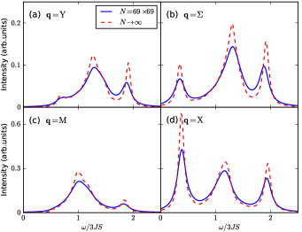
Figure 10: (Color online) Interacting bimagnon RIXS intensity renormalized only by the direct interaction vertex ($\mathcal{V}_{4}$) based on the exact ($N\rightarrow\infty$) versus numerical ($N=69\times 69$) solution of the Bethe-Salpeter equation for a $S=1/2$ isotropic triangular lattice antiferromagnet at various momenta in the BZ.

To test the validity of our numerical method on finite lattices ($N=69\times 69$), we adopt the exact solution approach to solving a BS equation outlined in Appendix B of our publication Ref. [Luo et al., 2014]. We obtain a separated form for the four-point vertex $\mathcal{V}_{4}$ for the Heisenberg model ($\alpha=1$) on triangular lattice which has the following expression

$$\mathcal{V}_{4}(\mathbf{k}_{1}+\mathbf{q},-\mathbf{k}_{1};\mathbf{k}+\mathbf{q},-\mathbf{k})=\sum_{\mathrm{m,n}=1}^{\mathrm{28}}v_{\mathrm{m}}(\mathbf{k})\hat{\Gamma}_{\mathrm{mn}}v_{\mathrm{n}}(\mathbf{k}_{1}).$$ (65)

The channels $v_{\mathrm{n}}(\mathbf{k})$ are defined in Table 1 with the matrix elements of $\hat{\Gamma}$ denoted by

$$\hat{\Gamma}=\frac{3JS}{16S}\left(\begin{array}[]{cccc}\hat{S}_{1}&\hat{T}\\ \hat{T}&\hat{S}_{2}\\ \end{array}\right),$$ (66)

where the blocks are given by

$$\hat{T}=\left(\begin{array}[]{cccccccccccccc}2&2\lambda&-\frac{2}{3}\phi&-\frac{2}{3}\phi&0&0&0&0&0&0&0&0&0&1\\ 2\lambda&2&-\frac{2}{3}\phi&-\frac{2}{3}\phi&0&0&0&0&0&0&0&0&0&2\\ -\frac{2}{3}\chi&0&2\chi&2\chi&0&0&0&0&0&0&0&0&-\frac{8}{3}\chi&0\\ 0&-\frac{2}{3}\chi&2\chi&2\chi&0&0&0&0&0&0&0&0&0&-\frac{8}{3}\chi\\ 0&2\chi&-\frac{2}{3}\chi&-\frac{2}{3}\chi&0&0&0&0&0&0&0&0&0&0\\ 2\chi&0&-\frac{2}{3}\chi&-\frac{2}{3}\chi&0&0&0&0&0&0&0&0&0&0\\ \frac{2}{3}\mu&0&-2\mu&-2\mu&0&0&0&0&0&0&0&0&\frac{8}{3}\mu&0\\ 0&\frac{2}{3}\mu&-2\mu&-2\mu&0&0&0&0&0&0&0&0&0&\frac{8}{3}\mu\\ 0&-2\mu&\frac{2}{3}\mu&\frac{2}{3}\mu&0&0&0&0&0&0&0&0&0&0\\ -2\mu&0&\frac{2}{3}\mu&\frac{2}{3}\mu&0&0&0&0&0&0&0&0&0&0\\ \frac{2}{3}\nu&0&-2\nu&-2\nu&0&0&0&0&0&0&0&0&\frac{8}{3}\nu&0\\ 0&\frac{2}{3}\nu&-2\nu&-2\nu&0&0&0&0&0&0&0&0&0&\frac{8}{3}\nu\\ 0&-2\nu&\frac{2}{3}\nu&\frac{2}{3}\nu&0&0&0&0&0&0&0&0&0&0\\ -2\nu&0&\frac{2}{3}\nu&\frac{2}{3}\nu&0&0&0&0&0&0&0&0&0&0\\ \end{array}\right),$$

$$\hat{S}_{1}=\left(\begin{array}[]{cccccccccccccc}0&0&0&0&-\frac{1}{3}\theta&0&1&C^{0}_{q}&\frac{1}{3}S^{0}_{q}&0&0&-S^{0}_{q}&-\frac{2}{3}\phi&0\\ &0&0&0&0&-\frac{1}{3}\theta&C^{0}_{q}&1&0&\frac{1}{3}S^{0}_{q}&-S^{0}_{q}&0&0&-\frac{2}{3}\phi\\ &&-\frac{4}{3}\gamma_{\mathbf{q}}&-4\gamma_{\mathbf{q}}&\theta&\theta&-\frac{1}{3}\theta&-\frac{1}{3}\theta&-S^{0}_{q}&-S^{0}_{q}&\frac{1}{3}S^{0}_{q}&\frac{1}{3}S^{0}_{q}&2\phi&2\phi\\ &&&-\frac{4}{3}\gamma_{\mathbf{q}}&\theta&\theta&-\frac{1}{3}\theta&-\frac{1}{3}\theta&-S^{0}_{q}&-S^{0}_{q}&\frac{1}{3}S^{0}_{q}&\frac{1}{3}S^{0}_{q}&2\phi&2\phi\\ &&&&-\frac{1}{3}\theta&0&0&0&\frac{4}{3}S^{0}_{q}&0&0&0&0&0\\ &&&&&-\frac{1}{3}\theta&0&0&0&\frac{4}{3}S^{0}_{q}&0&0&0&0\\ &&&&&&-\frac{4}{3}&0&0&0&0&\frac{4}{3}S^{0}_{q}&0&0\\ &&&&&&&-\frac{4}{3}&0&0&-\frac{4}{3}&0&0&0\\ &&&&&&&&-\frac{1}{3}\vartheta&0&0&0&0&0\\ &&&&&&&&&-\frac{1}{3}\vartheta&0&0&0&0\\ &&&&&&&&&&-\frac{4}{3}&\frac{4}{3}C^{0}_{q}&0&0\\ &&&&&&&&&&&-\frac{4}{3}&0&0\\ &&&&&&&&&&&&-\frac{8}{3}\phi&0\\ &&&&&&&&&&&&&-\frac{8}{3}\phi\\ \end{array}\right),$$

$$\hat{S}_{2}=\left(\begin{array}[]{cccccccccccccc}-\frac{8}{3}&-\frac{8}{3}\lambda&0&0&0&-\frac{8}{3}\chi&0&0&0&\frac{8}{3}\lambda&0&0&0&\frac{8}{3}\nu\\ &-\frac{8}{3}&0&0&-\frac{8}{3}\chi&0&0&0&\frac{8}{3}\mu&0&0&0&\frac{8}{3}\nu&0\\ &&-\frac{8}{3}\theta&0&0&0&-\frac{8}{3}\nu&0&0&0&-\frac{8}{3}\mu&0&0&0\\ &&&-\frac{8}{3}\theta&0&0&0&-\frac{8}{3}\nu&0&0&0&-\frac{8}{3}\mu&0&0\\ &&&&-\frac{8}{3}&-\frac{8}{3}\lambda&0&0&0&-\frac{8}{3}\nu&0&-\frac{8}{3}\mu&0&0\\ &&&&&-\frac{8}{3}&0&0&-\frac{8}{3}\nu&0&0&0&-\frac{8}{3}\mu&0\\ &&&&&&\frac{8}{3}\varphi&0&0&0&-\frac{8}{3}\chi&0&0&0\\ &&&&&&&\frac{8}{3}\varphi&0&0&0&-\frac{8}{3}\chi&0&0\\ &&&&&&&&-\frac{8}{3}&-\frac{8}{3}\lambda&0&0&0&-\frac{8}{3}\chi\\ &&&&&&&&&-\frac{8}{3}&0&0&-\frac{8}{3}\chi&0\\ &&&&&&&&&&\frac{8}{3}\varphi&0&0&0\\ &&&&&&&&&&&\frac{8}{3}\varphi&0&0\\ &&&&&&&&&&&&-\frac{8}{3}&\frac{8}{3}\lambda\\ &&&&&&&&&&&&&-\frac{8}{3}\\ \end{array}\right).$$

In the above we have introduced the following notations:

$$C^{0}_{q} = \cos q_{x},\ C^{1}_{q}=\cos\frac{q_{x}}{2},\ C^{2}_{q}=\cos\frac{\sqrt{3}}{2}q_{y},$$ (67)

$$S^{0}_{q} = \cos q_{x},\ S^{1}_{q}=\cos\frac{q_{x}}{2},\ S^{2}_{q}=\cos\frac{\sqrt{3}}{2}q_{y},$$ (68)

$$\lambda = C^{1}_{q}C^{2}_{q},\ \mu=C^{1}_{q}S^{2}_{q},\ \nu=S^{1}_{q}C^{2}_{q},\ \chi=S^{1}_{q}S^{2}_{q},$$ (69)

$$\theta = C^{0}_{q}+1,\ \vartheta=C^{0}_{q}-1,$$ (70)

$$\phi = C^{1}_{q}C^{2}_{q}+1,\ \varphi=C^{1}_{q}C^{2}_{q}-1.$$ (71)

Only the upper right parts of $\hat{S}_{1}$ and $\hat{S}_{2}$ are shown since the matrices are symmetrical.

In Fig. 10 we show the results of our computation for $S=1/2$ and $\alpha=1$. The numerical solution of Eq. (39) by considering only the $\mathcal{V}_{4}$ vertex is performed with $69\times 69$ lattice sites, while the integrals arising in the exact solution are solved on a mesh of size $252\times 252$ and then extrapolated to $N\rightarrow\infty$  Luo et al. (2014).

References

- Anderson (1973) P. W. Anderson, “Resonating valence bonds: A new kind of insulator?” Mater. Res. Bull. 8, 153 (1973).
- Jolicoeur and Le Guillou (1989) Th. Jolicoeur and J. C. Le Guillou, “Spin-wave results for the triangular heisenberg antiferromagnet,” Phys. Rev. B 40, 2727–2729 (1989).
- Miyake (1992) Satoru J. Miyake, “Spin-wave results for the staggered magnetization of triangular heisenberg antiferromagnet,” J. Phys. Soc. Jpn. 61, 983–988 (1992).
- Chubukov et al. (1994) A V Chubukov, S Sachdev, and T Senthil, “Large-s expansion for quantum antiferromagnets on a triangular lattice,” J. Phys.: Condens. Matter 6, 8891 (1994).
- Capriotti et al. (1999) Luca Capriotti, Adolfo E. Trumper, and Sandro Sorella, “Long-range néel order in the triangular heisenberg model,” Phys. Rev. Lett. 82, 3899–3902 (1999).
- Zheng et al. (2006a) Weihong Zheng, John O. Fjærestad, Rajiv R. P. Singh, Ross H. McKenzie, and Radu Coldea, “Excitation spectra of the spin- triangular-lattice heisenberg antiferromagnet,” Phys. Rev. B 74, 224420 (2006a).
- White and Chernyshev (2007) Steven R. White and A. L. Chernyshev, “Neél order in square and triangular lattice heisenberg models,” Phys. Rev. Lett. 99, 127004 (2007).
- Li et al. (2015) P. H. Y. Li, R. F. Bishop, and C. E. Campbell, “Quasiclassical magnetic order and its loss in a spin- heisenberg antiferromagnet on a triangular lattice with competing bonds,” Phys. Rev. B 91, 014426 (2015).
- Huse and Elser (1988) David A. Huse and Veit Elser, “Simple variational wave functions for two-dimensional heisenberg spin-½ antiferromagnets,” Phys. Rev. Lett. 60, 2531–2534 (1988).
- Bernu et al. (1994) B. Bernu, P. Lecheminant, C. Lhuillier, and L. Pierre, “Exact spectra, spin susceptibilities, and order parameter of the quantum heisenberg antiferromagnet on the triangular lattice,” Phys. Rev. B 50, 10048–10062 (1994).
- Singh and Huse (1992) Rajiv R. P. Singh and David A. Huse, “Three-sublattice order in triangular- and kagomé-lattice spin-half antiferromagnets,” Phys. Rev. Lett. 68, 1766–1769 (1992).
- Shirata et al. (2012) Yutaka Shirata, Hidekazu Tanaka, Akira Matsuo, and Koichi Kindo, “Experimental realization of a spin- triangular-lattice heisenberg antiferromagnet,” Phys. Rev. Lett. 108, 057205 (2012).
- Koutroulakis et al. (2015) G. Koutroulakis, T. Zhou, Y. Kamiya, J. D. Thompson, H. D. Zhou, C. D. Batista, and S. E. Brown, “Quantum phase diagram of the triangular-lattice antiferromagnet ,” Phys. Rev. B 91, 024410 (2015).
- Susuki et al. (2013) Takuya Susuki, Nobuyuki Kurita, Takuya Tanaka, Hiroyuki Nojiri, Akira Matsuo, Koichi Kindo, and Hidekazu Tanaka, “Magnetization process and collective excitations in the triangular-lattice heisenberg antiferromagnet ,” Phys. Rev. Lett. 110, 267201 (2013).
- Ono et al. (2003) T. Ono, H. Tanaka, H. Aruga Katori, F. Ishikawa, H. Mitamura, and T. Goto, “Magnetization plateau in the frustrated quantum spin system ,” Phys. Rev. B 67, 104431 (2003).
- Kadowaki et al. (1987) Hiroaki Kadowaki, Koji Ubukoshi, Kinshiro Hirakawa, José L. Martínez, and Gen Shirane, “Experimental study of new type phase transition in triangular lattice antiferromagnet vcl2,” J. Phys. Soc. Jpn 56, 4027–4039 (1987).
- Ishii et al. (2011) R. Ishii, S. Tanaka, K. Onuma, Y. Nambu, M. Tokunaga, T. Sakakibara, N. Kawashima, Y. Maeno, C. Broholm, D. P. Gautreaux, J. Y. Chan, and S. Nakatsuji, “Successive phase transitions and phase diagrams for the quasi-two-dimensional easy-axis triangular antiferromagnet rb 4 mn(moo 4 ) 3,” Eur. Phys. Lett. 94, 17001 (2011).
- Poienar et al. (2010) M. Poienar, F. Damay, C. Martin, J. Robert, and S. Petit, “Spin dynamics in the geometrically frustrated multiferroic ,” Phys. Rev. B 81, 104411 (2010).
- Toth et al. (2011) S. Toth, B. Lake, S. A. J. Kimber, O. Pieper, M. Reehuis, A. T. M. N. Islam, O. Zaharko, C. Ritter, A. H. Hill, H. Ryll, K. Kiefer, D. N. Argyriou, and A. J. Williams, “120∘ helical magnetic order in the distorted triangular antiferromagnet ,” Phys. Rev. B 84, 054452 (2011).
- Toth et al. (2012) S. Toth, B. Lake, K. Hradil, T. Guidi, K. C. Rule, M. B. Stone, and A. T. M. N. Islam, “Magnetic soft modes in the distorted triangular antiferromagnet ,” Phys. Rev. Lett. 109, 127203 (2012).
- Coldea et al. (2001a) R. Coldea, D. A. Tennant, A. M. Tsvelik, and Z. Tylczynski, “Experimental realization of a 2d fractional quantum spin liquid,” Phys. Rev. Lett. 86, 1335–1338 (2001a).
- Chen et al. (2013) Ru Chen, Hyejin Ju, Hong-Chen Jiang, Oleg A. Starykh, and Leon Balents, “Ground states of spin- triangular antiferromagnets in a magnetic field,” Phys. Rev. B 87, 165123 (2013).
- Schmidt and Thalmeier (2014) Burkhard Schmidt and Peter Thalmeier, “Quantum fluctuations in anisotropic triangular lattices with ferromagnetic and antiferromagnetic exchange,” Phys. Rev. B 89, 184402 (2014).
- Hauke et al. (2011) Philipp Hauke, Tommaso Roscilde, Valentin Murg, J Ignacio Cirac, and Roman Schmied, “Modified spin-wave theory with ordering vector optimization: spatially anisotropic triangular lattice and j 1 j 2 j 3 model with heisenberg interactions,” New Journal of Physics 13, 075017 (2011).
- Kohno et al. (2007) Masanori Kohno, Oleg A. Starykh, and Leon Balents, “Spinons and triplons in spatially anisotropic frustrated antiferromagnets,” Nature Phys. 3, 790 (2007).
- Swanson et al. (2009) M. Swanson, J. T. Haraldsen, and R. S. Fishman, “Critical anisotropies of a geometrically frustrated triangular-lattice antiferromagnet,” Phys. Rev. B 79, 184413 (2009).
- Fishman and Okamoto (2010) Randy S. Fishman and Satoshi Okamoto, “Noncollinear magnetic phases of a triangular-lattice antiferromagnet and of doped ,” Phys. Rev. B 81, 020402 (2010).
- Ghioldi et al. (2015) E. A. Ghioldi, A. Mezio, L. O. Manuel, R. R. P. Singh, J. Oitmaa, and A. E. Trumper, “Magnons and excitation continuum in xxz triangular antiferromagnetic model: Application to ,” Phys. Rev. B 91, 134423 (2015).
- Suzuki et al. (2014) Nobuo Suzuki, Fumitaka Matsubara, Sumiyoshi Fujiki, and Takayuki Shirakura, “Absence of classical long-range order in an heisenberg antiferromagnet on a triangular lattice,” Phys. Rev. B 90, 184414 (2014).
- Weichselbaum and White (2011) Andreas Weichselbaum and Steven R. White, “Incommensurate correlations in the anisotropic triangular heisenberg lattice,” Phys. Rev. B 84, 245130 (2011).
- Hauke (2013) Philipp Hauke, “Quantum disorder in the spatially completely anisotropic triangular lattice,” Phys. Rev. B 87, 014415 (2013).
- Coldea et al. (2001b) R. Coldea, S. M. Hayden, G. Aeppli, T. G. Perring, C. D. Frost, T. E. Mason, S.-W. Cheong, and Z. Fisk, “Spin waves and electronic interactions in ,” Phys. Rev. Lett. 86, 5377–5380 (2001b).
- Rønnow et al. (2001) H. M. Rønnow, D. F. McMorrow, R. Coldea, A. Harrison, I. D. Youngson, T. G. Perring, G. Aeppli, O. Syljuåsen, K. Lefmann, and C. Rischel, “Spin dynamics of the 2d spin quantum antiferromagnet copper deuteroformate tetradeuterate (cftd),” Phys. Rev. Lett. 87, 037202 (2001).
- Ament et al. (2011) Luuk J. P. Ament, Michel van Veenendaal, Thomas P. Devereaux, John P. Hill, and Jeroen van den Brink, “Resonant inelastic x-ray scattering studies of elementary excitations,” Rev. Mod. Phys. 83, 705–767 (2011).
- Hill et al. (2008) J. P. Hill, G. Blumberg, Young-June Kim, D. S. Ellis, S. Wakimoto, R. J. Birgeneau, Seiki Komiya, Yoichi Ando, B. Liang, R. L. Greene, D. Casa, and T. Gog, “Observation of a 500 mev collective mode in and using resonant inelastic x-ray scattering,” Phys. Rev. Lett. 100, 097001 (2008).
- Ellis et al. (2010) D. S. Ellis, Jungho Kim, J. P. Hill, S. Wakimoto, R. J. Birgeneau, Y. Shvyd’ko, D. Casa, T. Gog, K. Ishii, K. Ikeuchi, A. Paramekanti, and Young-June Kim, “Magnetic nature of the 500 mev peak in observed with resonant inelastic x-ray scattering at the -edge,” Phys. Rev. B 81, 085124 (2010).
- van den Brink (2007) J. van den Brink, “The theory of indirect resonant inelastic x-ray scattering on magnons,” Europhys. Lett. 80, 47003 (2007).
- Nagao and Igarashi (2007) Tatsuya Nagao and Jun-Ichi Igarashi, “Two-magnon excitations in resonant inelastic x-ray scattering from quantum heisenberg antiferromagnets,” Phys. Rev. B 75, 214414 (2007).
- Forte et al. (2008) Filomena Forte, Luuk J. P. Ament, and Jeroen van den Brink, “Magnetic excitations in probed by indirect resonant inelastic x-ray scattering,” Phys. Rev. B 77, 134428 (2008).
- Luo et al. (2014) Cheng Luo, Trinanjan Datta, and Dao Xin Yao, “Spectrum splitting of bimagnon excitations in a spatially frustrated heisenberg antiferromagnet revealed by resonant inelastic x-ray scattering,” Phys. Rev. B 89, 165103 (2014).
- Jia et al. (2012) C. J. Jia, C.-C. Chen, A. P. Sorini, B. Moritz, and T. P. Devereaux, “Uncovering selective excitations using the resonant profile of indirect inelastic x-ray scattering in correlated materials: observing two-magnon scattering and relation to the dynamical structure factor,” New Journal of Physics 14, 113038 (2012).
- Ament et al. (2009) Luuk J. P. Ament, Giacomo Ghiringhelli, Marco Moretti Sala, Lucio Braicovich, and Jeroen van den Brink, “Theoretical demonstration of how the dispersion of magnetic excitations in cuprate compounds can be determined using resonant inelastic x-ray scattering,” Phys. Rev. Lett. 103, 117003 (2009).
- Haverkort (2010) M. W. Haverkort, “Theory of resonant inelastic x-ray scattering by collective magnetic excitations,” Phys. Rev. Lett. 105, 167404 (2010).
- (44) Luuk J. P. Ament and Jeroen van den Brink, “Strong three-magnon scattering in cuprates by resonant x-rays,” arXiv:1002.3773 .
- Zhitomirsky and Chernyshev (2013) M. E. Zhitomirsky and A. L. Chernyshev, “Colloquium: Spontaneous magnon decays,” Rev. Mod. Phys. 85, 219–242 (2013).
- Chernyshev and Zhitomirsky (2006) A. L. Chernyshev and M. E. Zhitomirsky, “Magnon decay in noncollinear quantum antiferromagnets,” Phys. Rev. Lett. 97, 207202 (2006).
- van den Brink and van Veenendaal (2006) J. van den Brink and M. van Veenendaal, “Correlation functions measured by indirect resonant inelastic x-ray scattering,” Europhys. Lett. 73, 121 (2006).
- Ament et al. (2007) Luuk J. P. Ament, Filomena Forte, and Jeroen van den Brink, “Ultrashort lifetime expansion for indirect resonant inelastic x-ray scattering,” Phys. Rev. B 75, 115118 (2007).
- Devereaux and Hackl (2007) Thomas P. Devereaux and Rudi Hackl, “Inelastic light scattering from correlated electrons,” Rev. Mod. Phys. 79, 175–233 (2007).
- Vernay et al. (2007) F Vernay, T P Devereaux, and M J P Gingras, “Raman scattering for triangular lattices spin-1/2 heisenberg antiferromagnets,” J. Phys.: Condens. Matter 19, 145243 (2007).
- Perkins and Brenig (2008) Natalia Perkins and Wolfram Brenig, “Raman scattering in a heisenberg antiferromagnet on the triangular lattice,” Phys. Rev. B 77, 174412 (2008).
- Perkins et al. (2013) Natalia B. Perkins, Gia-Wei Chern, and Wolfram Brenig, “Raman scattering in a heisenberg antiferromagnet on the anisotropic triangular lattice,” Phys. Rev. B 87, 174423 (2013).
- Zheng et al. (2006b) Weihong Zheng, John O. Fjærestad, Rajiv R. P. Singh, Ross H. McKenzie, and Radu Coldea, “Anomalous excitation spectra of frustrated quantum antiferromagnets,” Phys. Rev. Lett. 96, 057201 (2006b).
- Starykh et al. (2006) Oleg A. Starykh, Andrey V. Chubukov, and Alexander G. Abanov, “Flat spin-wave dispersion in a triangular antiferromagnet,” Phys. Rev. B 74, 180403 (2006).
- Chernyshev and Zhitomirsky (2009) A. L. Chernyshev and M. E. Zhitomirsky, “Spin waves in a triangular lattice antiferromagnet: Decays, spectrum renormalization, and singularities,” Phys. Rev. B 79, 144416 (2009).
- Zhou et al. (2012) H. D. Zhou, Cenke Xu, A. M. Hallas, H. J. Silverstein, C. R. Wiebe, I. Umegaki, J. Q. Yan, T. P. Murphy, J.-H. Park, Y. Qiu, J. R. D. Copley, J. S. Gardner, and Y. Takano, “Successive phase transitions and extended spin-excitation continuum in the triangular-lattice antiferromagnet ,” Phys. Rev. Lett. 109, 267206 (2012).
- Coldea et al. (2003) R. Coldea, D. A. Tennant, and Z. Tylczynski, “Extended scattering continua characteristic of spin fractionalization in the two-dimensional frustrated quantum magnet observed by neutron scattering,” Phys. Rev. B 68, 134424 (2003).
- Oh et al. (2013) Joosung Oh, Manh Duc Le, Jaehong Jeong, Jung-hyun Lee, Hyungje Woo, Wan-Young Song, T. G. Perring, W. J. L. Buyers, S.-W. Cheong, and Je-Geun Park, “Magnon breakdown in a two dimensional triangular lattice heisenberg antiferromagnet of multiferroic ,” Phys. Rev. Lett. 111, 257202 (2013).
- Veillette et al. (2005) M. Y. Veillette, A. J. A. James, and F. H. L. Essler, “Spin dynamics of the quasi-two-dimensional spin- quantum magnet ,” Phys. Rev. B 72, 134429 (2005).
- Dalidovich et al. (2006) Denis Dalidovich, Rastko Sknepnek, A. John Berlinsky, Junhua Zhang, and Catherine Kallin, “Spin structure factor of the frustrated quantum magnet ,” Phys. Rev. B 73, 184403 (2006).
- Mourigal et al. (2013) M. Mourigal, W. T. Fuhrman, A. L. Chernyshev, and M. E. Zhitomirsky, “Dynamical structure factor of the triangular-lattice antiferromagnet,” Phys. Rev. B 88, 094407 (2013).
- Canali and Wallin (1993) C. M. Canali and Mats Wallin, “Spin-spin correlation functions for the square-lattice heisenberg antiferromagnet at zero temperature,” Phys. Rev. B 48, 3264–3280 (1993).
- Lorenzana et al. (2005) J. Lorenzana, G. Seibold, and R. Coldea, “Sum rules and missing spectral weight in magnetic neutron scattering in the cuprates,” Phys. Rev. B 72, 224511 (2005).
- Davies et al. (1971) R. W. Davies, S. R. Chinn, and H. J. Zeiger, “Spin-wave approach to two-magnon raman scattering in a simple antiferromagnet,” Phys. Rev. B 4, 992–1004 (1971).
- Canali and Girvin (1992) C. M. Canali and S. M. Girvin, “Theory of raman scattering in layered cuprate materials,” Phys. Rev. B 45, 7127–7160 (1992).
- Ko and Lee (2011) Wing-Ho Ko and Patrick A. Lee, “Proposal for detecting spin-chirality terms in mott insulators via resonant inelastic x-ray scattering,” Phys. Rev. B 84, 125102 (2011).