Gravitomagnetic response of an irrotational body to an applied tidal field
Abstract
The deformation of a nonrotating body resulting from the application of a tidal field is measured by two sets of Love numbers associated with the gravitoelectric and gravitomagnetic pieces of the tidal field, respectively. The gravitomagnetic Love numbers were previously computed for fluid bodies, under the assumption that the fluid is in a strict hydrostatic equilibrium that requires the complete absence of internal motions. A more realistic configuration, however, is an irrotational state that establishes, in the course of time, internal motions driven by the gravitomagnetic interaction. We recompute the gravitomagnetic Love numbers for this irrotational state, and show that they are dramatically different from those associated with the strict hydrostatic equilibrium: While the Love numbers are positive in the case of strict hydrostatic equilibrium, they are negative in the irrotational state. Our computations are carried out in the context of perturbation theory in full general relativity, and in a post-Newtonian approximation that reproduces the behavior of the Love numbers when the body’s compactness is small.
pacs:
04.20.-q, 04.25.-g, 04.25.Nx, 04.40.DgI Introduction and summary
A body subjected to an applied tidal field suffers a deformation that depends on the details of its internal structure. When the body is nonrotating, these details are encapsulated in a set of gravitational Love numbers and , and a measurement of the tidal properties of a body can reveal, through the Love numbers, important information regarding this internal structure. This observation has motivated the development of a relativistic theory of tidal deformation and dynamics, in the context of the measurement of tidal effects in gravitational waves emitted by neutron-star binaries flanagan-hinderer:08 ; hinderer:08 ; hinderer-etal:10 ; baiotti-etal:10 ; baiotti-etal:11 ; vines-flanagan-hinderer:11 ; pannarale-etal:11 ; lackey-etal:12 ; damour-nagar-villain:12 ; read-etal:13 ; vines-flanagan:13 ; lackey-etal:14 ; favata:14 ; yagi-yunes:14 and during the capture of solar-mass compact bodies by supermassive black holes hughes:01 ; price-whelan:01 ; martel:04 ; yunes-etal:10 ; yunes-etal:11 ; chatziioannou-poisson-yunes:13 . Tidal invariants have been incorporated in point-particle actions to account for the tidal response of an extended body bini-damour-faye:12 ; chakrabarti-delsate-steinhoff:13a ; chakrabarti-delsate-steinhoff:13b ; dolan-etal:14 ; bini-damour:14 .
While the response of a self-gravitating body to an applied gravitoelectric tidal field is familiar from Newtonian theory (see, for example, Sec. 2.5 of Ref. poisson-will:14 for a thorough treatment), its response to a gravitomagnetic tidal field is a relativistic effect that has no analogue in Newtonian gravity. This effect was first explored by Favata favata:06 in the context of post-Newtonian theory, and subsequently by Damour and Nagar damour-nagar:09 and Binnington and Poisson binnington-poisson:09 in full general relativity. We examine it further in this work, and inspired by Favata, we lift an important restriction on the types of fluid configurations that were allowed in the earlier, fully relativistic work.
The gravitomagnetic Love numbers of a fluid body were computed by Damour and Nagar and Binnington and Poisson under the assumption that the tidal interaction is sufficiently slow that it never takes the body out of hydrostatic equilibrium. This is a good approximation for many circumstances; for example, it is expected to hold for most of the orbital evolution of a compact binary system, up to the point where merger is about to take place. But the hydrostatic equilibrium considered in the earlier work is a strict one that forbids the existence of fluid motions within the body; the compact body is assumed to be strictly static, except for the parametric time dependence communicated by the slowly changing state of the tidal environment.
Our main purpose in this paper is to point out that the strict hydrostatic equilibrium is too severe a restriction on the body’s internal physics. We follow instead Shapiro shapiro:96 and Favata favata:06 , and take the fluid to be in an irrotational state that permits internal motions driven by the gravitomagnetic interaction with the tidal environment. We recalculate the Love numbers for this configuration, and show that they are dramatically different from those associated with the strict hydrostatic equilibrium: While the Love numbers are positive in the case of strict hydrostatic equilibrium, they are negative in the irrotational state.
In our work the tidal field is still taken to vary slowly, and the fluid is still taken to be in an approximate hydrostatic equilibrium, in the sense that the fluid’s physical variables, such as density, pressure, and velocity field, carry only a parametric dependence upon time that reflects the slow evolution of the tidal environment. But internal motions are now allowed. As Shapiro and Favata have shown, these internal motions are a consequence of the conservation of relativistic circulation within the fluid, and are established whenever the tidal field exhibits a time dependence, however slow it may happen to be. On the other hand, the strict hydrostatic equilibrium adopted in the earlier work requires the tidal environment to be strictly stationary; it is a far less realistic description of the fluid. Our considerations in this paper are limited to the gravitomagnetic interaction; as we shall show, the switch from strict hydrostatic equilibrium to the irrotational state has no impact on the body’s gravitoelectric response.
We begin our developments in Sec. II with a description of the unperturbed state of an isolated, self-gravitating body consisting of a perfect fluid; we take the unperturbed configuration to be static and spherically symmetric. In Sec. III we introduce a perturbation and examine the relativistic Euler equation that governs the perturbed state of the fluid. We continue the discussion in Sec. IV by working out the consequences of the relativistic circulation theorem for our perturbed configuration; we show that the irrotational state comes with internal motions that are forbidden in the strict hydrostatic equilibrium.
In Sec. V we specialize the perturbation to a gravitomagnetic tidal field, and we calculate the body’s response to this field when the fluid configuration is in the irrotational state. The tidal environment is generic and characterized by an -pole gravitomagnetic moment that is assumed to vary slowly with time. This Cartesian tensor is symmetric and tracefree (STF), and in a quasi-Lorentzian frame it appears in the time-space components of the metric tensor,
| (1) |
Here, is the completely antisymmetric permutation symbol, is the gravitomagnetic Love number of degree , is the body’s gravitational mass, , and dots indicate relativistic corrections of order and higher; we work in relativistic units with . This expression for applies to a domain bounded internally by the body’s radius and externally by an outer radius required to be much smaller than , the distance to the external matter responsible for the tidal field. The first term in , which grows as , represents the external tidal field, and the second term, which decays as , represents the body’s response to the applied tidal field, quantified by . The tidal moments can be thought of as a collection of functions of time that cannot be determined by the Einstein field equations restricted to the domain ; or they can be viewed as components of the Riemann tensor differentiated times and evaluated in the regime ,
| (2) |
in which the STF label instructs us to symmetrize the indices and remove all traces. This notation, and our expression for the external piece of , is imported from Zhang’s pioneering work zhang:86 . For a generic tidal environment the dominant moment is , and the most relevant Love number is , but a formulation of the body’s tidal response can be provided for any multipole order.
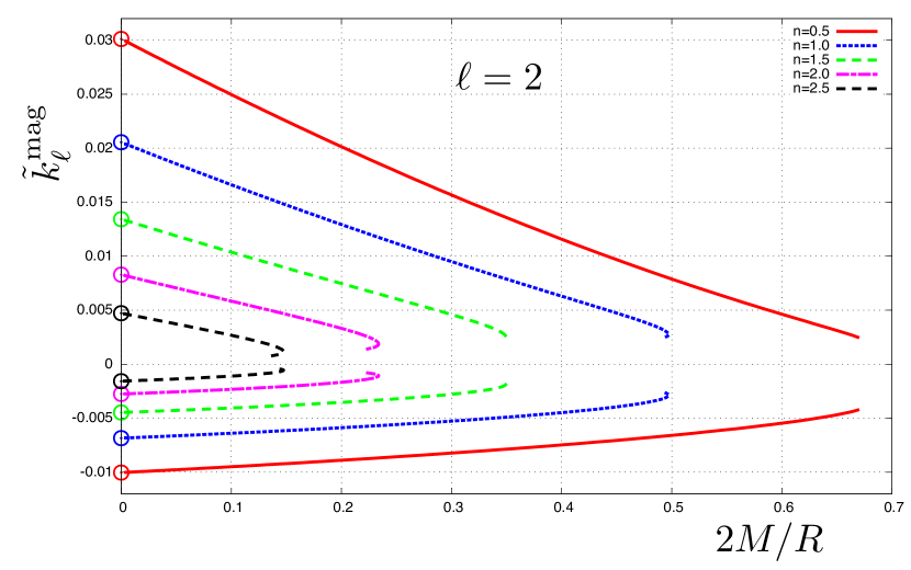
The gravitomagnetic Love numbers depend on the details of the body’s internal structure, as determined by its equation of state, which we take to be of the zero-temperature form , , where is the rest-mass density, the pressure, and the density of internal energy. For concreteness we adopt a simple polytropic model , , where and are constants. A sample of our computations is displayed in Fig. 1, which plots
| (3) |
as a function of for and selected values of the polytropic index . We observe that the tidal response of an irrotational fluid is dramatically different from the response of a fluid in strict hydrostatic equilibrium: the gravitomagnetic Love numbers of an irrotational body are negative, while they are positive for a body in strict hydrostatic equilibrium. Both sets of Love numbers, however, share the properties that they decrease (in absolute value) with increasing and with increasing ; because increasing decreases for a given , and therefore produces a body that is more centrally dense, both properties are associated with the fact that a more compact body develops smaller multipole moments.
In Sec. VI we exploit the methods of post-Newtonian theory to calculate in the limit , for any equation of state. We obtain the simple expression
| (4) |
which can be evaluated explicitly once the equation of state is specified. The parameter tracks the internal motions associated with the fluid’s irrotational state; setting places the body in the irrotational state and gives rise to a negative for any and any equation of state, while setting places the body in a strict hydrostatic equilibrium and gives rise to a positive gravitomagnetic Love number. The post-Newtonian values appear as circled data points in Fig. 1, and we see that they accurately reproduce the limit of the relativistic curves.
We conclude this introduction with a restatement of our main message. A nonrotating body in a tidal interaction with remote matter is expected to be in an irrotational state for which internal motions get established over time. These internal motions have a dramatic influence on the body’s gravitomagnetic Love numbers: while they are positive in the strict hydrostatic equilibria examined in previous works, they are negative in the irrotational state. This effect is captured by the post-Newtonian expression of Eq. (4), which is valid in the limit for any equation of state.
II Unperturbed configuration
The unperturbed body is taken to be static and spherically symmetric, and to consist of a perfect fluid with rest-mass density , pressure , density of internal energy , and density of total energy . The background spacetime has a metric given by
| (5) |
with , in which and depend on the radial coordinate , and . The metric is a solution to the Einstein field equations with energy-momentum tensor
| (6) |
in which is the fluid’s velocity field, with only nonvanishing component . The metric functions are determined by
| (7) |
in which a prime indicates differentiation with respect to . In the vacuum exterior the field equations produce the Schwarzschild solution and . The body’s surface is situated at , as determined by the condition .
The conservation equation gives rise to the relativistic Euler equation,
| (8) |
where is the covariant acceleration, and the first law of thermodynamics,
| (9) |
For the unperturbed configuration the only nonvanishing component of the acceleration vector is , and Eq. (8) reduces to
| (10) |
the Tolman-Oppenheimer-Volkov equation.
III Perturbed configuration
We next allow the fluid configuration to be perturbed by a time-dependent, external tidal field. The metric becomes , and the fluid quantities are shifted to , , , , and . We work consistently to first order in the perturbation, and note that .
Normalization of the perturbed velocity vector in the perturbed metric implies that , or . The remaining components are denoted and , with . We let and find that the components of are given by
| (11) |
A straightforward computation further reveals that
| (12a) | ||||
| (12b) | ||||
| (12c) | ||||
The perturbed configuration is governed by Euler’s equation, which becomes
| (13) |
after the perturbation. With the information provided above, we find that the radial component reads
| (14) |
while the angular components take the form of
| (15) |
The time component of Euler’s equation returns a trivial .
IV Irrotational configuration
The circulation of a relativistic fluid around a closed curve is defined by
| (16) |
where is the specific enthalpy defined by , and is the coordinate increment along . It is known that is the same for any circuit that surrounds a given fluid world tube. (The world tube can be thought of as a bundle of streamlines, defined as the world lines of fluid elements.) Thus, if surrounds the world tube at a time , and if surrounds the same world tube at a time , then and the circulation is conserved. A proof of the circulation theorem can be found in Synge’s 1937 review of relativistic hydrodynamics synge:37 .
Because for the unperturbed configuration, we have that the unperturbed fluid is irrotational: for any purely spatial circuit . The circulation of the perturbed configuration is then
| (17) |
We assume that the fluid begins in an unperturbed state, so that the perturbation vanishes at some initial time . This implies that for any circuit tangent to the hypersurface . Conservation of circulation then guarantees that the perturbed fluid is irrotational at all times: for any circuit tangent to any hypersurface . And because the integral of must vanish for any circuit , we conclude that an irrotational fluid configuration must satisfy
| (18) |
at all times. Importing Eq. (11), we have that
| (19) |
for an irrotational configuration.
We next insert the second of Eqs. (19) within Eq. (15). The equation integrates to
| (20) |
and this can be substituted back into Eq. (14), along with the first of Eqs. (19). This yields
| (21) |
With the help of Eq. (10) these expressions become
| (22) |
These equations imply that a spherical surface of constant or at radius in the unperturbed configuration is deformed by the perturbation to a nonspherical surface at . Equations (22) are a consequence of the perturbed Euler equation and the conservation of circulation for an irrotational fluid. They allow the perturbation to be time-dependent, but they are identical in form to the equations of hydrostatic equilibrium derived, for example, by Landry and Poisson landry-poisson:14 .
We are interested in the deformation of a fluid body placed in a tidal environment, and we shall henceforth assume that the tidal field varies slowly with time. In this context, the state of the fluid is at all times an approximate hydrostatic equilibrium described by Eqs. (22), in which all quantities vary slowly with time. The fluid, however, is not taken to be in a strict hydrostatic equilibrium, which would imply the complete absence of internal motions. Instead, the fluid is assumed to be in an irrotational state, which implies the existence of a velocity field described by Eq. (19). The internal motions are established even when the time dependence of the tidal field is arbitrarily slow. By contrast, the strict hydrostatic equilibrium previously studied by Damour and Nagar damour-nagar:09 and Binnington and Poisson binnington-poisson:09 can only be established when the tidal field is strictly time-independent. As such, it represents a much less realistic configuration for the perturbed fluid.
V Gravitomagnetic Love numbers of an irrotational compact body
In this section we determine the impact of the internal motions described by Eq. (19) on the body’s response to an applied tidal field, as measured by the gravitomagnetic Love numbers ; we shall show that they have no impact on the body’s gravitoelectric response. We assume that the tidal environment varies slowly with time, and neglect all time derivatives in the equations that determine the metric perturbation . But while the slow time dependence is assumed not to have an impact on the field equations, it is crucial in the establishment of the internal motions, as was explained in the preceding section.
To proceed we introduce a decomposition of into tensorial spherical harmonics. Denoting and , we have
| (23a) | ||||
| (23b) | ||||
| (23c) | ||||
in which , , , , , and depend on only, and
| (24a) | ||||
| (24b) | ||||
| (24c) | ||||
| (24d) | ||||
are the vectorial and tensorial harmonics constructed from the standard spherical harmonics ; is the metric on a unit two-sphere, is the covariant derivative operator compatible with this metric, is the Levi-Civita tensor on the unit two-sphere, with components , and upper-case Latin indices are raised with , the matrix inverse to . The terms involving , , and in Eq. (23) constitute the even-parity sector of the perturbation, and the terms involving and constitute the odd-parity sector.
The body’s response to the applied tidal field is measured by the Love numbers and introduced by Binnington and Poisson binnington-poisson:09 . Because these are gauge-invariant in the usual sense of perturbation theory, we may calculate them in any gauge, and for this purpose it is convenient to adopt the Regge-Wheeler gauge, for which , , and are all set equal to zero. The field equations further imply that , and we find that Eqs. (19) become
| (25) |
in Regge-Wheeler gauge. This implies that the internal motions associated with the irrotational state affect only the odd-parity sector of the perturbation. This, in turn, implies that the body’s gravitoelectric response to the tidal field is unaffected by the internal motions, but that there is an impact on the gravitomagnetic response. In other words, the internal motions do influence the gravitomagnetic Love numbers , but they leave the gravitoelectric Love numbers unchanged with respect to a strict hydrostatic equilibrium. We have inserted a factor in Eq. (25) to track the impact of the internal motions on the computation of ; setting would place the fluid in a strict hydrostatic equilibrium.
The computation of the gravitomagnetic Love numbers proceeds as detailed in Ref. binnington-poisson:09 and streamlined in Ref. landry-poisson:14 . The only change concerns the additional contribution to , the perturbation of the fluid’s energy-momentum tensor, created by the internal motions described by Eq. (25). Focusing on the odd-parity sector, writing
| (26) |
and making use of Eqs. (11) and (25), we find that the only relevant component is
| (27) |
With this, the Einstein field equations linearized about the unperturbed solution of Sec. II imply that the perturbation fields are determined by
| (28) |
where
| (29a) | ||||
| (29b) | ||||
We observe that the switch from strict hydrostatic equilibrium to an irrotational state changes the sign of the term in .
Equation (28) is to be integrated outward from , near which the solution behaves as . The internal solution is matched at to the external solution provided by Binnington and Poisson binnington-poisson:09 ,
| (30) |
where
| (31a) | ||||
| (31b) | ||||
with denoting the hypergeometric function, and is the spherical-harmonic packaging of the tidal moments introduced in Eq. (1), defined by
| (32) |
in which .
A practical formulation of this procedure was provided by Landry and Poisson landry-poisson:14 . It involves introducing the logarithmic derivative , which satisfies the nonlinear differential equation
| (33) |
This equation is integrated from , at which , to , at which . The matching condition at produces
| (34) |
with
| (35) |
in which a prime indicates differentiation with respect to . The overall scaling of with differs from the convention adopted in Damour and Nagar damour-nagar:09 and Binnington and Poisson binnington-poisson:09 , who introduced instead a scalefree Love number via the relation . The missing factor of was incorporated in Eq. (35), and it ensures that tends to a nonzero value in the limit ; this is unlike , which goes to zero in the limit.
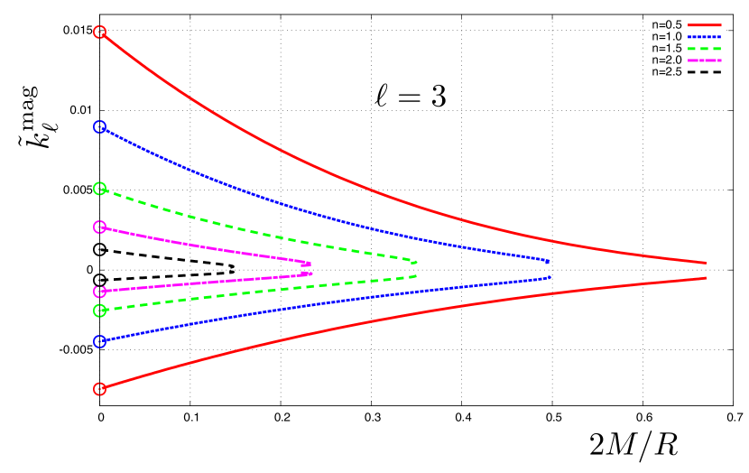
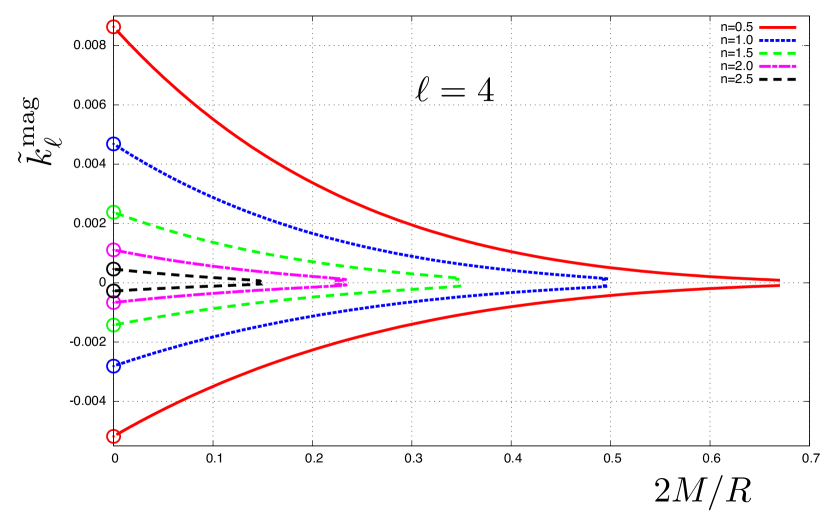
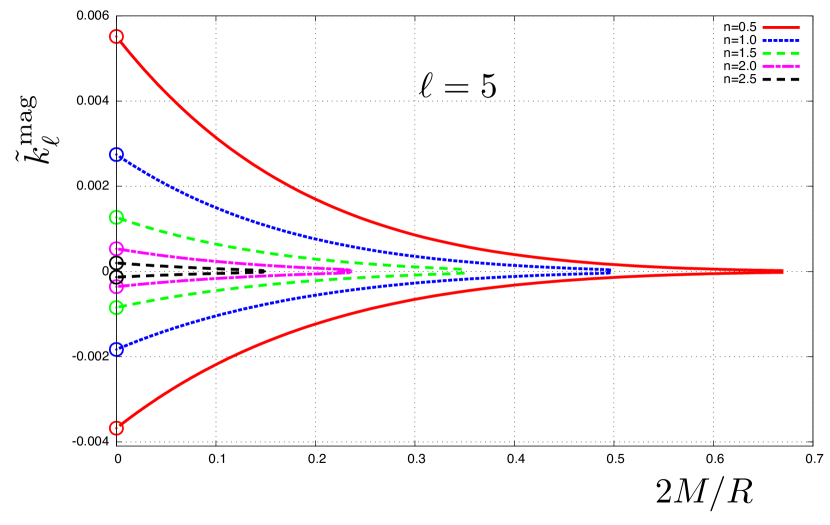
In Figs. 1–4 we present sample calculations of the rescaled gravitomagnetic Love numbers for a polytropic equation of state , , where and are constants. The details of integrating Eq. (33) for this specific case are presented in Appendix A. We see from the figures that the tidal response of an irrotational body is dramatically different from the response of a body in strict hydrostatic equilibrium: the gravitomagnetic Love numbers of an irrotational body are negative, while they are positive for a body in strict hydrostatic equilibrium. The change of sign can be seen to originate from the term in . Both sets of Love numbers, however, share the properties that they decrease (in absolute value) with increasing and with increasing polytropic index ; because increasing decreases for a given , and therefore produces a body that is more centrally dense, both properties are associated with the fact that a more compact body develops smaller multipole moments.
VI Post-Newtonian calculation of the gravitomagnetic Love numbers
In this section we exploit the methods of post-Newtonian theory to calculate the gravitomagnetic response of a weakly self-gravitating body to an applied tidal field. Our calculation returns an expression for that reproduces the leading-order behavior of the relativistic function when the body’s compactness is small. In this section we restore powers of and , which were set equal to unity in the preceding sections.
The post-Newtonian metric is expressed in harmonic coordinates as
| (36) |
and it involves a vector potential in addition to the familiar Newtonian potential , which satisfies the Poisson equation . The post-Newtonian terms of order in are not required in our developments, and the second post-Newtonian terms of order in are absorbed into .
As was described in Sec. I, the tidal environment is taken to be a pure gravitomagnetic -pole field characterized by the symmetric-tracefree (STF) tensor , which is assumed to vary slowly with time, so that we may neglect time derivatives in the field equations. The tidal field is described by the vector potential
| (37) |
where is the completely antisymmetric permutation symbol, , and . The STF nature of the tidal moment ensures that the vector potential satisfies Laplace’s equation as well as the harmonic gauge condition . It also implies that the vector potential can be expressed in the alternative form
| (38) |
in which and the angular brackets indicate the operation of trace-removal. It is easy to show that a transformation to spherical polar coordinates brings the metric to the form displayed in Eq. (30), in which we set to respect the post-Newtonian approximation, and because the body’s response has not yet been incorporated within the vector potential.
The body’s response to the applied tidal field is governed by the post-Newtonian Euler equation and the field equation satisfied by the vector potential. The relevant aspects can be collected from the textbook by Poisson and Will poisson-will:14 . From their Eq. (7.15b), in which we neglect the time derivatives, and their Eq. (7.23b) we obtain
| (39) |
in which the domain of integration is truncated to , where is a cutoff radius to be specified below. The body’s response is captured by the Poisson integral, and the integrand involves the effective current density which incorporates both a matter and field contribution. An expression for this is displayed in Exercise 8.4 of Poisson and Will; we have
| (40) |
in which we neglect a term involving in the field contribution to the mass current, as well as the terms multiplying because, as we shall see presently, the velocity field is itself of order . Our expression for should be multiplied by the factor arising from Eq. (7.23b) of Poisson and Will. This factor can be neglected when it multiplies the Poisson integral, but it produces a relativistic correction to . We shall not be interested in such corrections, and choose to drop the factor all together.
The velocity field is determined by the irrotational condition that we wish to place on the fluid. Writing for the four-velocity, in which is a normalization factor, a short computation reveals that the circulation of a post-Newtonian fluid around any spatial circuit is given by
| (41) |
An irrotational state therefore requires
| (42) |
This expression agrees with results previously obtained by Shapiro shapiro:96 and Favata favata:06 .
The calculation of the body’s response proceeds by inserting Eq. (42) within Eq. (40), and replacing by in this expression. We find that the velocity contribution to the mass current is given by
| (43) |
and that the field contribution is
| (44) |
To arrive at the last expression we recalled the fact that for a spherical body, , in which is the mass inside a sphere of radius . We also inserted a factor of in Eq. (43) to again track the influence of the internal motions on the body’s gravitomagnetic response.
The next step is to evaluate the Poisson integral in Eq. (39). The calculation requires the addition theorem for spherical harmonics,
| (45) |
in which and , and the identity displayed in Eq. (1.171) of Poisson and Will,
| (46) |
Evaluation of the Poisson integral for is straightforward, and when we obtain
| (47) |
in which
| (48) |
is a dimensionless moment of the mass density. In this case the domain of integration is naturally limited to the volume occupied by the body, and the cutoff radius is irrelevant. It does, however, play a role in the Poisson integral for , which features the radial integral
| (49) |
To evaluate this for we break up the integration domain into a first segment in which , , and is unspecified, a second segment in which , , and , and a third segment in which , , and . We obtain
| (50) |
To simplify this we integrate the first term by parts, making use of the Newtonian field equation . We also discard the term proportional to , because it merely gives rise to an uninteresting correction of order to the tidal potential of Eq. (37). The term proportional to can be seen to alter the amplitude of the tidal potential by a correction of order , and we eliminate this meaningless shift by setting . With all this we find that
| (51) |
and completing the evaluation of the Poisson integral, we arrive at
| (52) |
Adding the contributions, we find that the body’s gravitomagnetic response to the applied tidal field is described by
| (53) |
The complete vector potential is , and comparison with Eq. (1) reveals the post-Newtonian expression for the gravitomagnetic Love numbers. Recalling Eq. (48), we find that
| (54) |
with
| (55) |
We recall that keeps track of the internal motions associated with the fluid’s irrotational state. Setting places the body in the irrotational state, and we observe that negative gravitomagnetic Love numbers must be assigned to such a body, irrespective of the multipole order and the equation of state. By contrast, setting places the body in a strict hydrostatic equilibrium, and such a body necessarily comes with positive gravitomagnetic Love numbers. These properties were featured in the fully relativistic results displayed in Figs. 1–4, and indeed, we observe that the post-Newtonian expression of Eq. (55) accurately reproduces the relativistic Love numbers in the limit .
Our post-Newtonian calculation of the gravitomagnetic Love numbers completes previous attempts carried out by Favata favata:06 and Damour and Nagar damour-nagar:09 . In his work (see Sec. III B of his paper), Favata introduces a definition for the Love numbers that accounts only for the velocity term in the effective mass current; it omits the field term , and Favata therefore produces only the term in Eq. (55). On the other hand, the post-Newtonian calculation of Damour and Nagar (see Sec. VIII of their paper) places the fluid in a strict hydrostatic equilibrium instead of the irrotational state, and therefore accounts only for the -independent term in Eq. (55). (It should be noted that the Damour-Nagar definition for the gravitomagnetic Love numbers includes a multiplicative minus sign compared to ours; their Love numbers are negative when ours are positive.) Our own calculation brings the two partial stories together, and generalizes the previous calculations (which were limited to ) to arbitrary multipole order .
Equation (55) can be evaluated in closed form in a few simple cases. For a constant density body we find that
| (56) |
For an Newtonian polytrope, for which , we have that
| (57a) | ||||
| (57b) | ||||
| (57c) | ||||
| (57d) | ||||
The numerical values correspond to and , respectively.
Acknowledgements.
One of us (EP) is grateful to the Canadian Institute of Theoretical Astrophysics for its warm hospitality during a research leave from the University of Guelph. This work was supported by the Natural Sciences and Engineering Research Council of Canada.Appendix A Structure and perturbation equations for polytropes
To perform the computations described in Sec. V for the polytropic equation of state , we recast the background field equations of Sec. II and Eq. (33) in convenient, dimensionless forms. To achieve this we introduce the central density , the central pressure , the length scale defined by , and the mass scale . A useful dimensionless parameter is , which can act as a substitute for the central density as a label of polytropic models. A frequently encountered combination of scaling quantities is .
We next introduce the dimensionless, Lane-Emden-type variables , , and , such that , , , , and . The equations that determine the internal structure of the unperturbed polytrope are then
| (58) |
and
| (59) |
with . An equation can also be displayed for the gravitational potential , but this is not needed to calculate the Love numbers. The integrations begin at with and . They proceed until at which and . The body’s compactness can then be calculated as . In the limit the equations reduce to the standard Lane-Emden form.
The dimensionless version of Eq. (33) is
| (60) |
with
| (61a) | ||||
| (61b) | ||||
The integration begins at with and proceeds until at which .
In practice it is helpful to use as the independent variable, and to start the integration at a large, negative value of . Starting values for , and can be obtained from the Taylor expansions , , and , in which the various coefficients can be determined from the differential equations.
References
- (1) E. E. Flanagan and T. Hinderer, Constraining neutron star tidal Love numbers with gravitational wave detectors, Phys. Rev. D 77, 021502(R) (2008), arXiv:0709.1915.
- (2) T. Hinderer, Tidal Love numbers of neutron stars, Astrophys. J. 677, 1216 (2008), erratum: Astrophys. J. 697, 964 (2009), arXiv:0711.2420.
- (3) T. Hinderer, B. D. Lackey, R. N. Lang, and J. S. Read, Tidal deformability of neutron stars with realistic equations of state and their gravitational wave signatures in binary inspiral, Phys. Rev. D 81, 123016 (2010), arXiv:0911.3535.
- (4) L. Baiotti, T. Damour, B. Giacomazzo, A. Nagar, and L. Rezzolla, Analytic modeling of tidal effects in the relativistic inspiral of binary neutron stars, Phys. Rev. Lett. 105, 261101 (2010), arXiv:1009.0521.
- (5) L. Baiotti, T. Damour, B. Giacomazzo, A. Nagar, and L. Rezzolla, Accurate numerical simulations of inspiralling binary neutron stars and their comparison with effective-one-body analytical models, Phys. Rev. D 84, 024017 (2011), arXiv:1103.3874.
- (6) J. Vines, E. E. Flanagan, and T. Hinderer, Post-1-Newtonian tidal effects in the gravitational waveform from binary inspirals, Phys. Rev. D 83, 084051 (2011), arXiv:1101.1673.
- (7) F. Pannarale, L. Rezzolla, F. Ohme, and J. S. Read, Will black hole-neutron star binary inspirals tell us about the neutron star equation of state?, Phys. Rev. D 84, 104017 (2011), arXiv:1103.3526.
- (8) B. D. Lackey, K. Kyutoku, M. Shibata, P. R. Brady, and J. L. Friedman, Extracting equation of state parameters from black hole-neutron star mergers. I. Nonspinning black holes, Phys. Rev. D 85, 044061 (2012), arXiv:1109.3402.
- (9) T. Damour, A. Nagar, and L. Villain, Measurability of the tidal polarizability of neutron stars in late-inspiral gravitational-wave signals, Phys. Rev. D 85, 123007 (2012), arXiv:1203.4352.
- (10) J. S. Read, L. Baiotti, J. D. E. Creighton, J. L. Friedman, B. Giacomazzo, K. Kyutoku, C. Markakis, L. Rezzolla, M. Shibata, and K. Taniguchi, Matter effects on binary neutron star waveforms, Phys. Rev. D 88, 044042 (2013), arXiv:1306.4065.
- (11) J. E. Vines and E. E. Flanagan, First-post-Newtonian quadrupole tidal interactions in binary systems, Phys. Rev. D 88, 024046 (2013), arXiv:1009.4919.
- (12) B. D. Lackey, K. Kyutoku, M. Shibata, P. R. Brady, and J. L. Friedman, Extracting equation of state parameters from black hole-neutron star mergers: Aligned-spin black holes and a preliminary waveform model, Phys. Rev. D 89, 043009 (2014), arXiv:1303.6298.
- (13) M. Favata, Systematic parameter errors in inspiraling neutron star binaries, Phys. Rev. Lett. 112, 101101 (2014), arXiv:1310.8288.
- (14) K. Yagi and N. Yunes, Love number can be hard to measure, Phys. Rev. D 89, 021303 (2014), arXiv:1310.8358.
- (15) S. A. Hughes, Evolution of circular, nonequatorial orbits of Kerr black holes due to gravitational-wave emission. II. Inspiral trajectories and gravitational waveforms, Phys. Rev. D 64, 064004 (2001), arXiv:gr-qc/0104041.
- (16) R. H. Price and J. T. Whelan, Tidal interaction in binary-black-hole inspiral, Phys. Rev. Lett. 87, 231101 (2001), arXiv:gr-qc/0107029.
- (17) K. Martel, Gravitational waveforms from a point particle orbiting a Schwarzschild black hole, Phys. Rev. D 69, 044025 (2004), arXiv:gr-qc/0311017.
- (18) N. Yunes, A. Buonanno, S. A. Hughes, M. C. Miller, and Y. Pan, Modeling extreme mass ratio inspirals within the effective-one-body approach, Phys. Rev. Lett. 104, 091102 (2010), arXiv:0909.4263.
- (19) N. Yunes, A. Buonanno, S. A. Hughes, Y. Pan, E. Barausse, M. C. Miller, and W. Throwe, Extreme mass-ratio inspirals in the effective-one-body approach: Quasicircular, equatorial orbits around a spinning black hole, Phys. Rev. D 83, 044044 (2011), arXiv:1009.6013.
- (20) K. Chatziioannou, E. Poisson, and N. Yunes, Tidal heating and torquing of a Kerr black hole to next-to-leading order in the tidal coupling, Phys. Rev. D 87, 044022 (2013), arXiv:1211.1686.
- (21) D. Bini, T. Damour, and G. Faye, Effective action approach to higher-order relativistic tidal interactions in binary systems and their effective one body description, Phys. Rev. D 85, 124034 (2012), arXiv:1202.3565.
- (22) S. Chakrabarti, T. Delsate, and J. Steinhoff, New perspectives on neutron star and black hole spectroscopy and dynamic tides (2013), arXiv:1304.2228.
- (23) S. Chakrabarti, T. Delsate, and J. Steinhoff, Effective action and linear response of compact objects in Newtonian gravity, Phys. Rev. D 88, 084038 (2013), arXiv:1306.5820.
- (24) S. R. Dolan, P. Nolan, A. C. Ottewill, N. Warburton, and B. Wardell, Tidal invariants for compact binaries on quasicircular orbits, Phys. Rev. D 91, 023009 (2015), arXiv:1406.4890.
- (25) D. Bini and T. Damour, Gravitational self-force corrections to two-body tidal interactions and the effective one-body formalism, Phys. Rev. D 90, 124037 (2014), arXiv:1409.6933.
- (26) E. Poisson and C. M. Will, Gravity: Newtonian, Post-Newtonian, Relativistic (Cambridge University Press, Cambridge, England, 2014).
- (27) M. Favata, Are neutron stars crushed? Gravitomagnetic tidal fields as a mechanism for binary-induced collapse, Phys. Rev. D 73, 104005 (2006), arXiv:astro-ph/0510668.
- (28) T. Damour and A. Nagar, Relativistic tidal properties of neutron stars, Phys. Rev. D 80, 084035 (2009), arXiv:0906.0096.
- (29) T. Binnington and E. Poisson, Relativistic theory of tidal Love numbers, Phys. Rev. D 80, 084018 (2009), arXiv:0906.1366.
- (30) S. L. Shapiro, Gravitomagnetic Induction during the Coalescence of Compact Binaries, Phys. Rev. Lett. 77, 4487 (1996).
- (31) X.-H. Zhang, Multipole expansions of the general-relativistic gravitational field of the external universe, Phys. Rev. D 34, 991 (1986).
- (32) J. L. Synge, Relativistic hydrodynamics, Proc. London Math. Soc. 43, 376 (1937).
- (33) P. Landry and E. Poisson, Relativistic theory of surficial Love numbers, Phys. Rev. D 89, 124011 (2014), arXiv:1404.6798.