WxBS: Wide Baseline Stereo Generalizations

Abstract

We present a generalization of the wide baseline two view matching problem - WxBS, where x stands for a different subset of “wide baselines" in acquisition conditions such as geometry, illumination, sensor and appearance. We introduce a novel dataset of ground-truthed image pairs which include multiple "wide baselines" and show that state-of-the-art matchers fail on almost all image pairs from the set. A novel matching algorithm for addressing the WxBS problem is introduced and we show experimentally that the WxBS-M matcher dominates the state-of-the-art methods both on the new and existing datasets.

1 Introduction

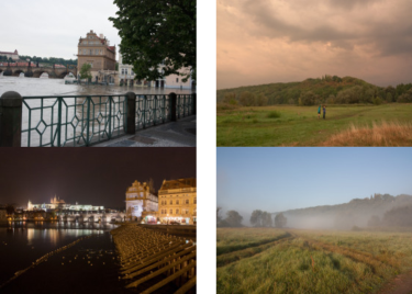
Figure 1: Examples of WxBS problems.

The Wide Baseline Stereo (WBS) matching problem, first formulated by Pritchett and Zisserman [Pritchett and Zisserman(1998)], has received significant attention in the last 15 years [Mikolajczyk et al.(2005)Mikolajczyk, Tuytelaars, Schmid, Zisserman, Matas, Schaffalitzky, Kadir, and Van Gool, Tuytelaars and Mikolajczyk(2008)]. Progressively more challenging two- and multi-view problems have been successfully handled [Tuytelaars and Mikolajczyk(2008)] and recent algorithms [Morel and Yu(2009)], [Mishkin et al.(2015)Mishkin, Perdoch, and Matas] have shown impressive performance, e.g. matching views of planar objects with orientation difference of up to 160 degrees.

Besides the orientation and viewpoint baseline, other factors influence the complexity of establishing geometric correspondence between a pair of images. The standard physical models of image formation and acquisition consider, beside geometry, the effects of illumination, the properties of the transparent medium light rays pass through in the scene, the surface properties of objects and the properties of the imaging sensors.

In the paper, we consider the generalization of Wide (geometric) Baseline Stereo to WxBS, a two-view image matching problem where two or more of the image formation and acquisition properties significantly change, i.e. they have a wide baseline. The "significant change" distinguishes the problem from image registration, where dense correspondence is routinely established between multi-modal images and various complex transformations have been considered, see Zitová and Flusser [Zitova and Flusser(2003)]. Operationally, the "wide baseline" means "where local, gradient-descent type" methods fail.

The following single wide baseline stereo, or correspondence, problems and their combinations are considered: illumination (WlBS) – difference in position, direction, number, intensity and wavelength of light sources; geometry (WgBS) – difference in camera and object pose, scale and resolution - the “classical” WBS; sensor (WsBS) – change in sensor type: visible, IR, MR; noise, image preprocessing algorithms inside the camera, etc; appearance (WaBS) – difference in the object appearance because of time or seasonal changes, occlusions, turbulent air, etc. We denote matching problems, or, equivalently, image pairs, with a significant change in only one of the groups listed as W1BS; if a combination of effects is present, as WxBS. To our knowledge, almost all published image datasets and algorithms are in the W1BS class[Mikolajczyk et al.(2005)Mikolajczyk, Tuytelaars, Schmid, Zisserman, Matas, Schaffalitzky, Kadir, and Van Gool], [Morel and Yu(2009)], [Vonikakis et al.(2013)Vonikakis, Chrysostomou, Kouskouridas, and Gasteratos],[Aguilera et al.(2012)Aguilera, Barrera, Lumbreras, Sappa, and Toledo],[Hauagge and Snavely(2012)], [Jacobs et al.(2007)Jacobs, Roman, and Pless].

We present a new public dataset with ground truth which combines the above-mentioned challenges and contains both W2BS image pairs including viewpoint and appearance, viewpoint and illumination, viewpoint and sensor, illumination and appearance change and W3BS – problems where viewpoint, appearance and lighting differ significantly.

We show that state-of-the-art matchers performs poorly on the introduced image matching pairs, and propose a novel algorithm which significantly outperforms the state-of-the-art without a dramatic loss of speed.

The paper is organised as follows. In Section 2, relevant datasets and matching algorithms are reviewed. The novel WxBS matching algorithm is then introduced in Section 4. The dataset for WxBS problems and the associated evaluation protocol are presented in Section 3. Experimental results are described in Section 5. The paper is concluded in Section 6.

2 Related Work

Viewpoint change. The stereo problem – matching of two images taken from different viewpoints – has always received significant attention of the computer vision community as it is a critical component of the structure from motion task. For images taken concurrently, in both the calibrated and uncalibrated set up, the problem for a narrow baseline is mature [Tuytelaars and Mikolajczyk(2008)] and can be now solved in real-time and on a large scale [Agarwal et al.(2009)Agarwal, Snavely, Simon, Seitz, and Szeliski].

For wide-baseline matching, the standard evaluation protocol focuses on the feature detection and description stages[Mikolajczyk et al.(2005)Mikolajczyk, Tuytelaars, Schmid, Zisserman, Matas, Schaffalitzky, Kadir, and Van Gool]. However, the methodology and datasets of [Mikolajczyk et al.(2005)Mikolajczyk, Tuytelaars, Schmid, Zisserman, Matas, Schaffalitzky, Kadir, and Van Gool] are limited to images related by a homography. Attempts have been made to extend the evaluation to 3D scenes [Moreels and Perona(2005), Aanæs et al.(2012)Aanæs, Dahl, and Pedersen], but they are significantly less popular. Neither of the above-mentioned protocols evaluates the performance of the matching stage and thus of the full matching pipeline.

As a reference, we adopted two recent algorithms which reported good performance and whose binaries are freely available. The ASIFT method [Morel and Yu(2009)] method synthetically transforms images in order to improve the range of affine transformations of the DoG detector. This idea have been further extended in MODS [Mishkin et al.(2013)Mishkin, Perdoch, and Matas] which incorporates multiple detectors and adopts an iterative approach that attempts to minimize the matching time. Both algorithms are able to match images with extreme viewpoint changes. Mishkin et al [Mishkin et al.(2013)Mishkin, Perdoch, and Matas] introduced an extreme-viewpoint dataset that is used to test the ability of the newly proposed WxBS matcher to handle viewpoint changes.

Multimodal image analysis is needed for the alignment of images acquired by different sensors. Most commonly, the problem is encountered in remote sensing and in medical imaging. For instance, in [Ghassabi et al.(2013)Ghassabi, Shanbehzadeh, Sedaghat, and Fatemizadeh], red-free and fluorescein angiographic images are matched. Similarly for different modes of magnetic resonance imaging, modality of the captured data depends on the magnetic properties of the scanned chemical compound. In remote sensing, multimodal matching involves, e.gregistering visual spectrum images against near infrared images (NIR) or Long-Wave infrared (LWIR).

Multimodal registration methods are usually divided to area-based and feature-based methods. As we are interested in extending the challenges into multiple-baseline variations, area-based methods are omitted as they lack scale invariance [Ghassabi et al.(2013)Ghassabi, Shanbehzadeh, Sedaghat, and Fatemizadeh].

Feature-based approaches [Vonikakis et al.(2013)Vonikakis, Chrysostomou, Kouskouridas, and Gasteratos] and [Ghassabi et al.(2013)Ghassabi, Shanbehzadeh, Sedaghat, and Fatemizadeh] identify the main issues of existing algorithms in the context of multimodal matching as the selection of the the response threshold, i.e. the minimal image contrast which triggers the detector. In [Vonikakis et al.(2013)Vonikakis, Chrysostomou, Kouskouridas, and Gasteratos], the Difference of Gaussian (DoG) [Lowe(2004)] response is normalised by local average image intensity in cases when the image contrast is low. Ghassabi et al [Ghassabi et al.(2013)Ghassabi, Shanbehzadeh, Sedaghat, and Fatemizadeh] present a variant of the DoG detector which sets a local response threshold for each image cell on the basis of the image entropy. In [Chen et al.(2010)Chen, Tian, Lee, Zheng, Smith, and Laine], it is argued that Harris detector is more suitable for this task as the information along boundaries is preserved in cases of different image modalities.

The main issue of the widely used SIFT descriptor [Lowe(2004)] in the context of multimodal images is the lack of invariance to gradient reversal. Two approaches to address this issue have been proposed in the literature. The first generates a second SIFT descriptor of the feature for a gradient reversed image by SIFT vector reordering [Hare et al.(2011)Hare, Samangooei, and Lewis]. We refer to this method as inverted-SIFT. The second method [Chen et al.(2010)Chen, Tian, Lee, Zheng, Smith, and Laine], denoted as half-SIFT, limits local image gradients directions to $\langle 0,\pi)$ by merging opposite gradient directions in orientation estimation. Unlike the inverted-SIFT, this method allows matching of images that are only partially inverted (per patch),i.e.some gradient directions stay the same while other are reversed. The downside is the reduction of the descriptor discriminability.

The computation of inverted-SIFT has a negligible computational cost, as it can be generated from SIFT descriptors by rearranging the data in the gradient histogram. The only associated computational cost is in the matching since twice as many features are matched in the second image. For the half-SIFT method, the feature patch and its descriptor has to be extracted as the dominant feature orientation differs from SIFT’s dominant orientation.

An example of a multimodal image registration dataset is presented in [Aguilera et al.(2012)Aguilera, Barrera, Lumbreras, Sappa, and Toledo]. This dataset consist of 100 pairs of vertically aligned images from a camera and a LWIR thermal sensor. The viewpoint changes between related image pairs are negligible.

Change in object illumination and appearance. Techniques similar to those developed for multimodal image matching can be used for matching of images of differently illuminated objects. In [Kelman et al.(2007)Kelman, Sofka, and Stewart], the authors employ half-SIFT and further modify SIFT descriptor in such a way that it collects only gradients located on edges. Yang et al [Yang et al.(2007)Yang, Stewart, Sofka, and Tsai] use the Difference of Gaussian features and SIFT to estimate the transformation between the images. If no matches are found, an identity transformation is assumed. From a single local match, multiscale features together with local image statistics are used in an iterative procedure called Dual-Bootstrap to enlarge the region of good alignment. A data presented in [Kelman et al.(2007)Kelman, Sofka, and Stewart] are used in Section 5.

Hauagge et al [Hauagge and Snavely(2012)] argue that local symmetries survive significant illumination changes and developed a higher-level feature detector for matching of urban scenes where symmetries are abundant. They also assume that the vertical direction is aligned with one of the edges of the image. The method proposed in [Hauagge and Snavely(2012)] is able to match images of architectural objects taken many years apart and even sketches to photos. The dataset introduced in the paper contains 46 pairs of images.

Matching of images depicting very different appearance of the same object arise in computer vision applications. A system for guided drawing of free-form objects called Shadow-Draw is presented in [Lee et al.(2011)Lee, Zitnick, and Cohen]. It can be seen as a large-scale image retrieval system which interactively tries to look for images based on sketches given by a user. In the object classification field, the multiple-appearance problem has been investigated in [Shrivastava et al.(2011)Shrivastava, Malisiewicz, Gupta, and Efros] who train a data-driven visual similarity measure in order to match images to sketches or paintings. Those two approaches use global image description rather than local image feature matching.

3 Datasets

Datasets used in experiments are listed in Table 1. When evaluating detectors (Section 5) and the proposed matching algorithm (Section 4) all dataset images are used. However, descriptor evaluation is performed only on a subset of the most challenging and prominent pairs (i.e. only pairs 1-6 from OxfordAffine) with provided homography of each WxBScategory.

Most of the published datasets (with exception of the LostInPast dataset [Fernando et al.(2014)Fernando, Tommasi, and Tuytelaars]) include only a single nuisance factor per image pair. This is suitable for evaluation of the robustness to a particular nuisance factor but fails to predict performance in more complex environments. One of the motivations of the proposed WxBS datasets is to address this issue.

Table 1: Datasets used for evaluation

Short name	Proposed by	#images	Type
GDB	Kelman et al [Kelman et al.(2007)Kelman, Sofka, and Stewart], 2007	22 pairs	WlBS, WsBS
SymB	Hauagge and Snavely [Hauagge and Snavely(2012)], 2012	46 pairs	WaBS, WlBS
MMS	Aguilera et al [Aguilera et al.(2012)Aguilera, Barrera, Lumbreras, Sappa, and Toledo], 2012	100 pairs	WsBS
EVD	Mishkin et al [Mishkin et al.(2013)Mishkin, Perdoch, and Matas], 2013	15 pairs	WgBS
OxAff	Mikolajczyk et al[Mikolajczyk et al.(2005)Mikolajczyk, Tuytelaars, Schmid, Zisserman, Matas, Schaffalitzky, Kadir, and Van Gool], [Mikolajczyk and Schmid(2005)], 2013	8 sixplets	WgBS
EF	Zitnick and Ramnath et al[Zitnick and Ramnath(2011)],2011	8 sixplets	WgBS,WlBS
Amos	Jacobs et al[Jacobs et al.(2007)Jacobs, Roman, and Pless],2007	$>$ 100K	WlBS,WaBS
VPRiCE	VPRICE Challenge 2015 [Suenderhauf and Glover(2015)]	3K pairs	WgaBS, WglBS,WgsBS,
Past	Fernando et al[Fernando et al.(2014)Fernando, Tommasi, and Tuytelaars], 2014	502 images	WgaBS
WxBS	here	37 pairs	WaBS,WgaBS,WglBS, WgsBS,WlaBS,WgalBS

WxBS dataset and evaluation protocol. A set of 37 image pairs has been collected from Flickr and other sources. The dataset is divided into 6 categories based on the combinations of nuisance factor present, see Table 2. For every image, a set of approximately 20 ground-truth correspondences has been annotated. Selected examples are presented in Figure 2. The resolution of the majority of the images is $800\times 600$ with the exception of LWIR images from the WgsBS dataset which were captured by a thermal camera with a resolution of $250\times 250$ pixels. The selected image pairs contain both urban and natural scenes.

Table 2: The WxBS datasets categories

Short name	Nuisance	#images	Avg. # GT Corr.
map2ph	appearance (map to photo)	6 pairs	homography provided
WgaBS	viewpoint, appearance	5 pairs	22 per img.
WglBS	viewpoint, lighting	9 pairs	21 per img.
WgsBS	viewpoint, modality	5 pairs	18 per img.
WlaBS	lighting, appearance	4 pairs	25 per img.
WgalBS	viewpoint, appearance, lighting	8 pairs	17 per img.

Figure 2: Examples of image pairs from the WxBS dataset.

Ground truth and the evaluation protocol. In the image registration tasks, it is often sufficient to define ground truth as a homography between an image pair. However, the WxBS dataset contains significant viewpoint changes. In the case of a non-planar scene a homography can, at best, cover the dominant plane.

We assume that an ideal algorithm matches the majority of the scene content, thus our ground truth is a set of manually selected correspondences which evenly cover the part of the scene visible in both images. The average number of correspondences per image pair is shown in Table 2.

The evaluation protocol for the WxBS dataset.

For each image pair indexed with $i\in\mathbb{Z}$ we have manually annotated a set of correspondences $(\mathbf{u}_{i},\mathbf{v}_{i})\in C_{i}$ where $\mathbf{u}$ and $\mathbf{v}$ are positions in the 1^st and the 2^nd image respectively. For epipolar geometry we use the symmetric epipolar distance and the symmetric reprojection error for homography [Hartley and Zisserman(2000)].

Recall on ground truth correspondences $C_{i}$ of image pair $i$ and for geometry model $\mathbf{M}_{i}$ is computed as a function of a threshold $\theta$

$$\mathrm{r}_{i,\mathbf{M}_{i}}(\theta)=\frac{|(\mathbf{u}_{i},\mathbf{v}_{i}):(\mathbf{u}_{i},\mathbf{v}_{i})\in C_{i},e(\mathbf{M}_{i},\mathbf{u},\mathbf{v})<\theta|}{|C_{i}|}$$ (1)

using appropriate error functions. For all pairs of each category $W$ we define an overall recall per category as:

$$\mathrm{r}_{W}(\theta)=\frac{1}{|W|\sum_{i\in W}\mathrm{r}_{i,M_{i}}(\theta)}$$ (2)

This measure is as the fraction of the confirmed annotated correspondences for a given threshold in a nuisance category.

Algorithm 1 MODS-WxBS – a matcher for wide multiple baseline stereo

$I_{1}$, $I_{2}$ – two images; $\theta_{m}$ – minimum required number of matches; $S_{\text{max}}$ – maximum number of iterations.

Fundamental or homography matrix F or H;

a list of corresponding local features.  

while $(N_{\text{matches}}<\theta_{m})$ ${\mathit{a}nd}$ $(\text{Iter}<S_{\text{max}})$ do

    for $I_{1}$ and $I_{2}$ separately do

        1 Generate synthetic views according to the

        scale-tilt-rotation-detector setup for the Iter.

        2 Detect local features using adaptive threshold.

        3 Extract rotation invariant descriptors with:

        3a rSIFT    and    3b hrSIFT

        4 Reproject local features to $I_{1}$.

    end for

    5 Generate tent. corresp. based on the first geom.

        inconsistent rule for rSIFT and hrSIFT

        separately using kD-tree

    6 Filter duplicates

    7 Geometric verification of all TC with modified

        DEGENSAC estimating $F$ or $H$.

    8 Check geom. consistency of the LAFs

with est. $F$.

end while

4 Matching algorithm for wide multiple baseline stereo

In this section, we propose a variant of MODS [Mishkin et al.(2013)Mishkin, Perdoch, and Matas, Mishkin et al.(2015)Mishkin, Perdoch, and Matas] matcher designed for WxBS problems called WxBS-MODS, or WxBS-M in short. Its overall structure is shown in Algorithm 1. The view synthesis is identical to the original MODS framework [Mishkin et al.(2013)Mishkin, Perdoch, and Matas].

Tentative correspondences are generated using kD-tree [Muja and Lowe(2014)] and the 1st geometrically inconsistent rule with radius equal 10 pixels as threshold is applied[Mishkin et al.(2013)Mishkin, Perdoch, and Matas]. Descriptors from different detectors types (Hessian, MSER+, MSER-) as well as for different descriptors are put in seperate kD-trees. After matching, all tentative correspondences are put into a single list and duplicates, which appears due to view synthesis, are filtered if features in both images are within a 3 pixel radius.

5 Evaluation of description and detection algorithms

In this section, multiple detection and description algorithms are evaluated.

Descriptors evaluation. The evaluation protocol is as follows. The dataset consists of 40 image pairs from datasets listed in Table 1 divided into 5 parts by the nuisance factor. For all pairs, homography is the appropriate two-view relationship – the images are either without significant relative depth of taken from virtually identical viewpoints. In order to minimize bias towards a specific detector, affine-covariant regions by Hessian-Affine, MSER and FOCI in the first – least challenging image of the pair are used (visible in case of IR-vis, day on day-night, frontal when view point changes, etc.). The affine-covariant regions have been detected with dominant orientation and then reprojected to the second image by the ground truth homography. Features which are not visible in the second image have been discarded. Therefore geometric repeatability of affine regions on the selected regions is always $100\%$ and the maximum possible recall is 1. Color-to-grayscale image transformation have been done via channel averaging, which gives best matching performance [Kanan and Cottrell(2012)].

Then affine regions were normalized to patch size 41x41 (scale $\sigma=3\sqrt{3}$) and described with given descriptors. An affine-normalization procedure is performed even for the fast binary descriptors, which is rarely used because of the significant additional processing time. However, the goal of our experiment is to explore descriptor performance in challenging conditions, not their speed. The procedure helps – the typical threshold of the Hamming distance for binary descriptors on unnormalized patch is around 60-80, while on affine normalized patches similar performance is obtained with a threshold around 10-30. All descriptors clearly benefit from the affine-normalized process, e.g. the graffiti 1-6 pair from the OxfordAffine dataset could be matched with FREAK descriptor only when using a normalized patch.

The tested descriptors are: SIFT [Lowe(2004)], rSIFT [Arandjelović and Zisserman(2012)], hrSIFT (gradients in interval $\left[0;\pi\right)$) [Kelman et al.(2007)Kelman, Sofka, and Stewart], InvSIFT (SIFT with reordered cells as for inverted image) [Hare et al.(2011)Hare, Samangooei, and Lewis], LIOP[Zhenhua Wang and Wu(2011)], AKAZE [Alcantarilla et al.(2013)Alcantarilla, Nuevo, and Bartoli], MROGH [Fan et al.(2012)Fan, Wu, and Hu], FREAK [Alahi et al.(2012)Alahi, Ortiz, and Vandergheynst], ORB [Rublee et al.(2011)Rublee, Rabaud, Konolige, and Bradski], SymFeat [Hauagge and Snavely(2012)], SSIM [Shechtman and Irani(2007)] (implementation [Chatfield et al.(2009)Chatfield, Philbin, and Zisserman]), DAISY [Tola et al.(2010)Tola, Lepetit, and Fua] and $L_{2}$-normalized raw grayscale pixel intensities.

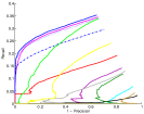
(a) WGBS

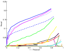
(b) WLBS

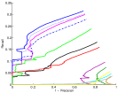
(c) WLBS

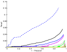
(d) WSBS

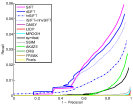
(e) map2ph

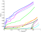
(f) all

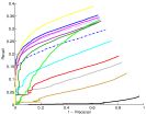
(g) WGBS

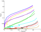
(h) WLBS

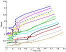
(i) WLBS

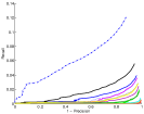
(j) WSBS

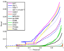
(k) map2ph

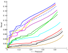
(l) all

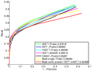
(m) WGBS

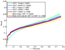
(n) WLBS

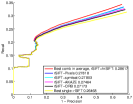
(o) WLBS

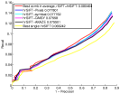
(p) WSBS

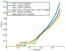
(q) map2ph

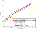
(r) all

Figure 3: First row: descriptors computed using authors’ implementation, second row - descriptors computed on photometrically normalized patches (mean = 0.5, var = 0.2) patches as done in SIFT. Third row: top 5 complementary pairs of descriptors (photometrically normalized). The numbers in legend are mean average precision. Bottom row: examples of the image pairs from each subset. Note that axis scales differs in each column, i.e. for different WxBS problems.

Floating point descriptors have been compared using $L_{2}$ distance, binary using Hamming distance. The Recall-Precision curves are shown in Figure 3. The second-nearest distance ratio is used to parameter the curve for floating point descriptors, the Hamming distance for binary ones.

Note that most of the descriptors gain significantly from photometric normalization, cf. the first two rows of Figure 3. The published implementations are clearly sensitivite to contrast variations.

The results hows that gradient-histogram based SIFT and its variants including DAISY are the best performing descriptors by a big margin in the presence of any (geometric, illumination, etc) nuisance factors despite the fact that some of the competitors – LIOP, MROGH – have been specifically designed to deal with illumination changes. The second best descriptor is – surprisingly – the patch with contrast-$L_{2}$-normalized pixels, which beats all other descriptors. It has huge memory footprint – 1681 floats, but the affine-photo-$L_{2}$-normed grayscale pixel intensities are a strong descriptor baseline.

Most of descriptors, despite their different underlying assumptions and algorithmic structure, successfully match almost the same patches (see third row in Figure 3) – and the most complementary descriptor to the leading rSIFT is its gradient-reversal-insensitive version – hrSIFT.

The results confirming the domination of SIFT-based methods are in agreement with [Stylianou et al.(2015)Stylianou, Abrams, and Pless] and [Fernando et al.(2014)Fernando, Tommasi, and Tuytelaars] despite the fact that they adopted a rather different evaluation methodology. However, we could not confirm clear superiority of the SSIM over SymFeat descriptors, which could be explained by the fact that the SSIM descriptor was designed for use only with the SSIM detector. Detectors evaluation. The following detectors are compared: MSER [Matas et al.(2002)Matas, Chum, Urban, and Pajdla], DoG [Lowe(2004)], Hessian-Affine [Mikolajczyk and Schmid(2004)] (implementation [Perdoch et al.(2009)Perdoch, Chum, and Matas]), FOCI [Zitnick and Ramnath(2011)], IIDOG [Vonikakis et al.(2013)Vonikakis, Chrysostomou, Kouskouridas, and Gasteratos], WADE [Salti et al.(2013)Salti, Lanza, and Di Stefano], W$\alpha$SH [Varytimidis et al.(2012)Varytimidis, Rapantzikos, and Avrithis], SURF [Bay et al.(2006)Bay, Tuytelaars, and Gool], SFOP [Förstner et al.(2009)Förstner, Dickscheid, and Schindler], AKAZE[Alcantarilla et al.(2013)Alcantarilla, Nuevo, and Bartoli]. We focus on getting a reliable answer to the "match/non-match" question in real image pairs. Therefore the performance criterion is the number of successfully matched pairs using the best combination of descriptors (see Section Descriptors evaluation ) –  rSIFT and hrSIFT. Matching is done as in Algorithm 1 except that no view synthesis is performed. Image pairs are considered matched if $\geq$15 correct inliers to a homography are found. Since the Lost-in-past dataset contains 2300 matchable image pairs, which is unfeasible for direct matching, we have selected a subset of 172 medium-challenging image pairs. Other datasets are used fully.

Adaptive threshold of the detector response. One of the main problems in matching of day to night and infrared images is the low number of detected features. The problem is acute in dark low contrast images in the WgsBS and MMS [Aguilera et al.(2012)Aguilera, Barrera, Lumbreras, Sappa, and Toledo] datasets. A possible approach addressing the problem is iiDoG [Vonikakis et al.(2013)Vonikakis, Chrysostomou, Kouskouridas, and Gasteratos] where the difference of Gaussians is normalized by sum of Gaussians. It works well, but cannot be easily applied for other types of detectors, i.e. MSER.

Table 3: Detector evaluation results. The number of matched image pairs (left) and the average running time (right). The FOCI detector is run through MS Windows simulator wine, the time includes a big overhead.

Alg.	EF		EVD		MMS		WgaBS		WgalBS		WglBS		WgsBS		WlaBS		Past		OxAff		SymB		GDB
	# 33	time $[s]$	# 15	time $[s]$	# 100	time $[s]$	# 5	time $[s]$	# 8	time $[s]$	# 9	time $[s]$	# 5	time $[s]$	# 4	time $[s]$	# 172	time $[s]$	# 40	time $[s]$	# 46	time $[s]$	# 22	time $[s]$
Threshold adaptation
MSER	black!16!black!1616	1.4	black!303	1.4	black!11	0.3	black!000	2.0	black!000	1.3	black!000	1.3	black!000	0.8	black!101	1.2	black!88	1.3	black!40!black!4040	3.5	black!23!black!2323	2.4	black!99	2.4
AdMSER	black!25!black!2525	3.4	black!808	4.0	black!66	1.0	black!000	4.0	black!000	3.2	black!000	3.3	black!000	1.4	black!101	2.6	black!1111	2.9	black!40!black!4040	5.7	black!26!black!2626	4.6	black!1313	6.9
DoG	black!29!black!2929	2.3	black!000	2.8	black!1010	0.8	black!000	2.7	black!000	2.3	black!000	2.1	black!000	1.0	black!101	2.4	black!1313	2.0	black!38!black!3838	4.8	black!29!black!2929	2.7	black!1212	4.7
iiDoG	black!29!black!2929	3.1	black!000	3.0	black!1111	1.2	black!000	3.2	black!000	2.9	black!000	2.8	black!000	1.2	black!101	2.5	black!1313	2.2	black!38!black!3838	8.0	black!29!black!2929	2.9	black!1212	6.1
AdDoG	black!29!black!2929	2.6	black!000	3.4	black!1111	1.2	black!000	3.3	black!000	3.0	black!000	3.0	black!000	1.5	black!101	2.7	black!1313	2.7	black!38!black!3838	4.1	black!30!black!3030	3.0	black!1212	4.8
HesAf	black!32!black!3232	4.6	black!101	5.2	black!1515	1.2	black!000	5.5	black!000	3.8	black!000	4.2	black!000	2.0	black!101	3.6	black!2424	4.0	black!40!black!4040	11.	black!35!black!3535	5.8	black!1717	9.1
AdHesAf	black!33!black!3333	5.7	black!202	7.6	black!3535	2.9	black!000	7.2	black!101	6.5	black!000	6.0	black!000	3.2	black!101	4.9	black!2525	5.4	black!40!black!4040	10.	black!35!black!3535	7.2	black!1818	13.
Other detectors
W$\alpha$SH	black!0!black!00	1.8	black!000	5.4	black!00	0.6	black!000	2.8	black!000	2.5	black!000	1.4	black!000	1.8	black!000	1.2	black!00	1.9	black!24!black!2424	4.1	black!3!black!33	2.8	black!33	6.9
ORB	black!3!black!33	4.1	black!000	3.6	black!11	0.8	black!000	2.8	black!000	2.7	black!000	3.6	black!000	1.6	black!000	2.8	black!11	2.3	black!28!black!2828	8.7	black!5!black!55	3.0	black!33	6.1
SURF	black!27!black!2727	2.3	black!000	2.4	black!77	1.0	black!000	2.5	black!000	1.9	black!000	2.1	black!000	0.9	black!101	1.4	black!1010	1.9	black!38!black!3838	5.8	black!31!black!3131	2.9	black!1515	4.0
AKAZE	black!28!black!2828	4.3	black!000	3.6	black!1010	0.8	black!101	4.7	black!000	3.4	black!000	4.0	black!000	1.3	black!101	2.7	black!2525	3.6	black!38!black!3838	13.	black!35!black!3535	5.6	black!1717	6.4
FOCI	black!29!black!2929	12.	black!000	39.	black!1414	11.	black!101	32.	black!000	29.	black!000	29.	black!000	20.	black!101	29.	black!2121	13.	black!38!black!3838	35.	black!35!black!3535	27.	black!1717	45.
SFOP	black!25!black!2525	11.	black!000	16.	black!1212	4.7	black!000	12.	black!000	10.	black!000	10.	black!000	9.2	black!000	7.5	black!1111	12.	black!36!black!3636	15.	black!24!black!2424	11.	black!88	17.
WADE	black!16!black!1616	14.	black!000	20.	black!00	3.4	black!000	58.	black!000	11.	black!000	14.	black!000	7.9	black!101	8.3	black!2020	23.	black!34!black!3434	60.	black!34!black!3434	46.	black!1313	77.
State-of-art matchers
ASIFT	black!23!black!2323	27.	black!505	12.	black!1818	3.2	0	52.	0	32.	0	35.	0	12.	black!101	30.	black!6262	32.	black!40!black!4040	102	black!27!black!2727	14.	black!1515	41.
MODS	black!33!black!3333	4.8	black15	11.	black!2727	11.	black!202	41.	black!202	31.	black!101	46.	black!000	17.	black!101	26.	black!9494	27.	black!40!black!4040	3.4	black!42!black!4242	18.	black!1818	11.
DBstrap	black!31!black!3131	26.	0	18.	black!7979	9.3	0	11.	0	13.	0	13.	0	4.7	0	15.	black!1616	28.	black!36!black!3636	24.	black!38!black!3838	21.	black!1616	17.
Proposed matcher
WXBS-M	black!33!black!3333	4.7	black15	14.	black!8282	12.	black!303	40.	black!303	63.	black!303	61.	black!000	26.	black!303	28.	black107	42.	black!40!black!4040	5.1	black!43!black!4343	18.	black22	12.

Instead, we propose to use the following adaptive thresholding for all feature detectors. First, all local extrema of the response function are detected (i.e. no thresholding takes place). Next, the detected features are sorted according to the response magnitude. If the number of detected features with response magnitude $\geq$ $\Theta$ is greater than a given threshold $R_{\text{min}}$, these are output and the algorithm terminates (this is the standard approach). If there is not enough features above the threshold, top $R_{\text{min}}$ features our output.

Discussion and results. The performance of the proposed WxBS-M matcher is compared with it state-of-art matchers: ASIFT [Morel and Yu(2009)], Dual Bootstrap (DBstrap) [Yang et al.(2007)Yang, Stewart, Sofka, and Tsai] and MODS [Mishkin et al.(2015)Mishkin, Perdoch, and Matas] on various WxBS problems.

The results are summarized in Table 5. Note that the state-of-the-art matchers were not able to match almost any image pair which combines more nuisance factors. The proposed WxBS-M matcher shows much better performance, but still is not able to solve even half of the new dataset pairs.

Results in Table 5 confirm that the proposed adaptive thresholding strategy works as well as, or even better, than iiDoG for DoG, but it is 1.5 times faster. It also significantly improves results of the MSER and Hessian-Affine, even when main the nuisance is in the viewing geometry (EVD dataset).

6 Conclusions

We have presented a new problem – the wide multiple baseline stereo (WxBS) – which considers matching of images that simultaneously differ in more than one image acquisition factor such as viewpoint, illumination, sensor type or where object appearance changes significantly, e.g. over time. A new dataset with the ground truth for evaluation of matching algorithms has been introduced and will be made public.

We have extensively tested a large set of popular and recent detectors and descriptors and show than the combination of RootSIFT and HalfRootSIFT as descriptors with MSER and Hessian-Affine detectors works best for many different nuisance factors. We show that simple adaptive thresholding improves Hessian-Affine, DoG, MSER (and possibly other) detectors and allows to use them on infrared and low contrast images.

A novel matching algorithm for addressing the WxBS problem has been introduced. We have shown experimentally that the WxBS-M matcher dominantes the state-of-the-art methods both on both the new and existing datasets.

References

- [Aanæs et al.(2012)Aanæs, Dahl, and Pedersen] Henrik Aanæs, Anders Lindbjerg Dahl, and Kim Steenstrup Pedersen. Interesting interest points. IJCV 2012, pages 18–35, 2012.
- [Agarwal et al.(2009)Agarwal, Snavely, Simon, Seitz, and Szeliski] S. Agarwal, N. Snavely, I. Simon, S.M. Seitz, and R. Szeliski. Building rome in a day. In ICCV 2009, pages 72–79, 2009.
- [Aguilera et al.(2012)Aguilera, Barrera, Lumbreras, Sappa, and Toledo] Cristhian Aguilera, Fernando Barrera, Felipe Lumbreras, Angel D Sappa, and Ricardo Toledo. Multispectral image feature points. Sensors, 12(9):12661–12672, 2012.
- [Alahi et al.(2012)Alahi, Ortiz, and Vandergheynst] Alexandre Alahi, Raphael Ortiz, and Pierre Vandergheynst. FREAK: Fast Retina Keypoint. In CVPR 2012, 2012.
- [Alcantarilla et al.(2013)Alcantarilla, Nuevo, and Bartoli] P. F. Alcantarilla, J. Nuevo, and A. Bartoli. Fast explicit diffusion for accelerated features in nonlinear scale spaces. In BMVC 2013, 2013.
- [Arandjelović and Zisserman(2012)] R. Arandjelović and A. Zisserman. Three things everyone should know to improve object retrieval. In CVPR 2012, 2012.
- [Bay et al.(2006)Bay, Tuytelaars, and Gool] Herbert Bay, Tinne Tuytelaars, and Luc Van Gool. Surf: Speeded up robust features. In ECCV 2006, pages 404–417, 2006.
- [Chatfield et al.(2009)Chatfield, Philbin, and Zisserman] K. Chatfield, J. Philbin, and A. Zisserman. Efficient retrieval of deformable shape classes using local self-similarities. In Workshop on Non-rigid Shape Analysis and Deformable Image Alignment, ICCV, 2009.
- [Chen et al.(2010)Chen, Tian, Lee, Zheng, Smith, and Laine] Jian Chen, Jie Tian, N. Lee, Jian Zheng, R.T. Smith, and A.F. Laine. A partial intensity invariant feature descriptor for multimodal retinal image registration. IEEE Transactions on Biomedical Engineering, 57(7):1707–1718, 2010.
- [Fan et al.(2012)Fan, Wu, and Hu] Bin Fan, Fuchao Wu, and Zhanyi Hu. Rotationally invariant descriptors using intensity order pooling. PAMI 2012, 34(10):2031–2045, 2012.
- [Fernando et al.(2014)Fernando, Tommasi, and Tuytelaars] Basura Fernando, Tatiana Tommasi, and Tinne Tuytelaars. Lost in the past: Recognizing locations over large time lags. CoRR, abs/1409.7556, 2014.
- [Förstner et al.(2009)Förstner, Dickscheid, and Schindler] W. Förstner, T. Dickscheid, and F. Schindler. Detecting interpretable and accurate scale-invariant keypoints. In 12th IEEE International Conference on Computer Vision (ICCV’09), Kyoto, Japan, 2009.
- [Ghassabi et al.(2013)Ghassabi, Shanbehzadeh, Sedaghat, and Fatemizadeh] Zeinab Ghassabi, Jamshid Shanbehzadeh, Amin Sedaghat, and Emad Fatemizadeh. An efficient approach for robust multimodal retinal image registration based on ur-sift features and piifd descriptors. EURASIP Journal on Image and Video Processing, (1):1–16, 2013.
- [Hare et al.(2011)Hare, Samangooei, and Lewis] Jonathon S. Hare, Sina Samangooei, and Paul H. Lewis. Efficient clustering and quantisation of sift features: Exploiting characteristics of the sift descriptor and interest region detectors under image inversion. In ICMR 2011, pages 2:1–2:8. ACM, 2011.
- [Hartley and Zisserman(2000)] Richard Hartley and Andrew Zisserman. Multiple view geometry in computer vision. Cambridge University Press, 2000.
- [Hauagge and Snavely(2012)] D.C. Hauagge and N. Snavely. Image matching using local symmetry features. In CVPR 2012, pages 206–213, 2012.
- [Jacobs et al.(2007)Jacobs, Roman, and Pless] Nathan Jacobs, Nathaniel Roman, and Robert Pless. Consistent Temporal Variations in Many Outdoor Scenes. In CVPR 2007, 2007.
- [Kanan and Cottrell(2012)] Christopher Kanan and Garrison W. Cottrell. Color-to-grayscale: Does the method matter in image recognition? PLoS ONE, 2012.
- [Kelman et al.(2007)Kelman, Sofka, and Stewart] Avi Kelman, Michal Sofka, and Charles V Stewart. Keypoint descriptors for matching across multiple image modalities and non-linear intensity variations. In CVPR 2007, 2007.
- [Lee et al.(2011)Lee, Zitnick, and Cohen] Yong Jae Lee, C Lawrence Zitnick, and Michael F Cohen. Shadowdraw: real-time user guidance for freehand drawing. In ACM Transactions on Graphics (TOG), volume 30, page 27. ACM, 2011.
- [Lowe(2004)] David G. Lowe. Distinctive image features from scale-invariant keypoints. IJCV 2004, 60(2):91–110, 2004.
- [Matas et al.(2002)Matas, Chum, Urban, and Pajdla] J. Matas, O. Chum, M. Urban, and T. Pajdla. Robust wide baseline stereo from maximally stable extrema regions. In BMVC 2002, pages 384–393, 2002.
- [Mikolajczyk and Schmid(2005)] K. Mikolajczyk and C. Schmid. A performance evaluation of local descriptors. PAMI 2005, 27(10):1615–1630, 2005.
- [Mikolajczyk and Schmid(2004)] Krystian Mikolajczyk and Cordelia Schmid. Scale & affine invariant interest point detectors. IJCV 2004, 60(1):63–86, 2004.
- [Mikolajczyk et al.(2005)Mikolajczyk, Tuytelaars, Schmid, Zisserman, Matas, Schaffalitzky, Kadir, and Van Gool] Krystian Mikolajczyk, Tinne Tuytelaars, Cordelia Schmid, Andrew Zisserman, Jiri Matas, Frederik Schaffalitzky, Timor Kadir, and Luc Van Gool. A comparison of affine region detectors. IJCV 2005, 65(1-2):43–72, 2005.
- [Mishkin et al.(2013)Mishkin, Perdoch, and Matas] Dmytro Mishkin, Michal Perdoch, and Jiri Matas. Two-view matching with view synthesis revisited. In IVCNZ 2013, pages 436–441, 2013.
- [Mishkin et al.(2015)Mishkin, Perdoch, and Matas] Dmytro Mishkin, Michal Perdoch, and Jiri Matas. Mods: Fast and robust method for two-view matching. CoRR, abs/1503.02619, 2015.
- [Moreels and Perona(2005)] P. Moreels and P. Perona. Evaluation of features detectors and descriptors based on 3d objects. In CVPR 2005, volume 1, pages 800–807 Vol. 1, 2005.
- [Morel and Yu(2009)] Jean-Michel Morel and Guoshen Yu. Asift: A new framework for fully affine invariant image comparison. SIAM Journal on Imaging Sciences, 2(2):438–469, 2009.
- [Muja and Lowe(2014)] M. Muja and D. Lowe. Scalable nearest neighbour algorithms for high dimensional data. PAMI 2014, PP(99):1–1, 2014.
- [Perdoch et al.(2009)Perdoch, Chum, and Matas] M. Perdoch, O. Chum, and J. Matas. Efficient representation of local geometry for large scale object retrieval. In CVPR 2009, pages 9–16, 2009.
- [Pritchett and Zisserman(1998)] P. Pritchett and A. Zisserman. Wide baseline stereo matching. In ICCV 1998, pages 754–760, 1998.
- [Rublee et al.(2011)Rublee, Rabaud, Konolige, and Bradski] E. Rublee, V. Rabaud, K. Konolige, and G. Bradski. Orb: An efficient alternative to sift or surf. In ICCV 2011, pages 2564–2571, 2011.
- [Salti et al.(2013)Salti, Lanza, and Di Stefano] Samuele Salti, Alessandro Lanza, and Luigi Di Stefano. Keypoints from symmetries by wave propagation. In CVPR 2013, pages 2898–2905, 2013.
- [Shechtman and Irani(2007)] Eli Shechtman and Michal Irani. Matching local self-similarities across images and videos. In CVPR 2007, 2007.
- [Shrivastava et al.(2011)Shrivastava, Malisiewicz, Gupta, and Efros] Abhinav Shrivastava, Tomasz Malisiewicz, Abhinav Gupta, and Alexei A Efros. Data-driven visual similarity for cross-domain image matching. In ACM Transactions on Graphics (TOG), volume 30, page 154. ACM, 2011.
- [Stylianou et al.(2015)Stylianou, Abrams, and Pless] A. Stylianou, A. Abrams, and R. Pless. Characterizing feature matching performance over long time periods. In WACV 2015, pages 892–898, 2015.
- [Suenderhauf and Glover(2015)] Niko Suenderhauf and Arren Glover. The vprice challenge 2015: Visual place recognition in changing environments, 2015. URL https://roboticvision.atlassian.net/wiki/pages/viewpage.action?pageId=14188617.
- [Tola et al.(2010)Tola, Lepetit, and Fua] E. Tola, V. Lepetit, and P. Fua. DAISY: An Efficient Dense Descriptor Applied to Wide-Baseline Stereo. PAMI 2010, 32(5):815–830, 2010.
- [Tuytelaars and Mikolajczyk(2008)] Tinne Tuytelaars and Krystian Mikolajczyk. Local Invariant Feature Detectors: A Survey. Now Publishers Inc., 2008.
- [Varytimidis et al.(2012)Varytimidis, Rapantzikos, and Avrithis] C. Varytimidis, K. Rapantzikos, and Y. Avrithis. Wash: Weighted -shapes for local feature detection. In ECCV 2012, 2012.
- [Vonikakis et al.(2013)Vonikakis, Chrysostomou, Kouskouridas, and Gasteratos] Vasillios Vonikakis, Dimitrios Chrysostomou, Rigas Kouskouridas, and Antonios Gasteratos. A biologically inspired scale-space for illumination invariant feature detection. Measurement Science and Technology, 24(7), 2013.
- [Yang et al.(2007)Yang, Stewart, Sofka, and Tsai] Gehua Yang, Charles V Stewart, Michal Sofka, and Chia-Ling Tsai. Registration of challenging image pairs: Initialization, estimation, and decision. PAMI 2007, 29(11):1973–1989, 2007.
- [Zhenhua Wang and Wu(2011)] Bin Fan Zhenhua Wang and Fuchao Wu. Local intensity order pattern for feature description. In ICCV 2011, pages 603–610, 2011.
- [Zitnick and Ramnath(2011)] C. Lawrence Zitnick and Krishnan Ramnath. Edge foci interest points. In ICCV 2011, pages 359–366, 2011.
- [Zitova and Flusser(2003)] Barbara Zitova and Jan Flusser. Image registration methods: a survey. Image and Vision Computing, 21(11):977 – 1000, 2003.