Digital Backpropagation in the
Nonlinear Fourier Domain

Abstract

Nonlinear and dispersive transmission impairments in coherent fiber-optic communication systems are often compensated by reverting the nonlinear Schrödinger equation, which describes the evolution of the signal in the link, numerically. This technique is known as digital backpropagation. Typical digital backpropagation algorithms are based on split-step Fourier methods in which the signal has to be discretized in time and space. The need to discretize in both time and space however makes the real-time implementation of digital backpropagation a challenging problem. In this paper, a new fast algorithm for digital backpropagation based on nonlinear Fourier transforms is presented. Aiming at a proof of concept, the main emphasis will be put on fibers with normal dispersion in order to avoid the issue of solitonic components in the signal. However, it is demonstrated that the algorithm also works for anomalous dispersion if the signal power is low enough. Since the spatial evolution of a signal governed by the nonlinear Schrödinger equation can be reverted analytically in the nonlinear Fourier domain through simple phase-shifts, there is no need to discretize the spatial domain. The proposed algorithm requires only $\mathcal{O}(D\log^{2}D)$ floating point operations to backpropagate a signal given by $D$ samples, independently of the fiber’s length, and is therefore highly promising for real-time implementations. The merits of this new approach are illustrated through numerical simulations.

I Introduction

The evolution of a signal $E(x,t)\in\mathbb{C}$ in optical fiber, where $x\geq 0$ denotes the position in the fiber and $t\in\mathbb{R}$ the time, is well-described through the nonlinear Schrödinger equation (NSE). Through proper scaling and coordinate transforms, the NSE can be brought into its normalized form

$$\operatorname{i}\frac{\partial E}{\partial x}+\frac{\partial^{2}E}{\partial t^{2}}+2\kappa|E|^{2}E=-\operatorname{i}\Gamma E,\quad\kappa\in\{\pm 1\}.$$ (1)

The parameter $\kappa$ in Eq. (1) effectively determines whether the fiber dispersion is normal ($-1$) or anomalous ($+1$), while the parameter $\Gamma$ determines the loss in the fiber. In the following, it will be assumed that the loss parameter is zero. There are two important cases in which a fiber-optic communication channel can be modeled under this assumption. When the fiber loss is mitigated through periodic amplification of the signal, the average of the properly transformed signal is known to satisfy the NSE with zero loss [1]. Furthermore, recently a distributed amplification scheme with an effectively unattenuated optical signal (quasi-lossless transmission directly described by the lossless NSE) has been demonstrated [2]. If the loss parameter is zero, the NSE can be solved using nonlinear Fourier transforms (NFTs) [3]. The spatial evolution of the signal $E(x,t)$ then reduces to a simple phase-shift in the nonlinear Fourier domain (NFD), similar to how linear convolutions reduce to phase-shifts in the conventional Fourier domain. The prospect of an optical communication scheme that inherently copes with the nonlinearity of the fiber has recently led to several investigations on how data can be transmitted in the NFD instead of the conventional Fourier or time domains [4, 5, 6, 7, 8, 9, 10, 11], with the original idea being due to Hasegawa and Nyu [12]. Next to potential savings in computational complexity, it is anticipated that subchannels defined in the NFD will not suffer from intra-channel interference, which is currently limiting the data rates achievable by wavelength-division multiplexing systems [13].

The mathematics behind the NFT are however quite involved, and despite recent progress in the implementation of fast forward and inverse NFTs [14, 15, 16] no integrated concept for a computationally efficient fiber-optic transmission system that operates in the NFD seems to be available. In this paper, therefore the problem of digital backpropagation (DBP), i.e. recovering the fiber input $E(0,t)$ from the output $E(x_{1},t)$ by solving (1), is addressed instead using NFTs [5]. Both concepts are compared in Fig. 1. Although DBP does not solve the issue of intra-channel interference in fiber-optic networks because it is usually not feasible to join the individual subchannels of the physically separated users into a single super-channel in this case [13, X.D], we note that there are other scenarios where this issue does not arise [17]. The advantage of digital backpropagation over information transmission in the NFD is that it is not necessary to implement full forward and backward NFTs. Together with recent advantages made in [14, 15, 16], this observation will enable us to perform digital backpropagation in the NFD using only $\mathcal{O}(D\log^{2}D)$ floating point operations (flops), where $D$ is the number of samples. This complexity estimate is independent of the length of the fiber because the spatial evolution of the signal will be carried out analytically. Conventional split-step Fourier methods, in contrast, have a complexity of $\mathcal{O}(MD\log D)$ flops, where $M$ is the number of spatial steps [18, III.G].

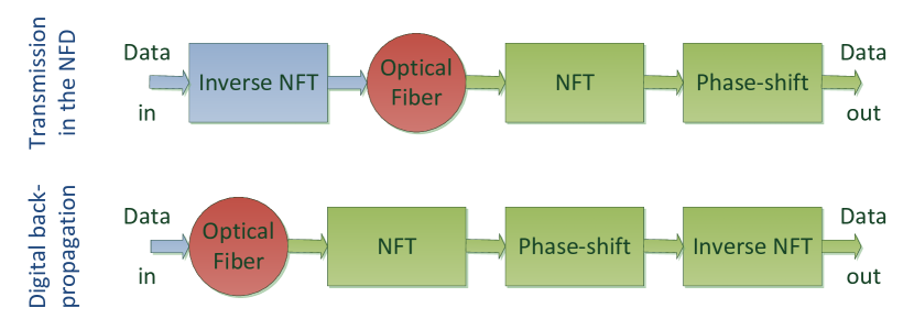
Figure 1: Information transmission (top) vs DBP (bottom) in the NFD

The goal of this paper is to present a new, fast algorithm for digital backpropagation that operates in the NFD and to compare it with traditional split-step Fourier methods through numerical simulations. The impact of noise resulting from the use of distributed Raman amplification will be of particular interest. The paper is structured as follows. In Sec. II, the theory behind digital backpropagation in the NFD will be outlined, and the new, fast algorithm will be given and discussed. The simulation setup is described in Sec. III, while results are reported in Sec. IV. Sec. V concludes the paper.

II Digital Backpropagation in the
Nonlinear Fourier Domain

In this section, first the theoretical and computational results that are required to perform digital backpropagation in the NFD are briefly recapitulated from [16]. Afterwards, the fast algorithm is presented and its limitations are discussed.

II-A Theory for the Continuous-Time Case

The Zakharov-Shabat scattering problem associated to any signal $E(x,t)$ that vanishes sufficiently fast for $t\to\pm\infty$ is

$$\frac{d}{dt}\boldsymbol{\mathbf{\phi}}(x,t,\lambda)= \left[\begin{array}[]{cc}-\operatorname{i}\lambda&E(x,t)\\ -\kappa\bar{E}(x,t)&\operatorname{i}\lambda\end{array}\right]\boldsymbol{\mathbf{\phi}}(x,t,\lambda),$$ (4)

$$\boldsymbol{\phi}(x,t,\lambda)= \left[\begin{array}[]{c}\operatorname{e}^{-\operatorname{i}\lambda t}\\ 0\end{array}\right]+o(1),\quad t\to-\infty.$$ (7)

With $\phi_{1}$ and $\phi_{2}$ denoting the components of $\boldsymbol{\phi}$, now define

$$\alpha(x,\lambda):= \lim_{t\to\infty}\operatorname{e}^{\operatorname{i}\lambda t}\phi_{1}(x,t,\lambda),$$ (8)

$$\beta(x,\lambda):= \lim_{t\to\infty}\operatorname{e}^{-\operatorname{i}\lambda t}\phi_{2}(x,t,\lambda),$$

where $\lambda\in\mathbb{C}$ is a parameter. If $E(x,t)$ satisfies the NSE (1) with zero loss parameter $\Gamma=0$, the corresponding $\alpha(x,\lambda)$ and $\beta(x,\lambda)$ turn out to depend on $x$ in very simple way:

$$\alpha(x,\lambda)=\alpha(0,\lambda),\quad\beta(x,\lambda)=\operatorname{e}^{-4\operatorname{i}\lambda^{2}x}\beta(0,\lambda).$$ (9)

These functions are not the final form of the NFT, but for our needs it will be sufficient to stop here.

The complicated spatial evolution of the signal $E(x,t)$ thus indeed becomes trivial if it is transformed into $\alpha(x,\lambda)$ and $\beta(x,\lambda)$. Based on this insight, ideal continuous-time digital backpropagation reduces to three basic steps in the NFD:

$$E(x_{1},t)\stackrel{{\scriptstyle\text{A}}}{{\to}}\left[\begin{array}[]{c}\alpha(x_{1},\lambda)\\ \beta(x_{1},\lambda)\end{array}\right]\stackrel{{\scriptstyle\text{B}}}{{\to}}\left[\begin{array}[]{c}\alpha(0,\lambda)\\ \beta(0,\lambda)\end{array}\right]\stackrel{{\scriptstyle\text{C}}}{{\to}}E(0,t).$$ (10)

II-B Discretization of the Continuous-Time Problem

In order to obtain a numerical approximation of $\alpha(x,\lambda)$ and $\beta(x,\lambda)$ for any fixed $x$, choose a sufficiently large interval $[T_{1},T_{2}]$ inside which $E(x,t)$ has already vanished sufficiently. Without loss of generality, one can assume that $T_{1}=-1$ and $T_{2}=0$. In this interval, $D$ rescaled samples

$$E[x,n]:=\epsilon E\left(x,-1+n\epsilon-\frac{\epsilon}{2}\right),\,\epsilon:=\frac{1}{D},\,n\in\{1,\dots,D\},$$

are taken. With $z:=\operatorname{e}^{-2\operatorname{i}\lambda\epsilon}$, (4)–(7) becomes

$$\boldsymbol{\phi}[x,n,z]:= z^{\frac{1}{2}}\left[\begin{array}[]{cc}1&z^{-1}E[x,n]\\ -\kappa\bar{E}[x,n]&z^{-1}\end{array}\right]$$ (13)

$$\times\frac{\boldsymbol{\phi}[x,n-1,z]}{\sqrt{1+\kappa|E[x,n]|^{2}}},$$ (14)

$$\boldsymbol{\phi}[x,0,z]:= z^{-\frac{D}{2}}\left[\begin{array}[]{c}1\\ 0\end{array}\right].$$ (17)

This leads to the following polynomial approximations:

$$\alpha(x,\lambda)\approx a(x,z):= {\textstyle\sum_{i=0}^{D-1}}a_{i}(x)z^{-i}:=\phi_{1}[x,D,z],$$

$$\beta(x,\lambda)\approx b(x,z):= {\textstyle\sum_{i=0}^{D-1}}b_{i}(x)z^{-i}:=\phi_{2}[x,D,z].$$

II-C The Algorithm

The three steps in the diagram (10) can be implemented with an overall complexity of $\mathcal{O}(D\log^{2}D)$ flops as follows.

Step A

The discrete scattering problem to find the polynomials $a(x_{1},z)$ and $b(x_{1},z)$ from the known fiber output $E(x_{1},t)$ through (14)–(17) is solved with only $\mathcal{O}(D\log^{2}D)$ flops using [15, Alg. 1] (also see [14, Alg. 1]).

Step B

The unknown polynomials $a(0,z)$ and $b(0,z)$ are defined by the unknown fiber input $E(0,t)$ through (14)–(17). In this step, approximations $\hat{a}(0,z)$ and $\hat{b}(0,z)$ of $a(0,z)$ and $b(0,z)$ are computed based on Eq. (9). The left-hand in (9) suggests the choice $\hat{a}(0,z):=\hat{a}(x_{1},z)$. For finding $\hat{b}(0,t)$, let us denote the $D$-th root of unity by $w:=\operatorname{e}^{-2\pi\operatorname{i}/D}$. The right-hand in (9) motivates us to find $\hat{b}(0,z)=\sum_{i=0}^{D-1}\hat{b}_{i}(0)z^{-i}$ by solving the well-posed interpolation problem

$$\hat{b}(0,w^{n-\frac{1}{2}})= \operatorname{e}^{4\operatorname{i}\left(\log(w^{n-\frac{1}{2}})/(-2\operatorname{i}\epsilon)\right)^{2}x_{1}}b(x_{1},w^{n-\frac{1}{2}})$$ (18)

$$= \operatorname{e}^{4\pi^{2}\operatorname{i}(n-\frac{1}{2})^{2}x_{1}}b(x_{1},w^{n-\frac{1}{2}}),\,n\in\{1,\dots,D\},$$

with the fast Fourier transform, using only $\mathcal{O}(D\log D)$ flops.

Step C

The inverse scattering problem of estimating $E[0,n]$ from $\hat{a}(0,z)$ and $\hat{b}(0,z)$ by inverting (14)–(17) is solved using $\mathcal{O}(D\log^{2}D)$ flops as described in [16, IV].

II-D Limitations

It was already mentioned above that the algorithm works for fibers with normal dispersion. In that case, the sign $\kappa$ in the NSE (1) will be negative and $E(x,t)$ is determined through the values that $\alpha(0,\lambda)$ and $\beta(0,\lambda)$ take on the real axis $\mathbb{R}\ni\lambda$ [19, p. 285]. If the dispersion is anomalous, the sign will be positive and $E(x,t)$ is determined through the values that $\alpha(0,\lambda)$ and $\beta(0,\lambda)$ take on the real axis and around the roots of $\alpha(0,\lambda)$ in the complex upper half-plane $\Im(\lambda)>0$ [19, IV.B]. Taking the coordinate transform $z=\operatorname{e}^{-2\operatorname{i}\lambda\epsilon}$ into account, one sees that the interpolation problem (18) however enforces the phase-shift only for certain real values of $\lambda$. Thus, the algorithm is unlikely to work if $\alpha(0,\lambda)$ has roots in the upper half-plane. The condition $\int_{-\infty}^{\infty}|E(0,t)|dt<\frac{\pi}{2}$ is sufficient to ensure that there are no such roots [20, Th. 4.2]. The actual threshold where solitons start to emerge however is expected to be higher due to the randomly oscillating character of waveforms used in fiber-optic communications [21, 22].

III Simulation Setup

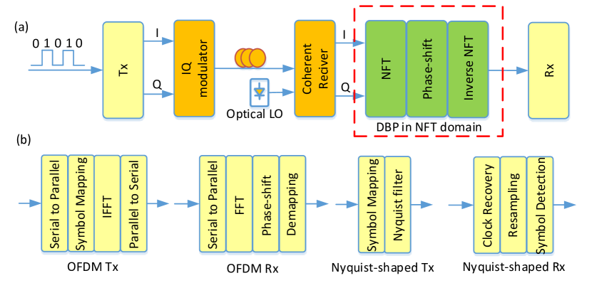
Figure 2: a) Simulation setup of coherent optical communication systems with DBP in the NFD, b) basic block functions of OFDM and Nyquist transceivers

In this section, the simulation setup that was used to assess the performance of DBP in the NFD is presented.

The transmission link was assumed to be lossless due to ideal Raman amplification, with an amplified spontaneous emission (ASE) noise density $N_{\text{ASE}}=\Gamma Lhf_{s}K_{T}$. Here, $\Gamma$ is the fiber loss, $L$ is the transmission distance, $hf_{s}$ is the photon energy, $f_{s}$ is the optical frequency of the Raman pump providing the distributed gain, and $K_{T}=1.13$ is the photon occupancy factor for Raman amplification of a fiber-optic communication system at room temperature. In the simulations, it was assumed that the long-haul fiber link consisted of $80$-km spans of fiber (standard single-mode fiber (SSMF) in the anomalous case) with a loss of $0.2$ dB/km, nonlinearity coefficient of $1.22$ W/km, and a dispersion of $\pm 16$ ps/nm/km (normal and anomalous dispersions). A photon occupancy factor of $4$ was used for more realistic conditions. The ASE noise was added after each fiber span.

The data was modulated using high spectral efficiency modulation formats (QPSK and 64QAM) and either Nyquist pulses (i.e. $\operatorname{sinc}$’s) [8] or orthogonal frequency division multiplexing (OFDM) [6, 7, 8]. The block diagram of the simulation setup and basic block functions of the OFDM and Nyquist transceivers are presented in Fig. 2. In Fig. 2(a), DBP in the NFD is performed at the receiver after coherent detection, synchronization, windowing and frequency offset compensation. For simplicity, both perfect synchronization and frequency offset compensation were assumed. The net data rates of the considered transmission systems were, after removing $7\%$ overhead due to the forward error correction (FEC), $100$ Gb/s and $300$ Gb/s for QPSK and 64QAM, respectively. For the OFDM system, the size of the inverse fast Fourier transform (IFFT) was $128$ samples, and $112$ subcarriers were filled with data using Gray coding. The remaining subcarriers were set to zero. The useful OFDM symbol duration was $2$ ns and no cyclic prefix was used for the linear dispersion removal. An oversampling factor of $8$ was adopted resulting in a total simulation bandwidth of ~$448$GHz. At the receiver side, all digital signal processing operations were performed with the same sampling rate. The receiver’s bandwidth is assumed to be unlimited in order to estimate the achievable gain offered by the proposed DBP algorithm.

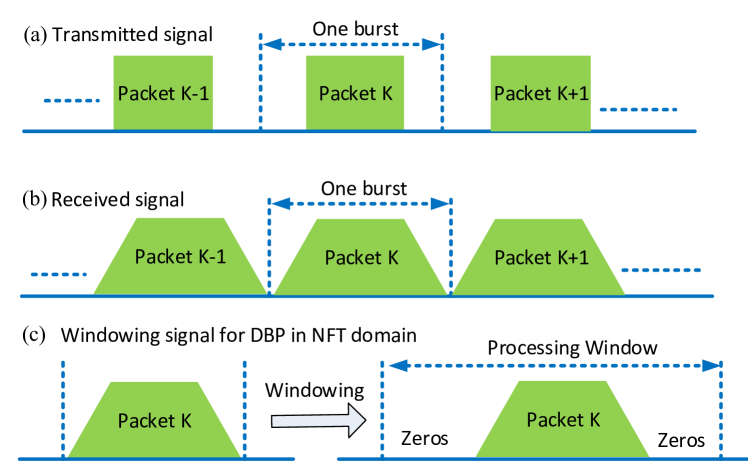
Figure 3: a) Illustration of a burst mode transmission at the transmitter side, in which neighboring packets are separated by a guard time, b) received signal at the receiver, which is broadened by chromatic dispersion, c) windowing signal for processing in the proposed nonlinear compensation scheme.

The data was transmitted in a burst mode where data packets where separated by a guard time. See Fig. 3 for an illustration. The guard time was chosen longer than the memory $\Delta T=2\pi B\beta_{2}L$ induced by the fiber chromatic dispersion (CD), where $B$ is the signal’s bandwidth, $\beta_{2}$ is the chromatic dispersion and $L$ is the transmission distance. One burst consisted of one data packet and the associated guard interval. At the receiver, after synchronization, each burst is extracted and processed separately. Since the forward and inverse NFTs require that the signal has vanished early enough before it reaches the boundaries, zero padding was applied to enlarge the processing window as in Fig. 3(c).

IV Simulation Results

In this section, the performance of DBP in the NFD is compared with a traditional DBP algorithm based on the split-step Fourier method [18] as well as with simple chromatic dispersion compensation; the latter works well only in the low-power regime where nonlinear effects are negligible.

IV-A Normal dispersion

In the normal dispersion case, a $56$ Gbaud Nyquist-shaped transmission scheme is considered in burst mode with $256$ symbols in each packet. The duration of each packet is ~$4.6$ns. The burst size is $16000$ samples and the processing window size for each burst after zero padding is $D=65536$ samples. The guard time is ~$10\%$ longer than the fiber chromatic dispersion induced memory of the link. The forward propagation is simulated using the split-step Fourier method [18] with $80$ steps/span, i.e. $1$km step. Monte-Carlo simulations were performed to estimate the system performance using the error vector magnitude (EVM) [23, (5)]. For convenience, the EVM is then converted into the $Q$-factor $20\log(\sqrt{2}\operatorname{erfc}^{-1}(2\operatorname{BER}))$ using the bit error rate (BER) estimate [23, (13)].

The performance of the $100$-Gb/s QPSK Nyquist-shaped system is depicted in Fig. 4 as a function of the launch power in a 4000km link for various configurations. An exemplary fiber in- and output as well as the corresponding reconstructed input (via DBP in the NFD) are shown in Fig. 5. It can be seen in Fig. 4 that the proposed DBP in the NFD provides a significant performance gain of ~$8.6$ dB, which is comparable with the traditional DBP employing $20$ steps/span. Traditional DBP with 40 steps/span can be considered as ideal DBP in this experiment because a further increase of the number of steps/span did not improve the performance further. In the considered $4000$km link, $40$ steps/span DBP requires $M=2000$ steps in total. This illustrates the advantage of the proposed DBP algorithm whose complexity is in contrast independent of the transmission distance. The performance of DBP in the NFD was however found to degrade rapidly when the launch power is sufficiently high. We believe that this effect can be mitigated through an extension of the processing window at the cost of increased computational complexity.

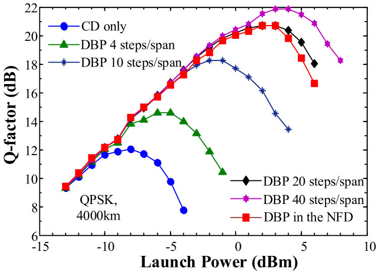
Figure 4: Performance of 100-Gb/s QPSK Nyquist-shaping over 4000km.

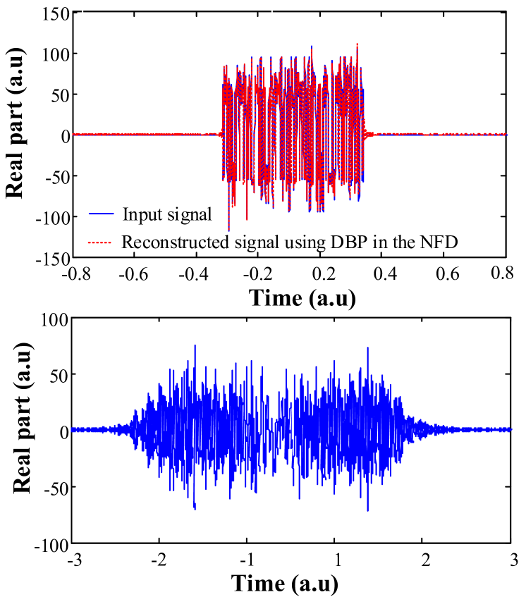
Figure 5: Top: True vs reconstructed (via DBP-NFD) fiber input for a QPSK-Nyquist signal. Bottom: Corresponding fiber output. Only real parts are shown.

A similar behavior can be observed in Fig. 6 for a $300$-Gb/s 64QAM Nyquist-shaped system. It can be seen in Fig. 6 that DBP in the NFD shows ~$1.5$ dB better performance than DBP employing $20$ steps/span. The difference from ideal DBP ($40$ steps/span) is just ~$0.6$ dB. This clearly shows that NFD-DBP can provide essentially the same performance as ideal DBP.

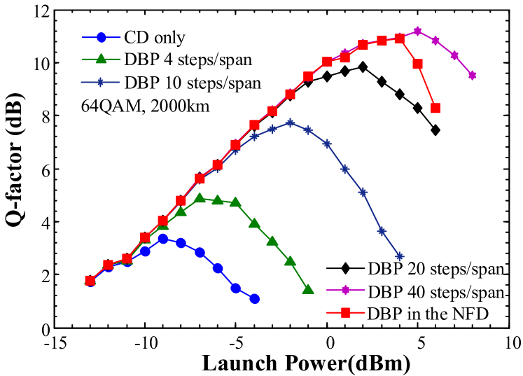
Figure 6: Performance of 300-Gb/s 64QAM Nyquit-shaping over 2000km.

IV-B Anomalous dispersion

Most fibers used today (such as SSMF) have anomalous dispersion. Therefore, it is critical to evaluate the performance of the proposed DBP algorithm in optical links with anomalous dispersion. The DBP-NFD algorithm proposed earlier however cannot yet deal with signals where the function $\alpha(0,\lambda)$ defined in (8) has roots in the upper half-plane. See Sec. II-D. The condition that the $L_{1}$-norm of each burst is less than $\pi/2$ is sufficient to ensure this condition. The packet duration in a system with anomalous dispersion thus has to be kept small enough in order to apply the proposed algorithm. This constraint is not desirable in practice, as it reduces the total throughput of the link because the guard interval, which is independent of the packet duration, must be inserted more frequently. The $L_{1}$ norm of the Fourier transform is always lower or equal to the $L_{1}$ norm of the time-domain signal. Motivated by this observation, OFDM was chosen instead of Nyquist-shaping for anomalous dispersion.

The performances of both traditional DBP and DBP in the NFD are shown in Fig. 7. DBP in the NFD can achieve a performance gain of ~$3.5$ dB, which is ~$1$ dB better than DBP employing $4$ steps/span. The performance however degrades dramatically once the launch power has become larger than $-5$dBm. We attribute this phenomenon to the emergence of upper half-plane roots of $\alpha(0,z)$, which corresponds to the formation of solitonic components in the signal. This argument is supported in Fig. 8, where the $L_{1}$-norm and the ratio between the power in the solitonic part ($\hat{E}$ in [4, p. 4320]) over the total signal power are plotted as functions of the signal power. At a launch power of $-4$ dBm, the signals begin to have solitonic components, which seems to have a significant impact on the DBP algorithm in the NFD. As anticipated in Sec. II-D, solitons indeed only occur above an $L_{1}$-norm which is significantly higher than the bound $\pi/2$.

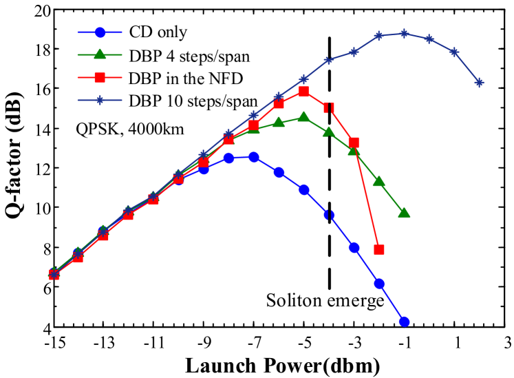
Figure 7: Performance of 100-Gb/s QPSK OFDM over 4000km in fiber with anomalous dispersion.

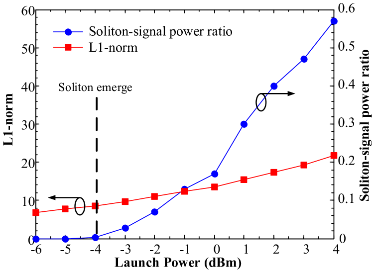
Figure 8: $L_{1}$-norm and soliton-signal power ratio for 100Gb/s OFDM.

V Conclusion

The feasibility of performing digital backpropagation in the nonlinear Fourier domain has been demonstrated with a new, fast algorithm. In simulations, this new algorithm performed very close to ideal digital backpropagation implemented with a conventional split-step Fourier method for fibers with normal dispersion at a much lower computational complexity. In the anomalous dispersion case, it was found that the algorithm works well only if the signal power is low enough such that solitonic components do not emerge. We are currently working to remove this limitation.

References

- [1] A. Hasegawa and Y. Kodama, “Guiding-center soliton in fibers with periodically varying dispersion,” Optics Lett., vol. 16, no. 18, pp. 1385–1387, 1991.
- [2] J. D. Ania-Castañón, V. Karalekas, P. Harper, and S. K. Turitsyn, “Simultaneous spatial and spectral transparency in ultralong fiber lasers,” Phys. Rev. Lett., vol. 101, 2008, 123903.
- [3] V. F. Zakharov and A. B. Shabat, “Exact theory of two-dimensional self-focusing and one-dimensional self-modulation of wave in nonlinear media,” Sov. Phys. JETP, vol. 34, no. 1, pp. 62–69, Jan. 1972.
- [4] M. I. Yousefi and F. R. Kschischang, “Information transmission using the nonlinear Fourier transform, Parts I–III,” IEEE Trans. Inf. Theory, vol. 60, no. 7, pp. 4312–4369, Jul. 2014.
- [5] E. G. Turitsyna and S. K. Turitsyn, “Digital signal processing based on inverse scattering transform,” Optics Lett., vol. 38, no. 20, pp. 4186–4188, 2013.
- [6] J. E. Prilepsky, S. A. Derevyanko, and S. K. Turitsyn, “Nonlinear spectral management: Linearization of the lossless fiber channel,” Optics Express, vol. 21, no. 20, pp. 24 344–24 367, 2013.
- [7] J. E. Prilepsky, S. A. Derevyanko, K. J. Blow, I. Gabitov, and S. K. Turitsyn, “Nonlinear inverse synthesis and eigenvalue division multiplexing in optical fiber channels,” Phys. Rev. Lett., vol. 113, Jul. 2014, article no. 013901.
- [8] S. T. Le, J. E. Prilepsky, and S. K. Turitsyn, “Nonlinear inverse synthesis for high spectral efficiency transmission in optical fibers,” Optics Express, vol. 22, no. 22, pp. 26 720–26 741, Nov. 2014.
- [9] S. Hari, F. Kschischang, and M. Yousefi, “Multi-eigenvalue communication via the nonlinear Fourier transform,” in Proc. Bien. Symp. Commun., Kingston, ON, Canada, Jun. 2014, pp. 92–95.
- [10] Q. Zhang, T. H. Chan, and A. Grant, “Spatially periodic signals for fiber channels,” in Proc. IEEE Int. Symp. Inf. Theory (ISIT), Honolulu, HI, Jun. 2014, pp. 2804–2808.
- [11] H. Bülow, “Experimental demonstration of optical signal detection using nonlinear Fourier transform,” J. Lightwave Technol., to appear, early access at http://dx.doi.org/10.1109/JLT.2015.2399014.
- [12] A. Hasegawa and T. Nyu, “Eigenvalue communication,” J. Lightwave Technol., vol. 11, no. 3, pp. 395–399, Mar. 1993.
- [13] R. Essiambre, G. Kramer, P. J. Winzer, G. J. Foschini, and B. Goebel, “Capacity limits of optical fiber networks,” J. Lightwave Technol., vol. 28, no. 4, pp. 662–701, Feb. 2010.
- [14] S. Wahls and H. V. Poor, “Introducing the fast nonlinear Fourier transform,” in Proc. IEEE Int. Conf. Acoust. Speech Signal Process. (ICASSP), Vancouver, Canada, May 2013.
- [15] ——, “Fast numerical nonlinear Fourier transforms,” Accepted for publication in IEEE Trans. Inf. Theory, Mar. 2015, arXiv:1402.1605v2.
- [16] ——, “Fast inverse nonlinear Fourier transform for generating multi-solitons in optical fiber,” IEEE Int. Symp. Inf. Theory (ISIT), Hong Kong, China, Jun. 2015, accepted for presentation, arXiv:1501.06279v1 [cs.IT].
- [17] R. Maher, T. Xu, L. Galdino, M. Sato, A. Alvarado, K. Shi, S. J. Savory, B. C. Thomsen, R. I. Killey, and P. Bayvel, “Spectrally shaped DP-16QAM super-channel transmission with multi-channel digital back-propagation,” Sci. Rep., vol. 5, Feb. 2015, article no. 8214.
- [18] E. Ip and J. M. Kahn, “Compensation of dispersion and nonlinear impairments using digital backpropagation,” J. Lightwave Technol., vol. 26, no. 20, pp. 3416–3425, Oct. 2008.
- [19] M. J. Ablowitz, D. J. Kaup, A. C. Newell, and H. Segur, “The inverse scattering transform – Fourier analysis for nonlinear problems,” Stud. Appl. Math., vol. 53, pp. 249–315, 1974.
- [20] M. Klaus and J. K. Shaw, “On the eigenvalues of Zakharov–Shabat systems,” SIAM J. Matrix Anal., vol. 34, no. 4, pp. 759–773, 2003.
- [21] S. K. Turitsyn and S. A. Derevyanko, “Soliton-based discriminator of noncoherent optical pulses,” Phys. Rev. A, vol. 78, no. 6, 2008, article no. 063819.
- [22] S. A. Derevyanko and J. E. Prilepsky, “Soliton generation from randomly modulated return-to-zero pulses,” Optics Commun., vol. 281, no. 21, pp. 5439–5443, 2008.
- [23] R. A. Shafik, M. S. Rahman, and A. H. M. R. Islam, “On the extended relationships among EVM, BER and SNR as performance metrics,” in Proc. Int. Conf. Electr. Comput. Eng. (ICECE), Bangladesh, Dec. 2006.