On the homotopy type of the Acyclic MacPhersonian
In 2003 Daniel K. Biss published, in the Annals of Mathematics [1], what he thought was a solution of a long standing problem, culminating a discovery due to Gel’fand and MacPherson [4]; namely, he claimed that the MacPhersonian —a.k.a. the matroid Grassmannian— has the same homotoy type of the Grassmannian. Six years later he was encouraged to publish an “erratum” to his proof [2], observed by Nikolai Mnëv; up to now, the homotopy type of the MacPhersonian remains a mystery…
The Acyclic MacPhersonian is to the MacPhersonian, as it is the class of all acyclic oriented matroids, of a given dimension and order , to the class of all oriented matroids, of the same dimension and order. The aim of this note is to study the homotopy type of in comparison with the Grassmannian , which consists of all linear subspaces of , with the usual topology — recall that, due to the duality given by the “orthogonal complement”, and are homeomorphic. For, we will define a series of spaces, and maps between them, which we summarise in the following diagram:
In this diagram, the maps labeled represents inclusions and those labeled are natural projections; the compositions of these will prove homotopical equivalences. The main function is which retracts the fat acyclic MacPhersonian —to be defined— to the (Affine) Grassmannian ; this will be study through the mean curvature flow defined in the elements of , the space of all spherical Radon separoids of dimension and order — see [12] for a compact introduction to separoid theory. A recent result of Zhao et al. (2018) allow us to prove that this flow “stretches” wiggled spheres, representing acyclic oriented matroids, onto geodesic spheres, representing affine configurations of points (cf. [6, 7]).
1 Preliminaries
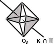
We will represent the elements of all our spaces as “spherical” subspaces of the -octahedron of radius 2 in :
It is the combinatorial structure of these hyper-octahedra —or cross polytopes if you will— that allow us to encode the circuits of the oriented matroids we will be dealing with. The reader is encouraged to read [5, 8, 9] to better understand this approach; however, in order to be self-contained, we start by working out a simple example to have in mind during the rest of the exposition:
Consider a configuration of 4 points in the real line, say on the numbers (points) and . From the affine point of view (modulus the affine group), this configuration is equivalent to the one on the numbers and , but different from that on the numbers and . The configuration can be encoded with the matrix which represents a linear function . The minimal Radon partitions of this configuration are , , and ; these are the circuits of the associated oriented matroid. Here, and in the sequel, we denote by the symmetric relation the fact that two subsets are disjoin but their convex hull do intersect (cf. [10]); that is,
Observe that, from the combinatorial point of view, the three configurations exemplified above define the same oriented matroid, while the affine group distinguish the last from the other two.
The Radon partitions of the configuration can be deduced from the solutions, in , to the following three equations:
where the denote the points of the configuration.
For example, from the solution we deduce that .
Observe that the space of solutions is the intersection of three easy described spaces; namely, the kernel of the linear function, the hyperplane orthogonal to the vector , and the -octahedron. Since the kernel is a flat of dimension 3, the hyperplane is also of dimension 3, and the -octahedron is an sphere of dimension 3, then is homeomorphic to the sphere of dimension 1.
Conversely, given a geodesic 1-dimensional sphere contained in , we can extend it to a 3-dimensional subspace, not contained in , which is the kernel of a linear function encoding a configuration of 4 points in the line. That is to say, all configurations of 4 points in the line are in 1-to-1 relation with the family of geodesic 1-dimensional spheres inside . Analogously, we can identify the configuration of 4 points in the line with the 2-subspaces of ; therefore, the configurations of 4 points in the line are in 1-to-1 relation with the points of the Grassmannian of 2-subspaces of , the projective plane.
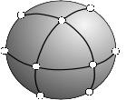
Back to our example , we can observe that inherits from the combinatorial structure of a cycle of length 8; namely, its vertices arise from the minimal Radon partitions, and its antipodes, and the edges are the arcs that join these vertices along the circle . Indeed, this is the so-called circuit graph of the associated oriented matroid (see [9]). However, if we are given just the labeled circuit graph of the oriented matroid, there is no canonic way to choose a single circle to represent it; in particular, there is no way to choose the configuration on the points and or the one on the points and . We solve this “anomaly” by choosing a “wiggled” but canonic circle, namely we take the baricentres of each face of representing the corresponding circuit; that is, we take the points , with its antipodes, and connect them with geodesic arcs in the obvious way.
We can go one step further and consider “all those wiggled circles” contained in such that its vertices are the circuits of an acyclic oriented matroid —this is what I call the fat acyclic MacPhersonian .
In a similar way, we can represent the acyclic MacPhersonian with “some wiggled circles” contained in ; namely, for each acyclic oriented matroid, we take that “circle” whose vertices are in the baricentres of the respective faces of , and each simplex of —each chain in the partial order of specialisation— is closed taking the “convex closure” in the space . Since each face of is contractible, the natural map
has contractible fibbers, and therefore it is a homotopical equivalence.
Finally, we can apply to each circle of a heat-type flow (we will use in the general case the mean curvature flow; see [6, 7]) to stretch it and ending up with an element of . This exhibits a strong retraction showing that , and therefore , have the homotopy type of the projective plane. In the appendix it can be fund a Python code that exhibits an implementation of such a flow for this case.
1.1 The Affine Grassmannian
Given points in dimension , we can build a matrix consisting of these column vectors. This matrix is naturally identified with the linear map which sends the cannonical base of onto the points, and two such functions are affinely equivalent if, and only if, their respective kernels intersect the hyperplane
in exactly the same subspace (cf. [8]): .
If the points span the -dimentional space, the kernel of such a function is of dimention , and we can identify the configuration with the subspace of the hyperplane ; thus, we can identify each configuration with a point of the Grassmannian which consists of all planes of , with the usual topology.
Furthermore, the intersection of each such a plane with the -octahedron define the Radon complex of the configuration; it is a CW-complex which is an -sphere (see [8]), whose 1-skeleton is the so-called circuit graph of the corresponding oriented matroid — or the cocircuit graph of its dual, if you will. The cocircuit graphs of oriented oriented matroids where characterised in [5, 9].
Observe that corresponds to the space of all configurations of points in dimension , modulus the affine group; it is the double cover of , which is homeomorphic to the -projective space.
We further endow with a partition; namely, we relate two elements of if their corresponding configurations represent the same oriented matroid; the realisation space of the configuration is the set of all those that represent the same (lebeled) oriented matroid (cf. [3] ch. 8). In particular, each realisation space in is contractible; for, observe that an affine configuration of points in is determined by a unique Radon partition (a unique circuit) , and its realisation space is then a cell which can be parametrised with the points of , where represents the simplex of rank (see Figure 2).
1.2 The Acyclic MacPhersonian
The family of all oriented matroids on elements in dimension can be partially ordered by specialisation; viz., we say that if every minimal Radon partition of is a Radon partition of . Given such a partial order, we can define the topological space of its chains, in the usual way, and if we considere only acyclic oriented matroids (of elements in dimension ) we get the acyclic MacPhersonian .
For example, consider all acyclic oriented matroids arising from 4 points spanning the affine plane; i.e., those acyclic oriented matroids whose circuits are the Radon partitions of 4 points in . There are 3 labeled configurations in general position with the four points in the boundary of the convex hull, and 4 configurations where one of them is in the interior of the convex hull of the other three. These 7 uniform oriented matroids can be represented by 3 squares and 4 triangles that, when joining them together, form the hemicuboctahedron. The boundaries of these 7 “discs” represents those configurations which are not in general position (non-uniform acyclic oriented matroids); there are 12 edges coming from those where one element is in the interior of the segment of other two, and 6 vertices representing those where two points coincide —this is exactly after identifying antipodes. That is to say, is homeomorphic to ; indeed, is the first baricentric subdivision of endowed with the partition described below.
1.3 The space of Spherical Radon Separoids
A separoid is a set endowed with a symmetric relation on disjoin subsets of (i.e., ), closed as a filter; that is,
A related pair is called a Radon partition, and it is enough to know the minimal Radon partitions of a separoid to reconstruct it. The order of the separoid is the cardinal of its base set and its dimension is the minimum that makes Radon’s lemma true; that is,
We say that the separoid is in general position if every minimal Radon partition consist of elements. Two disjoint subsets which are not related (are not a Radon partition) are separated and we denote .
The separoid is acyclic if the empty set is separated from the base set ; in other words, if no Radon partition involves the empty set:
All acyclic separoids can be represented with families of convex polytopes in and their separations by affine hyperplanes (cf. [BS]).
A Radon separoid is a separoid whose minimal Radon partition are unique on their supports; namely, if and are minimal Radon partitions, then
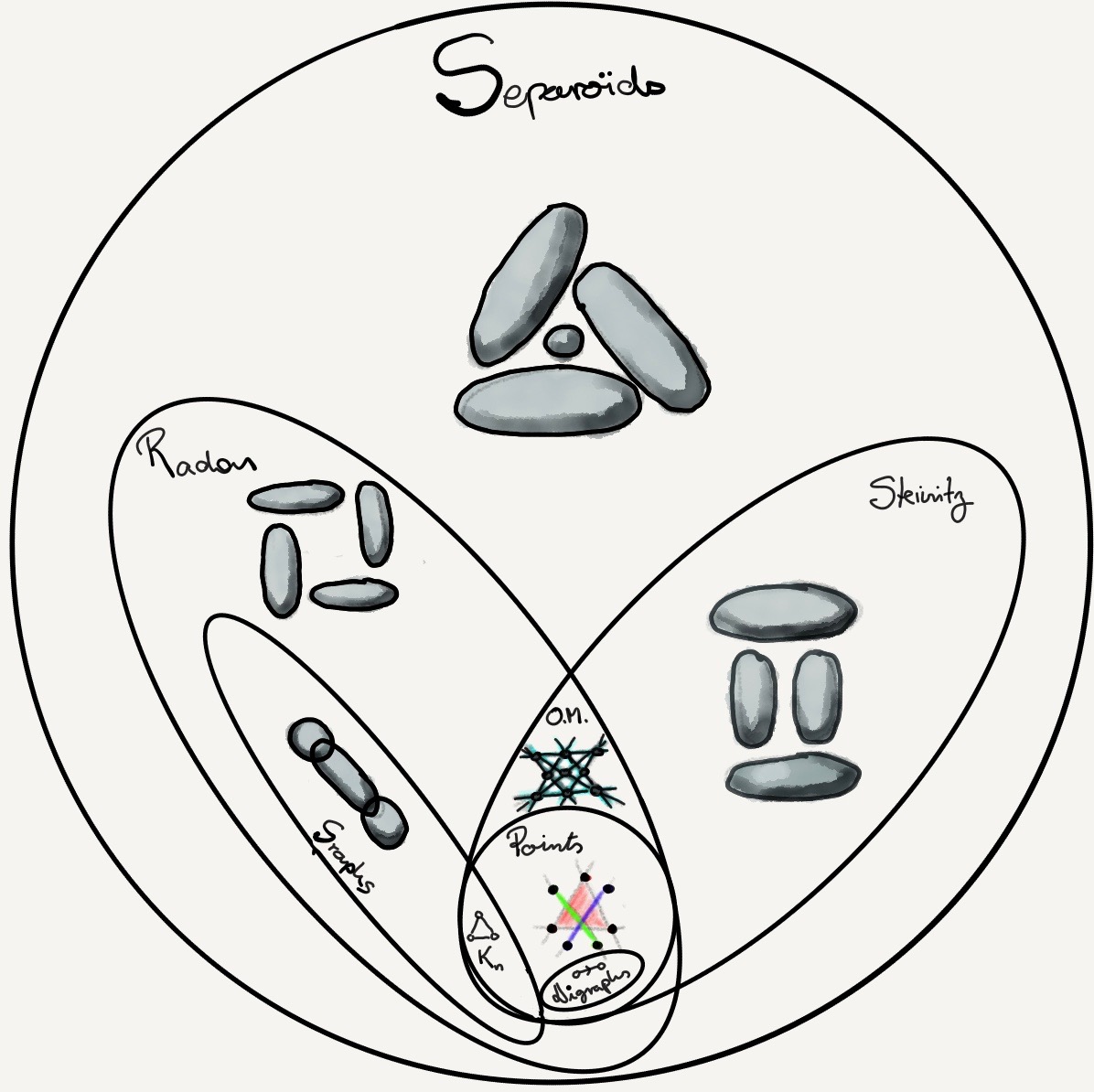
The minimal Radon partitions of a Radon separoid are the circuits of an oriented matroid if they satisfy the so-called week elimination axiom: if and are minimal Radon partitions, then
Oriented matroids are Steinitz separoids (cf. [LV]); that is, their minimal Radon partitions satisfies the so-called Steinitz exchange axiom for circuits: if is minimal and ,
This property induces a cyclic order in the minimal Radon partitions of uniform oriented matroids of order , and therefore their Radon complex (to be defined below) is a cycle —see [8] for another application of this fact.
1.3.1 The Radon complex of a separoid
Consider the -cube and identify its vertices with the subsets of the -set , in the usual way. Through this identification, it is easy to see that the faces of are the intervals in the natural partial order induced by the inclusion. Since the -octahedron is the dual polytope of , its faces can be labeled with such intervals too.
Given a separoid , we will assign a subcomplex of made out of those faces where is a Radon partition and denotes the complement; is called the Radon complex of (cf. [8]).
We say that a separoid is spherical if its Radon complex is a sphere. In particular, oriented matroids are spherical Radon separoids.
2 Stretching spheres
To understand the acyclic MacPhersonian, we first identify each acyclic oriented matroid with its set of circuits. They are encoded in the vertices of the circuit graph, which is well know to be the 1-skeleton of a -sphere; indeed, we start with such a “wiggled sphere” and applying to it the mean curvature flow to stretch it, we end up with a “geodesical sphere” which represents an affine configuration of points. This way, we can assign to each acyclic oriented matroid an affine configuration of points, and in such a way that we are defining a homotopical retraction from the acyclic MacPhersonian to the affine Grassmannian.
2.1 Oriented Matroids as spheres inside .
In [9] we characterised the circuit graphs of oriented matroids as those graphs which can be embedded in what we called “the -dual of the -cube”, with some extra properties… that was to say that its vertices can be labeled with the faces of
We will identify such circuits (and the corresponding vertices in the circuit graph) with the barycentre of such faces. The vertices of are points of the form
where and in the th element of the canonical base of ; and each face of it can be determined in terms of the convex hull of the vertices that it contain. Therefore, each circuit of a given oriented matroid can (and will) be coordinatised in terms of differences of the canonical base vectors of :
If we “fill up the faces” of the circuit graph, considering all its vectors, we end up with a PL-complex which is well known to be an sphere of dimension ; that is, we can identify each oriented matroid on elements in dimension with a, not necesarly “flat”, ()-sphere inside . An oriented matroid is stretchable if and only if there is a flat ()-sphere inside whose 1-skeleton is the circuit graph (cf., [8]).
2.2 The “fat” MacPhersonian
We now consider a space which is much more “fatty” than the acyclic MacPhersonian and the affine Grassmannian, but contains both of them:
That is, we take several copies of each sphere representing an oriented matroid, while considering all possible embeddings of such a sphere inside its natural ambiance space , with the extra freedom of having its vertices in any point representig the corresponding circuit (not only the baricentre of it).
Clearly, since all faces of are contractible, and have the same homotopy type, and is embedded in as it is in (recall the diagram in the first page of this note).
It remains to show that is a homotopical retract of .
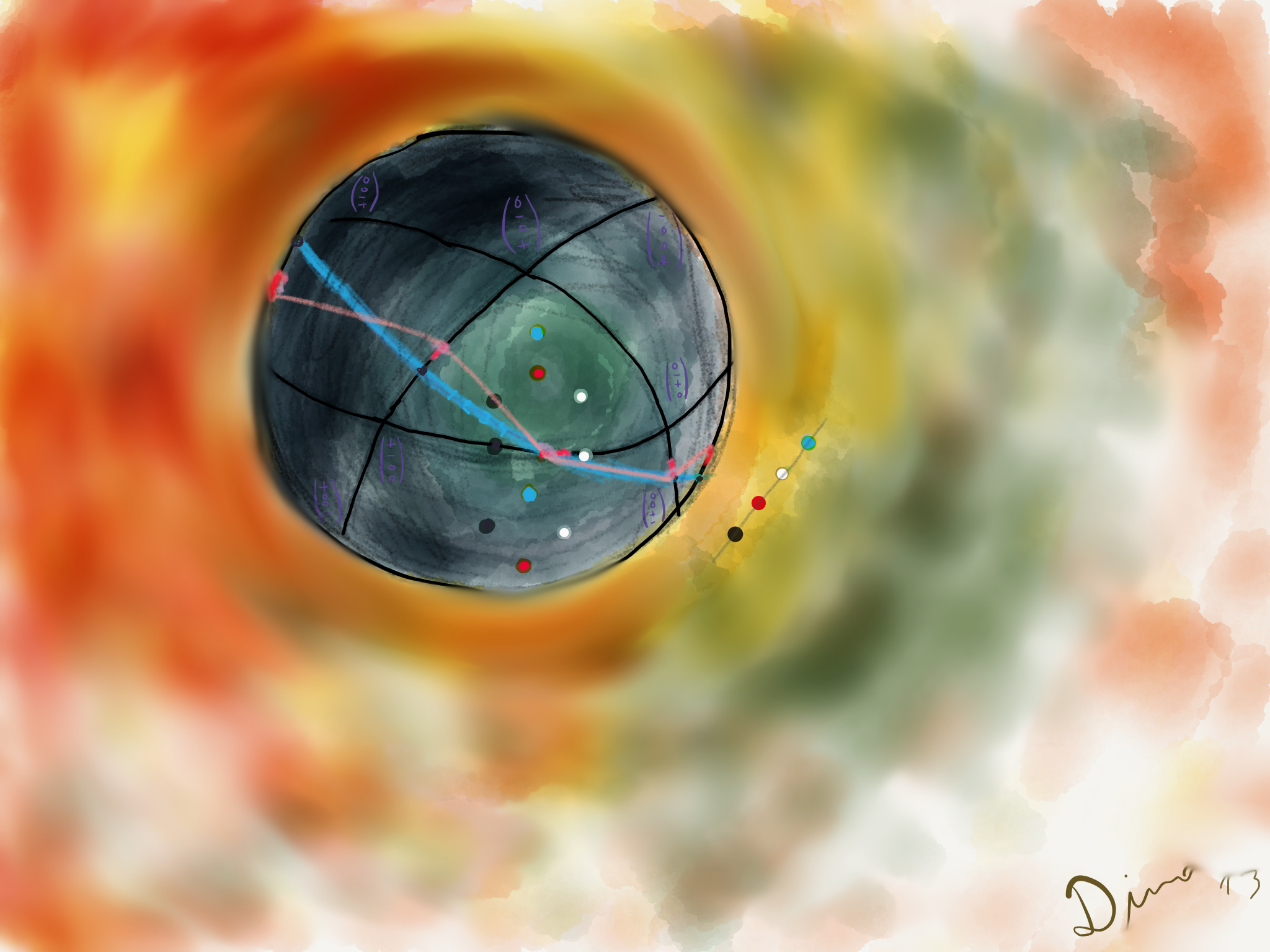
2.3 Mean Curvature Flow on
We need now to use some tools of differential geometry, so we need to “soft” our PL-spaces; for, we just change the PL-sphere by an euclidian sphere, but keeping the partition of such a sphere given by the faces of the octahedron. That is, in this section by we will denote the sphere of radius 2 endowed with the partition induced by the intersection with the canonical subspaces of , those generated by positive cones of the canonical base, and its negatives. So, we have the vertices given by the 1-dimensional subspaces spanned by the canonic vectors ; the edges between them are geodesic segments contained in the intersection of the 2-dimensional subspaces spanned by pairs of canonic vectors; geodesic triangles are the intersection of the positive cone of three independent canonic vectors, or its negatives; and so on… So, we preserve the combinatorics imposed by the octahedron, but our ambience space is now the differentiable euclidian sphere instead.
Analogously, when we consider an element of the “fat” MacPhersonian, a “wiggly” -sphere whose vertices lie on the “smoothed” faces of , we consider its embedding to be differentiable. That is, for each element we have a smooth immersion of an -sphere into the -sphere , endowed with the combinatorial decomposition induced by the -octahedron. The one parameter family of immersions satisfying
where denotes the normal component of and denotes the mean curvature vector of , is known as the mean curvature flow with initial value .
It can be proved that, if and then converges uniformly to a geodesic sphere , which represents a configuration of points in the -dimensional affine space. More generally, if is the Radon complex of a spherical Radon separoid, then the limit is a geodesic sphere; observe that for all we have that , therefore is a strong retraction of .
It remains to prove that, if then for all we have that .
References
- [1] Biss, Daniel K.; The homotopy type of the matroid Grassmannian. Ann. Math. (2) 158, No. 3, 929-952 (2003).
- [2] Biss, Daniel K.; Erratum to “The homotopy type of the matroid Grassmannian”. Annals of Mathematics, 170 (2009), p. 493.
- [3] Bjorner et al.; Oriented Matroids; Cambridge University Press (1993).
- [4] Gelfand, I.M.; MacPherson, Robert D.; A combinatorial formula for the Pontrjagin classes. Bull. Am. Math. Soc., New Ser. 26, No.2, 304-309 (1992).
- [5] Knauer, Kolja; Montellano-Ballesteros, Juan José; Strausz, Ricardo; A graph-theoretical axiomatization of oriented matroids. Eur. J. Comb. 35, 388-391 (2014).
- [6] Liu, Kefeng; Xu, Hongwei; and Zhao, Entao; Deforming submanifolds of arbitrary codimension in a sphere. arXiv:1204.0106v1 (2012).
- [7] Liu, Kefeng; Xu, Hongwei; Fei Ye; Zhao, Entao; THE EXTENSION AND CONVERGENCE OF MEAN CURVATURE FLOW IN HIGHER CODIMENSION. TRANSACTIONS OF THE AMERICAN MATHEMATICAL SOCIETY. Volume 370, Number 3, March 2018, Pages 2231–2262.
- [8] Montellano-Ballesteros, Juan José; Strausz, Ricardo; Counting polytopes via the Radon complex. J. Comb. Theory, Ser. A 106, No. 1, 109-121 (2004).
- [9] Montellano-Ballesteros, Juan José; Strausz, Ricardo; A characterization of cocircuit graphs of uniform oriented matroids. J. Comb. Theory, Ser. B 96, No. 4, 445-454 (2006).
- [10] Nešetřil, Jaroslav; Strausz, Ricardo; Universality of separoids. Arch. Math., Brno 42, No. 1, 85-101 (2006).
- [11] Shor, Peter W.; Stretchability of pseudolines is NP-hard. Applied geometry and discrete mathematics, Festschr. 65th Birthday Victor Klee, DIMACS, Ser. Discret. Math. Theor. Comput. Sci. 4, 531-554 (1991).
- [12] Strausz, Ricardo; Erdős-Szekeres “happy end”-type theorems for separoïds. Eur. J. Comb. 29, 1076-1085 (2008).