Transmission through correlated Cu_nCoCu_n heterostructures

Abstract

The effects of local electronic interactions and finite temperatures upon the transmission across the Cu₄CoCu₄ metallic heterostructure are studied in a combined density functional and dynamical mean field theory. It is shown that, as the electronic correlations are taken into account via a local but dynamic self-energy, the total transmission at the Fermi level gets reduced (predominantly in the minority spin channel), whereby the spin polarization of the transmission increases. The latter is due to a more significant $d$-electrons contribution, as compared to the non-correlated case in which the transport is dominated by $s$ and $p$ electrons.

I Introduction

The design of multi-layered heterostructures composed of alternating magnetic and non-magnetic metals offers large flexibility in tailoring spin-sensitive electron transport properties of devices in which the current flow is perpendicular to the planes. In the framework of ballistic transport, the spin-polarized conductance and the giant magnetoresistance effect (GMR) depends on the mismatch between the electronic bands of the concerned metals near the Fermi level [1, 2]. In order to maximize the spin polarization of current and hence the GMR, heterostructures including half-metallic materials [3, 4, 5] seem to be the materials of choice. In practice, however, the spin-polarization is never complete due to the presence of defects, and/or due to intrinsic limitations caused by spin-contamination and spin-orbit coupling [5]. Owing to the technological relevance, considerable progress has been achieved in the computational description of multilayered heterostructures. In particular, the ballistic transport properties have been addressed by considering the Landauer-Büttiker formalism [6, 7, 8, 9], where the conductance is determined by the electron transmission probability through the device region, which is placed between two semi-infinite electrodes. The transmission probability can be then computed with different electronic structure approaches, such as the tight-binding [10, 11, 12, 13] or the first-principles density functional theory (DFT) ones [14, 15, 16]. Various implementations exist, based on transfer matrix [17, 18], layer-Korringa–Kohn–Rostoker (KKR) [19, 20], or non-equilibrium Green’s function (NEGF) [21] techniques.

In the context of first-principles calculations, it is known that, for systems with moderate to strong electron correlations, the electronic structure, calculated with the “conventional” DFT local density approximation (LDA) or its generalized gradient approximation (GGA) extension, is not accurate enough to account for the observed spectroscopic behavior. A more adequate description is provided within the dynamical mean field theory (DMFT) [22, 23, 24] built on the LDA framework [25, 26, 27]. Since many interesting magnetic materials fall into this category, the prediction of their electron transport properties, obtained by combining the Landauer-Büttiker formalism with DFT [21, 28, 29], is expected to equally suffer from an insufficient treatement of correlation effects, which would be captured by adding DMFT. However, the full incorporation of correlation effects at the DMFT level into the transport calculations is not straightforward, not only because of technical reasons, such as large system size and lack of corresponding algorithms, but also because of conceptual difficulties in the development of many-body solvers in the out-of-equilibrium regime [30]. Attempts to close this gap include the use of combined techniques, in which equilibrium-DMFT calculations are performed in order to obtain the Landauer conductance of atomic contacts made of transition metals [31, 32].

In this work, we investigate the linear-response transport through a prototypical Cu-Co-Cu heterostructure by accounting for strong electron correlation effects in the electronic structure of the Co monolayer. The attention to this system is drawn by a significant density of states that develops in the Co layer, in the vicinity of the Fermi level, in one spin channel only (the minority-spin one), whereas the Cu layers contribute with states at higher binding energies. We use a “two-step” approach, in which the Landauer transmission probability is calculated within the smeagol NEGF based electron transport code [21, 28, 29] whereby the Hamiltonian is obtained from DFT [33]. The many-body corrections to the Green’s function are evaluated using DMFT in an exact muffin-tin orbitals (EMTO)-based package [34, 35, 36], which uses a screened KKR approach [37]. These corrections are then passed to smeagol for the calculation of the transport properties.

The article is organized as follows. We start with a general description of the transport problem in the presence of electronic correlations (Sec. II.1). Then the computational details are outlined in Sec. II.2, and the geometry of the system considered in our simulations is descried in Sec. II.3. Finally, Sec. III presents the main results, and Sec. IV summarizes and concludes. The appendices deal with technical implementation and various tests, notably App. B explains porting the results from EMTO into smeagol, and discusses a model two-orbital system of cubic symmetry.

II Methods

II.1 Transport properties in the presence of electronic correlations

The electronic transport through a device can be addressed using the Kubo approach, where the central quantity is the conductivity, and the electrical current is the result of the linear response of the system to an applied electric field [38]. Alternatively, in the Landauer-Büttiker formulation [6, 7, 8, 9], the current flow through a device is considered as a transmission process across a finite-sized scattering region placed between two semi-infinite leads, connected at infinity to charge reservoirs. The quantity of interest is the conductance, which, within linear response, is given by:

$$\mathcal{G}=\frac{e^{2}}{h}\frac{1}{\Omega_{\mathrm{BZ}}}\sum_{\sigma=\uparrow,\downarrow}\int_{\mathrm{BZ}}\!d\mathbf{k}_{\parallel}T_{\sigma}(\mathbf{k}_{\parallel},E_{F}),$$ (1)

where $-e$ is the electron charge, $h$ the Planck constant, and $e^{2}/h$ half the quantum of conductance. $T_{\sigma}(\mathbf{k}_{\parallel},E_{F})$ is the spin-dependent transmission probability from one lead to the other for electrons at the Fermi energy and with the transverse wave-vector $\mathbf{k}_{\parallel}$ perpendicular to the current flow (here we assume that the two spin-components do not mix). The integral over $\mathbf{k}_{\parallel}$ goes over the Brillouin zone (BZ) perpendicular to the transport direction, and $\Omega_{\mathrm{BZ}}$ is the area of the BZ. In the case when the interaction between electrons involved in transport is completely neglected, the transmission for a given energy, $E$, of the incident electrons can be evaluated as [39]

$$T_{\sigma}(\mathbf{k}_{\parallel},E)={\rm Tr}\left[\mathbf{\Gamma}_{L}^{\sigma}(\mathbf{k}_{\parallel},E)\mathbf{G}^{\sigma\dagger}(\mathbf{k}_{\parallel},E)\mathbf{\Gamma}_{R}^{\sigma}(\mathbf{k}_{\parallel},E)\mathbf{G}^{\sigma}(\mathbf{k}_{\parallel},E)\right],$$ (2)

where $\mathbf{G}^{\sigma}(\mathbf{k}_{\parallel},E)$ is the retarded Green’s function of the scattering region coupled to the leads,

$$\mathbf{G}^{\sigma}(\mathbf{k}_{\parallel},E)=\left[\epsilon^{+}\mathbf{S}(\mathbf{k}_{\parallel})-\mathbf{H}^{\sigma}(\mathbf{k}_{\parallel})-\mathbf{\Sigma}_{L}^{\sigma}(\mathbf{k}_{\parallel},E)-\mathbf{\Sigma}_{R}^{\sigma}(\mathbf{k}_{\parallel},E)\right]^{-1}.$$ (3)

All terms presented are matrices $[\mathbf{G}^{\sigma}(\mathbf{k}_{\parallel},E)]_{\mu\nu}$, labelled by the global indices $\mu$, $\nu$ which run through the basis functions at all atomic positions in the scattering region. $\mathbf{S}(\mathbf{k}_{\parallel})$ represents the orbital overlap matrix, and the energy shift into the complex plane, $\epsilon^{+}=\lim_{\delta\to 0^{+}}(E+i\delta)$, has been introduced to respect causality. $\mathbf{H}^{\sigma}(\mathbf{k}_{\parallel})$ is the Hamiltonian of the scattering region for spin $\sigma$; the right and left self-energies $\mathbf{\Sigma}_{R}^{\sigma}(\mathbf{k}_{\parallel},E)$ and $\mathbf{\Sigma}_{L}^{\sigma}(\mathbf{k}_{\parallel},E)$ describe the energy-, momentum- and spin-dependent hybridization of the scattering region with the left and right leads, respectively [29]. Therefore, $\mathbf{G}^{\sigma}(\mathbf{k}_{\parallel},E)$ is formally the retarded Green function associated to the effective, non-hermitian Hamiltonian $\mathbf{H}^{\sigma}_{\rm eff}(\mathbf{k}_{\parallel},E)=\mathbf{H}^{\sigma}(\mathbf{k}_{\parallel})-\mathbf{\Sigma}_{L}^{\mathbf{\sigma}}(\mathbf{k}_{\parallel},E)-\mathbf{\Sigma}_{R}^{\sigma}(\mathbf{k}_{\parallel},E)$, in which the self-energies act as external energy-, momentum- and spin-dependent potentials. In Eq. (2), $\mathbf{\Gamma}_{L(R)}^{\mathbf{\sigma}}(\mathbf{k}_{\parallel},E)=i\big{[}\mathbf{\Sigma}_{L(R)}^{\sigma}(\mathbf{k}_{\parallel},E)-\mathbf{\Sigma}_{L(R)}^{\sigma\dagger}(\mathbf{k}_{\parallel},E)\big{]}$ is the so-called left (right) broadening matrix that accounts for the hybridization-induced broadening of the single-particle energy levels of the scattering region. Importantly, for non-interacting electrons, it has been proved that the Landauer and the Kubo approaches are equivalent [40], so that the linear-response transport properties of a system can be computed with either formalism. During the last few years, the Landauer approach has been systematically applied in conjunction with DFT in order to perform calculations of the conductance of different classes of real nano-devices [41]. In this combination the DFT provides a single-particle theory in which the Kohn-Sham eigenstates are interpreted as single-particle excitations. Although this approach is only valid approximatively, DFT-based transport studies have provided insightful results concerning the role of the band-structure in the electron transport process through layered heterostructures [1, 2, 42, 43, 44].

With the effect of the electron-electron interaction beyond the DFT explicitly considered, the retarded Green’s function of Eq. (3) is replaced by the following one, carrying the subscript “MB” for “many-body”:

$$\mathbf{G}^{\sigma}_{MB}(\mathbf{k}_{\parallel},E)=\left[\epsilon^{+}\mathbf{S}(\mathbf{k}_{\parallel})-\mathbf{H}^{\sigma}(\mathbf{k}_{\parallel})-\mathbf{\Sigma}_{L}^{\sigma}(\mathbf{k}_{\parallel},E)-\mathbf{\Sigma}_{R}^{\sigma}(\mathbf{k}_{\parallel},E)-\mathbf{\Sigma}_{MB}^{\sigma}(\mathbf{k}_{\parallel},E)\right]^{-1}.$$ (4)

Here, $\mathbf{\Sigma}^{\sigma}_{MB}(\mathbf{k}_{\parallel},E)$ is the many-body self-energy defined through the Dyson equation $\mathbf{\Sigma}^{\sigma}_{MB}(\mathbf{k}_{\parallel},E)=\mathbf{G}^{\sigma}(\mathbf{k}_{\parallel},E)^{-1}-\mathbf{G}^{\sigma}_{MB}(\mathbf{k}_{\parallel},E)^{-1}$ [38]. This accounts for all electron-electron interaction effects neglected in $\mathbf{G}^{\sigma}(\mathbf{k}_{\parallel},E)$. The self-energy acts as a spin-, momentum- and energy-dependent potential, whose imaginary part produces a broadening of the single-particle states due to finite electron-electron lifetime. In this work, the many-body self-energy is computed at the DMFT level, meaning that $\mathbf{\Sigma}^{\sigma}_{MB}(\mathbf{k}_{\parallel},E)$ is approximated by a ${\bf k}$-independent quantity $\mathbf{\Sigma}^{\sigma}_{MB}(E)$, i.e., a spatially local but energy-dependent potential. Then, as suggested by Jacob et al.  [31, 32], the conductance and the transmission probability are obtained within the Landauer approach by using Eqs. (1) and (2), where one replaces $\mathbf{G}^{\sigma}(\mathbf{k}_{\parallel},E)$ by $\mathbf{G}_{\mathrm{MB}}^{\sigma}(\mathbf{k}_{\parallel},E)$. This is an approximation, since it neglects vertex corrections due to in-scattering processes [45, 46], which in general increases the conductivity. But we are not aware of any established method to compute those vertex corrections to linear-response transport within the considered framework. In our approach the Landauer transmission is calculated using the improved DMFT electronic structure, rather than the DFT one. Note that the DMFT provides the single-particle excitations of the system, whereas the Kohn-Sham DFT eigenvalues formally do not reveal such quasiparticle states.

II.2 DMFT-based computational approach

The transport calculations are performed according to the Green’s function scheme presented above by using the DFT-based transport code smeagol [28, 21, 29]. The many-body self-energy entering in Eq. (4) is calculated using the EMTO-DMFT method [47, 34, 35, 36] within a screened KKR [37] approach. In both codes the Perdew-Burke-Ernzerhof (PBE) GGA [48] for the exchange-correlation density functional is used. Self-consistent DFT calculations are performed separately in smeagol and in the EMTO-code. The many-body self-energy is then evaluated after self-consistency in the EMTO-code, and passed to the smeagol Green’s function to compute the transmission along Eq. (2). The smeagol imports the DFT Hamiltonian from the siesta code [33], which uses pseudopotentials and expands the wave functions of valence electrons over the basis of numerical atomic orbitals (NAOs). The EMTO code, in its turn, uses the muffin-tin construction; we present a detailed description of the projection of quantities such as the many-body self-energy from the EMTO basis set into the NAO basis set (smeagol/siesta) in the Appendix.

For the EMTO-DMFT calculations, the following multi-orbital on-site interaction term is added to the GGA Hamiltonian in the EMTO basis: $\frac{1}{2}\sum_{{i\{m,\sigma\}}}U_{mm^{\prime}m^{\prime\prime}m^{\prime\prime\prime}}c^{{\dagger}}_{im\sigma}c^{{\dagger}}_{im^{\prime}\sigma^{\prime}}c_{im^{\prime\prime\prime}\sigma^{\prime}}c_{im^{\prime\prime}\sigma}$. Here, $c_{im\sigma}$($c^{\dagger}_{im\sigma}$) destroys (creates) an electron with spin $\sigma$ on orbital $m$ at the site $i$. The Coulomb matrix elements $U_{mm^{\prime}m^{\prime\prime}m^{\prime\prime\prime}}$ are expressed in the standard way [49] in terms of three Kanamori parameters $U$, $U^{\prime}$ and $J$. Then, within DMFT the many-body system is mapped onto a multi-orbital quantum impurity problem, which corresponds to a set of local degrees of freedom connected to a bath and obeys a self-consistently condition [23, 24]. In the present work the impurity problem is solved with a spin-polarized $T$-matrix fluctuation exchange (SPTF) method [26, 50]. This method was first proposed by Bickers and Scalapino [51] in the context of lattice models. In practice, it is a perturbative expansion of the self-energy in powers of $U$, with a resummation of a specific classes of diagrams, such as ring diagrams and ladder diagrams. The expansion remains reliable when the strength of interaction $U$ is smaller than the bandwidth of the bath, which is fulfilled in the case of Cu-Co-Cu heterostructures and for the considered values of the Coulomb parameters. The impurity solver we use is multi-orbital, fully rotationally invariant, and moreover computationally fast, since it involves matrix operations like inversions and multiplications. The perturbation theory can be performed either self-consistently, in terms of the fully dressed Green’s function, or non-self-consistently, as was done in the initial implementations [47, 52]. When the interaction is small with respect to the bandwidth, no appreciable difference exists between the non-self-consistent and self-consistent results [53, 54]. This has to be distinguished from the DMFT self-consistency, which is employed in both cases. In the present calculation, we use non-dressed Green’s functions to perform these infinite summation of diagrams. Moreover, we consider a different treatment of particle-hole (PH) and particle-particle (PP) channels. The particle-particle (PP) channel is described by the $T$-matrix approach [55] which yields renormalization of the effective interaction. This effective interaction is used explicitly in the particle-hole channel; details of this scheme can be found in Ref. [50]. The particle-particle contribution to the self-energy is combined with the Hartree-Fock and the second-order contributions [56]. The many-body self-energy is computed at Matsubara frequencies $\omega_{n}=(2n+1)\pi/\beta$, where $n=0,1,2,...$ and $\beta$ is the inverse temperature. The Padé [57] analytical continuation is employed to map the self-energies from the Matsubara frequencies onto real energies, as required in the transmission calculation. Note that since some parts of the correlation effects are already included in the GGA, the double counting of some terms has to be corrected. To this end, we start with the GGA electronic structure and replace the obtained $\mathbf{\Sigma}^{\sigma}_{MB}(E)$ by $\mathbf{\Sigma}_{MB}^{\sigma}(E)-\mathbf{\Sigma}_{MB}^{\sigma}(0)$ in all equations of the GGA+DMFT method [58], the energy $E$ here being relative to the Fermi energy. This is a common double-counting correction for treating metals; a more detailed description can be found in [59].

II.3 Cu-Co-Cu heterostructure setup

The basis set used in the siesta and smeagol calculations is of “double-zeta with polarization” (DZP) quality. In the “standard” Siesta basis construction algorithm, there is an “energy shift” parameter which allows to control the extent of basis functions on different atoms in a multi-element system in a balanced way; in our case this parameter was taken to be 350 meV, resulting in basis functions extending to 6.17 $a_{0}$ (Cu$4s$), 3.39 $a_{0}$ (Cu$3d$), and 6.31 $a_{0}$. (Co$4s$). For Co$3d$ states, a smaller basis function localization was intentionally imposed, corresponding to the extention of 4.61 $a_{0}$, where $a_{0}$ is the Bohr radius. The basis functions are usually freely chosen and not subject to optimization; however, in view of their quite restricted number in Siesta, it often makes sense to look at resulting ground-state properties of materials as a benchmark for the validity, or sufficiency, of a basis. With the above settings, the relaxed lattice parameters of pure constituents were found to be $a$ = 3.65 Å (fcc Cu, 1% larger than the experimental value) and $a$ = 2.52 Å, $c$ = 4.06 Å (hcp Co, both within 0.5% of experimental values). Moreover the magnetic moment per Co atom was 1.65 $\mu_{\rm B}$ (equal to experiment).

In order to calculate the transport properties, semi-infinite leads are attached on both sides of the scattering region. We consider Cu(111)-cut leads, characterized by the ABCABC atomic plane repetition into the leads, i.e., along the transport direction henceforth referred to as $z$. It is assumed that the ABCABC layer sequence is smoothly continued throughout the scattering region, including the Co monolayer (see Fig. 1). To model the scattering region the sequence is repeated and the Co layer is considered to replace the Cu layer.

In smeagol the Hamiltonian of the scattering region is matched to that of the leads at the boundary of the scattering region, thus implying that whatever perturbation is induced by a scatterer it has to be confined witin the scattering region. In other words, the simulation cell needs to contain enough Cu layers on each side of the Co layer to “screen” it completely. We verified that using seven layers on each side provides a good agreement between the potential at the boundaries of our setup with the one from the periodic Cu leads calculation. The resulting cell geometry is shown in Fig. 1: the “Lead”+“Scattering region”+“Lead” composes the smeagol cell, merging on its two ends with the unperturbed semi-infinite Cu electrodes. A restricted spatial relaxation within the scattering region was done by Siesta, whereby the total thickness of this region varied in small steps, and the $z$-positions of Cu2, Cu3 and Cu4 layers between the limiting Cu1 and the central Co layer were adjusted till the forces fell below 0.01 eV/Å. This resulted in interlayer distances of 2.119 Å (Cu1-Cu2 and Cu2-Cu3), 2.118 Å (Cu3-Cu4) and 2.104 Å (Cu4-Co). The length for the supercell along the $z$-direction resulting from the minimization of the cell total energy was 31.619 Å. The relaxed structural parameters obtained within the GGA were then used in the GGA+DMFT calculation, and no additional structure relaxation was attempted at the GGA+DMFT level.

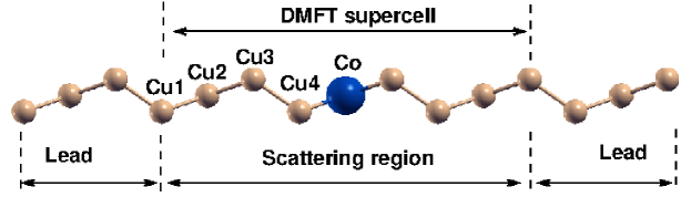
Figure 1: (color online) Schematic representation of the supercell used in calculations. The length of the cell and the distances between Cu1, Cu2, Cu3, Cu4 and Co are given in the text. The unit cell dimensions of the leads are kept at the relaxed bulk value 3.65 Å.

III Results

In this section we discuss the changes in the electronic structure and in the conductance of a single Co layer sandwiched between semi-infinite Cu electrodes caused by the inclusion of the Coulomb interaction at the GGA+DMFT level. The chosen values for Coulomb and exchange parameters for the $3d$-Co orbitals are $U=3$ eV and $J=0.9$ eV, while no interaction beyond GGA is considered for the $3d$-Cu states neither in the scattering region nor in the leads. The values of $U$ and $J$ are sometimes used as fitting parameters, although it is possible, in principle, to compute the dynamic electron-electron interaction matrix elements with good accuracy [60]. The static limit of the energy-dependent screened Coulomb interaction leads to a $U$ parameter in the energy range between 2 and 4 eV for all $3d$ transition metals, with substantial variations related to the choice of the local orbitals [61]. As the $J$ parameter is not affected by screening it can be calculated directly within LSDA; it turns out to be about the same for all $3d$ elements, $J$ $\approx$ 0.9 eV [49]. The sensitivity of results to $U$ and $J$ will be briefly addressed towards the end of this section. As regards the temperature, two values $T=80$ K and $200$ K are addressed. Smaller temperatures could be considered; however, this would strongly increase the computational efforts connected with the analytical continuation of the data onto the real axis.

III.1 Electronic structure calculations

The total density of states (DOS) for the Cu-Co-Cu heterostructure is shown in Fig. 2(a). The Co contribution to the total DOS, attributed to the atomic sphere radius of 2.69 $a_{0}$, is presented in Fig. 2(b). For comparison we plot in Fig. 2(c) the Co DOS in the bulk fcc structure, with the same atomic sphere radius.

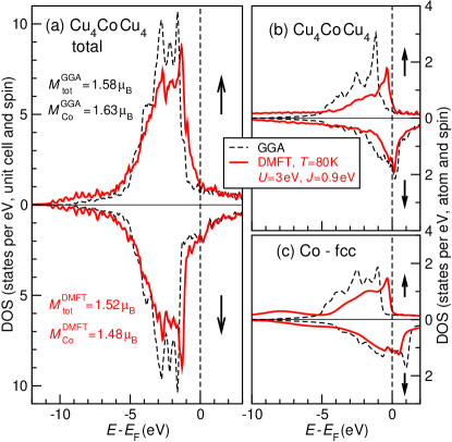
Figure 2: (Color online) Densities of states calculated by EMTO in relaxed geometries. Dashed black lines: GGA results; solid red lines: GGA+DMFT results. (a) Total DOS per scattered region; (b) local DOS per central Co atom of the heterostructure; (c) local DOS per atomic sphere of the same size in pure fcc bulk cobalt. The values of total and local Co magnetic moments for the scattered region are indicated in (a).

We start with discussing the features of the electronic structure of bulk Co. For the majority-spin electrons, the GGA DOS (Fig. 2c) is fully occupied. In the minority spin-channel, the Fermi level falls between two pronounced peaks at $\sim E_{F}\pm$1 eV. The orbital occupations are shown in Tab. 1. According to the GGA results the majority spin-up channel has a nominal $d$-occupation of $4.70$ while for minority electrons the occupation amounts to $2.87$. The $s$-electrons carry a negligible polarization, while $p$-electrons are slightly spin-polarized with a sign opposite to the main $d$-polarization which establishes a magnetic moment of $1.74~{}\mu_{B}$. As a consequence of the local Coulomb interactions parameterized by $U$ and $J$ within DMFT, the DOS distribution changes considerably. The overall broadening is strongly modified by the imaginary part of the self-energy. The top of the occupied $d$-band in the majority spin channel is shifted closer to the Fermi level, and some redistribution of the spectral weight occurs. These changes do not noticeably affect the occupation of $s$-orbitals, however, the magnetic moment, mostly due to $d$ electrons, is significantly reduced from $1.74~{}\mu_{\rm B}$ to $1.41~{}\mu_{\rm B}$.

Table 1: Orbital occupations and magnetic moments for the Cu-Co-Cu heterostructure and bulk Co-fcc. The DMFT calculations have been performed for $T$ = 200 K, $U$ = 3 eV, $J$ = 0.9 eV.

	$n^{\rm GGA}$			$M^{\rm GGA}$	$n^{\rm DMFT}$			$M^{\rm DMFT}$
Atom	$s(\downarrow\!/\!\uparrow)$	$p(\downarrow\!/\!\uparrow)$	$d(\downarrow\!/\!\uparrow)$	($\mu_{\rm B}$)	$s(\downarrow\!/\!\uparrow)$	$p(\downarrow\!/\!\uparrow)$	$d(\downarrow\!/\!\uparrow)$	($\mu_{\rm B}$)
Co bulk-fcc:
Co:	(0.34/0.33)	(0.39/0.31)	(2.87/4.70)	1.74	(0.34/0.33)	(0.38/0.35)	(3.04/4.50)	1.41
Cu4CoCu4 scattering region:
Cu1-3:	(0.36/0.36)	(0.33/0.33)	(4.78/4.78)	0.00	(0.39/0.39)	(0.45/0.45)	(4.72/4.72)	0.00
Cu4:	(0.36/0.36)	(0.36/0.33)	(4.76/4.79)	0.00	(0.38/0.37)	(0.42/0.39)	(4.58/4.65)	0.02
Co:	(0.33/0.32)	(0.33/0.31)	(2.96/4.63)	1.63	(0.32/0.33)	(0.33/0.37)	(2.70/4.13)	1.48

Essentially the correlation effects are determined not only by the magnitude of the local Coulomb parameters ($U,J$), but also by the orbital occupations. It was argued [62, 63] that electronic interactions may lead to the creation of either a majority-spin or a minority-spin hole. As the majority-spin channel is essentially full, there is effectively no space for excitations just across the Fermi level. On the contrary, in the minority-spin channel one finds a high density of electrons which can be immediately excited, leaving back holes. Such an occupation asymmetry has consequences concerning possible interaction channels in the multi-orbital Hubbard model: A majority-spin hole can only scatter with opposite-spin particles, which would cost an effective interaction $U$, while a minority-spin hole may also scatter with parallel-spin particles with the effective interaction $U-J<U$ [64]. Therefore correlation effects are expected to manifest themselves differently for majority- and minority-spin electrons.

Many DOS features of Co in the heterostructure geometry (Fig. 2b) resemble those of bulk cobalt (Fig. 2c), the occupation numbers of which are also given in Tab. 1. As expected, the spin polarization in $s$- and $p$-channels is very small; moreover it is opposite to the $d$-electrons, yielding an overall magnetic moment of $1.63~{}\mu_{B}$. As compared to the GGA case for the central Co layer of the heterostructure, in GGA+DMFT the Co $s$- and $p$-electron spin polarization changes sign, and the $d$-electrons spin splitting decreases. In the Cu-Co-Cu heterostructure geometry the Co-$d$ orbitals experience hybridization with the neighboring Cu-$d$ orbitals which leads to a change in the DOS of the Cu-layer in the vicinity of the Co-layer.

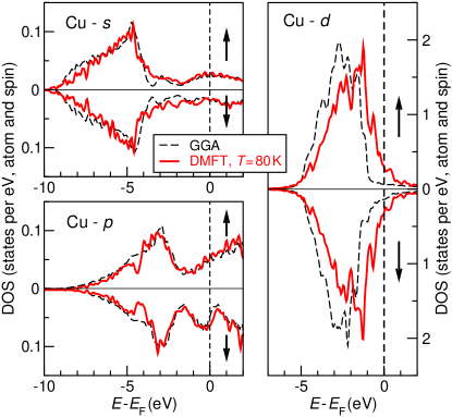
Figure 3: (Color online) Orbital resolved DOS for Cu4 in the Cu₄CoCu₄ heterostructure computed within the GGA (black-dashed line) and GGA+DMFT (red solid line) for $U=3$ eV and $J=0.9$ eV.

Figure 3 depicts the local DOS of the Cu atom closest to the Co monolayer (indicated Cu4 in Table 1). Even as no on-site interaction terms have been added to the $3d$-Cu states, the Co self-energy has a large impact on the GGA-DMFT density of states. In fact, the $3d$-Cu4 states are strongly coupled with the correlated $3d$-Co states and are dragged towards the Fermi energy, thus increasing the hybridization with the $4s$- and $4p$-Cu4 states. In contrast, the three outmost (from Co) copper layers Cu3, Cu2, Cu1 have very similar orbital occupations which slightly differ from those of the Cu4. The inclusion of interaction in the spirit of DMFT has only a slight effect upon the orbital occupations within Cu3, Cu2, and Cu1 as compared to Cu4 (see Table 1). Essentially the $4s$- and $4p$-Cu4 orbitals slightly increase in occupation, while $3d$-orbitals are depleted accordingly. At the same time, the minority/majority spin contrast gets enhanced: from $4.76/4.79$ in GGA to $4.58/4.65$ in GGA+DMFT. The spectral weight transfer in the Co layer – a consequence of electron correlations – modifies slightly, through $d-d$ hybridization, the spin asymmetry in $d$-holes of the closest copper layer inducing a magnetic moment.

We note that the temperature dependence of the DOS is negligible, and the effectiveness of electronic correlations is not significantly different in the heterostructure, as compared to the case of pure-Co fcc bulk.

Table 2: Effective mass enhancements $(m^{\ast}/m)^{\uparrow,\downarrow}$ for different bands of $d$-symmetry, calculated according to Eq. (5) as a function of the Coulomb and the exchange parameter, $U$ and $J$.

$U$ (eV)	$J$ (eV)	$xy_{\downarrow}$	$yz_{\downarrow}$	$z^{2}_{\downarrow}$	$xy_{\uparrow}$	$yz_{\uparrow}$	$z^{2}_{\uparrow}$
1	0.3	1.551	1.703	1.617	1.578	1.737	1.656
2	0.6	1.625	1.797	1.698	1.654	1.837	1.743
3	0.9	1.661	1.791	1.703	1.697	1.856	1.753

These changes are typical for correlation effects in transition metals, where the self-energy near the Fermi level has Fermi-liquid character: for the imaginary part, we have $-\mathrm{Im}\Sigma^{\sigma}_{MB,\alpha}(E)\propto E^{2}$, whereas the real part has negative slope, $\partial\mathrm{Re}\Sigma_{\mathrm{MB},\alpha}^{\sigma}(E)/\partial E<0$. Here $E$ is the energy relative to the Fermi level, and $\alpha$ numbers the three groups of $d$ states in hexagonal symmetry, $(z^{2})$, $(xz,yz)$ and $(x^{2}-y^{2},xy)$. From the self-energy we can also evaluate the mass enhancement [38], which within DMFT amounts to

$$\left(\frac{m^{*}}{m_{b}}\right)^{\sigma}_{\alpha}=1-\frac{\partial}{\partial E}{\rm Re}\ \Sigma_{\mathrm{MB}}^{\sigma,\alpha}(E),$$ (5)

where $m_{b}$ represents the band-mass obtained within the GGA calculations.

The values are given in Table 2, and we note that the enhancement factors for all orbitals are similar, in the range of $1.6-1.8$, which indicates that the system is medium-correlated.

III.2 Transport properties

Turning to transport properties, we display in Fig. 4(a) the total and spin-resolved transmission probabilities computed with GGA and GGA+DMFT. The spin-resolved transmission probability, $T_{\sigma}(E)$, is obtained from the k-dependent transmission, Eq. (2), by integrating over all $\mathbf{k}_{\parallel}$-points, so that $T_{\sigma}(E)=\frac{1}{\Omega_{\mathrm{BZ}}}\int_{\mathrm{BZ}}d\mathbf{k}_{\parallel}T_{\sigma}(\mathbf{k}_{\parallel},E)$. By inspecting Fig. 4(a) it can be seen that the overall transmission is a smooth function of energy, and has a rather large value of about 0.5 $e^{2}/h$ in both spin channels for most considered energies, which reflects the fact that we deal with an all-metal junction. In GGA the transport is mainly dominated by the Cu-$4s$, -$4p$ states, which are transmitted across the Co layer passing through the Co $4s$ states, while the Co $3d$ states do not contribute significantly to the transmission in this energy range. The Cu $3d$ states contribute to the transmission only at energies below $-1.5$ eV. Note that the GGA+DMFT transmission is always smaller than the GGA one. The black arrows in Fig. 4(a) indicate the energies at which a significant departure between the GGA+DMFT and the GGA transmission is observed. Specifically, the spin down transmission drops at about $0.3$ eV below the Fermi level, where the Co $3d$ DOS is high in the DMFT results, while the GGA transmission stays rather constant. In contrast, the spin-up transmission shows a “bump”, which extends over a region of about $2$ eV around the Fermi level. The slight dip within this bump at about $-$0.5 eV is at the same energy as the peak in the Co 3$d$ DOS, and represents a Fano-type reduction of transmission in such a metallic system due to interference of electrons in different conducting channels [31, 32, 65]. In our calculations this feature is a consequence of electronic correlations on the Co atom, which through the $d-d$ hybridization induce spin-polarization of the $3d$-Cu4 states and simultaneously produce the shift in the DOS of Fig. 3. In general, we note that for such all-metal systems the relation between DOS and transmission is non-trivial, since interference effects can lead to enhanced transmission also for energies with low DOS; alternatively, for high DOS the increased number of pathways for electrons can lead to a decrease of transmission.

From a many-body perspective, the added self-energy contributes in dephasing the electrons during the flow through the scattering region, so that the Landauer transmission computed with the many-body Green’s function is expected to be reduced in comparison with the DFT case. In principle, the opposite effect, namely the effective in-flow of electrons from the many-body self-energy “electrode” into the scattering region, would tend to increase the transmission. However, this in-flow process is not included in our calculations, as it is related to the vertex corrections [45].

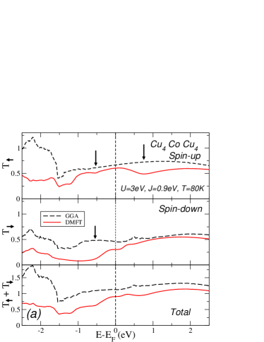
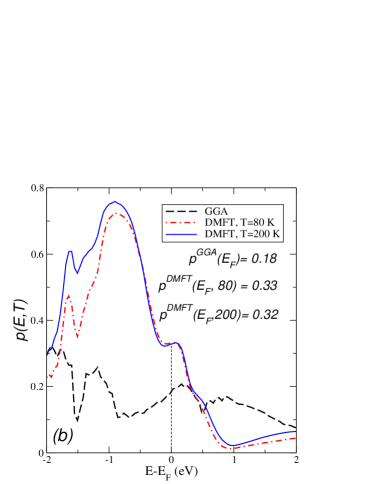
Figure 4: (Color online) Left: Spin-resolved transmission: majority-spins $T_{\uparrow}$ (upper panel), minority spins $T_{\downarrow}$ (middle panel) and total (lower panel). Black-dashed/red-solid lines are the GGA/GGA+DMFT results. Right: Transmission spin polarization around the Fermi energy GGA (black-dashed) and at finite temperatures T=80K (red-dotted-dashed), $T=200$ K(blue solid). The Coulomb and exchange parameters are $U=3$ eV, $J=0.9$ eV.

The spin polarization of the transmission is computed according to the formula

$$p(E_{\rm F})=\frac{T_{\uparrow}(E_{F})-T_{\downarrow}(E_{F})}{T_{\uparrow}(E_{F})+T_{\downarrow}(E_{F})},$$ (6)

for either DFT, or DFT+DMFT, where $T_{\sigma=\uparrow,\downarrow}$ is the transmission for the spin channel $\sigma$. The spin polarization in transmission obtained by GGA yields $p^{\rm GGA}(E_{F})=0.18$ [see also Fig. 4(b)], while the GGA+DMFT value reaches 0.33 at the Fermi level, and increases up to almost 0.8 at slightly lower energies. These results demostrate that electronic correlations may be decisive and lead to an increase in the spin polarization of transmission. As seen in Fig. 4(b), the enhancement in the spin polarization with respect to the GGA result is essentially temperature independent in the energy range of $E_{F}\pm 0.5$eV. Therefore we conclude that the enhanced spin contrast in transmission is a many-body effect rather than a temperature fluctuation effect.

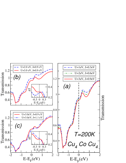
Figure 5: (Color online) Transmission for different values of Coulomb parameters: (a) with a fixed ratio $U/J$, (b) fixed $J$ and (c) fixed $U$, at $T=200$ K.

Finally, we test how the results for the transmission depend on the strength of the local Coulomb interaction parameters $U$ and $J$. The interaction matrix elements $U_{mm^{\prime}m^{\prime\prime}m^{\prime\prime\prime}}$ are usually parametrized using Slater integrals ($F^{k}$) with $k=0,2,4$ [49]. Accordingly the Hubbard $U$ parameter is constructed as a simple average over all possible pairs of correlated orbitals and is identified with the Slater integral $U=F^{0}$. The other Slater integrals $F^{2},F^{4}$ are fitted to the multiplet structure measured in X-ray photoemision [66]. An empiric relation has been introduced which connects the magnitude of the second and forth order Slater integrals, $F^{4}/F^{2}\approx 0.625$ [67]. The Hund’s exchange $J$ is expressed in terms of $F^{2}$ and $F^{4}$ which for the $d$-shell takes the form $J=(F^{2}+F^{4})/14$ [68], therefore the knowledge of the $(U,J)$-pair allows to compute all the matrix elements $U_{mm^{\prime}m^{\prime\prime}m^{\prime\prime\prime}}$. In Fig. 5(a) we plot the transmission (computed at $200$ K) keeping the ratio $U/J=1.0/0.3$ constant. While scaling the ratio $\alpha\cdot U/J$ with $\alpha=1,2,3$ we observe a monothonic reduction of the transmission at the Fermi level. This result is expected, as the matrix elements of the interaction are scalled in magnitude. In the same time, larger mass enhancement factors are obtained as $\alpha$ increases (see Tab. 1). Consequently we may conclude that the heavier the electron is, the smaller is the transmission at the Fermi level. Within $\pm 0.15$ eV of the Fermi level, a flat region in the transmission can be seen. Beyond these ranges, we note that below the Fermi level, down to $-$1 eV from it, the transmission decreases almost indiscriminately for different values of $(U,J)$. In the positive energy range up to roughly $+1$ eV, on the contrary, the transmission values differ, with larger $(U,J)$ resulting in lower transmission.

In Fig. 5(b) we display the dependence on parameters differently keeping $J=0.9,$ eV constant and varying $U$. We note that with higher $U$, the flat region centered at $E_{\rm F}$ shrinks a bit, which can be traced back to a stronger presence of $d$ orbitals in the correlated transmission. The inset of Fig. 5(b) depicts the “contrast” or spin difference in transmission: $\Delta T(E)=T_{\uparrow}(E)-T_{\downarrow}(E)$. The spin contrast changes slope as $U$ varies, from markedly positive $d(\Delta T)/dE$ at $E_{\rm F}$ for $U=2$ eV to roughly zero for $U=3$ eV.

In Fig. 5(c), on the contrary, the $U$ parameter is kept fixed to a “good” (yielding large flat region) value $U=3$ eV, and two different values are taken for the $J$ parameter. On increasing $J$, the flat region around $E_{\rm F}$ gets further reduced. Simultaneously (as seen in the inset and contrary to the behavior depicted in Fig. 5b), $\Delta T(E)$ acquires a negative slope. The change in the slope is potentially an interesting effect to be exploited in thermoelectric transport.

IV Conclusion

In this work we studied the effects of local electronic interactions and finite temperatures upon the transmission across the Cu₄CoCu₄ metallic heterostructure. Electronic structure calculations were performed using GGA and GGA+DMFT, assuming a local Coulomb interaction in the Co layer. We used a fully rotationally invariant Coulomb interaction on cobalt $d$-orbitals. The effective mass enhancement ratio for all orbitals is in the range of $1.6$ to $1.8$, suggesting that we deal with medium correlated system. Concerning the density of states, the presence of Coulomb interactions leads to a shift of the majority-spin channel of Co $d$-orbitals towards the Fermi level and to a redistribution of the spectral weights. In the minority spin-channel, the changes are less pronounced. This difference leads to different correlation effects for the majority- and minority-spin electrons. All these causes a decrease of the overall Co magnetic moment (with a predominant $d$ character) from $1.63~{}\mu_{B}$ (GGA)to $1.48~{}\mu_{B}$ (GGA+DMFT).

The transmission probability has been computed combining two different ab-initio codes, EMTO and Siesta/Smeagol. In order to transfer the many-body self-energy computed within the EMTO code into Siesta/Smeagol, we used a nearly unitary transformation which can be determined by requiring that the expectation value of the occupation matrix should be representation independent. The methodology was illustrated for a two-orbitals model (see Appendix B) and was carried out numerically for the Cu₄CoCu₄ heterostructure. Note that such a transformation is rather general and can be used in transfering quantities between two different implementations. Several tests confirmed that the proposed method is robust and numerically stable. With this combination of methods we have studied the transmission as a function of temperature and Coulomb parameters, which reveals the metallic character of the system considered. Substantial differences in the conducting processes, related to the presence of local Coulomb interaction in the cobalt layer were observed, due to changes in the electronic structure. Generally the transmission decreases with interaction, although the relation between changes in the electronic configuration and the transmission is highly non-trivial, due to interference effects. With electron correlations properly taken into account, the total transmission at the Fermi level drops by about $20\%$, whereas its spin polarization (spin contrast) increases by about $40\%$. These effects are entirely a consequence of the electronic correlation, since the transmission is practically temperature independent in the range of $E_{F}\pm 0.5$ eV. This suggest that the enhanced spin contrast in transmission is fully a many-body effect. In order to quantify the spin polarization effects in the transmission, we studied the transmission difference $\Delta T(E)$. This quantity clearly displays a strong dependence on the Coulomb parameters.

In conclusion, we have shown that electronic correlations may considerably affect the transmission and spin filter properties of heterostructures, even though the correlations would be classified only as “medium” when considering the effective mass enhancement. Hence results based on studies neglecting electronic correlations, which are numerous, must be interpreted with caution.

APPENDIX

Appendix A SIESTA and EMTO density of states

Inorder to demonstrate the reliability of both codes concerning the electronic structures, we present below the density of states for the heterostructure (Fig. 6). A rather good agreement is apparent.

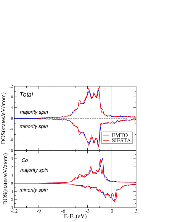
Figure 6: (color online) Total (unit cell) and Co density of states computed within the Siesta and EMTO technique.

Appendix B Matrix elements of the self-energy in the NAO basis set

The matrix representation of the self-energy operator is determined by the chosen basis. Within the EMTO basis set it has the form $\delta_{RR^{\prime}}{\tilde{\Sigma}}_{RL,RL^{\prime}}^{\sigma}(z)$. Here $R$ and $R^{\prime}$ are site indices while the $L$ symbol labels the orbital quantum numbers. To compute the transmission/conductance it is desirable to work within the Siesta/Smeagol basis. We emphasize that the major part of calculation is done within the Siesta+Smeagol package.

Since significant methodological differences exists between Siesta and EMTO, in the following we discuss the methodology of data transfer between the two codes. We describe briefly the most significant differences. The former (Siesta) implementation uses norm-conserving pseudopotentials, whereas the latter (EMTO) uses an all-electron formulation. Siesta uses no shape approximation with respect to the potential, whereas EMTO relies on the muffin-tin concept [34, 36]. Basis functions in Siesta are atom-centered numerical functions, whose angular parts are spherical harmonics, and radial parts are strictly confined numerical functions. A tradition finding its origins in quantum chemistry suggests that, in order to improve variational freedom of the basis set, more than one radial function is adopted into the basis for a given angular combination $(l,m)$, referred to as “multiple-$\zeta$” basis orbitals.

Even as Siesta maintains flexibility in constructing the basis set out of different “zetas”, possibly including moreover “polarization orbitals” and allowing a variety of schemes to enforce confinement, we shall stick in the following to the case of just “double-$\zeta$”, i.e., $2{\times}5=10$ basis functions, provided to accurately describe the $3d$ states on each cobalt atom. We shall fix some notation for further reference. The cumulate index of a basis function will be $\mu{\equiv}\{Ilm\zeta\}$, where $I$ indicates the atom carrying the basis function, $\zeta$ numbers the “zeta”s ($=1$ or $2$ in our case), and the $(l,m)$ is the conventional angular moment index. It should be noted, however, that Siesta employs real combinations of “standard” spherical harmonics, so that the indices $m={-2}$ through $2$ for $l=2$ correspond to $xy$, $yz$, $3z^{2}\!-\!r^{2}$, $xz$ and $x^{2}\!-\!y^{2}$ $d$-functions, correspondingly. With the above notation, the $i$th eigenstate of the Kohn–Sham Hamiltonian will expand into the basis functions $\phi_{\mu}$ as follows:

$$\Psi_{i}({\bf r})=\sum\limits_{\mu}c_{\mu i}\,\phi_{\mu}({\bf r}-{\bf R}_{I})\,,$$ (7)

and the variational principle yields the expansion coefficients [33]. Within the EMTO, the $d$-orbitals manifold is constructed using a basis set with real harmonics (physical orbitals representation), and the occupation matrix is obtained integrating the complex contour Green’s function (properly normalized path operator) in terms of the exact muffin-tin orbitals $\Psi_{RL}(\epsilon,{\bf r})$ corresponding to the energy $\epsilon$ [34, 35, 36]. On the other hand, in Siesta the numerical basis set is not restricted to the physical orbitals and allows the definition of simple/double $\zeta$ “atomic-like” representations. Enhancing the numerical atomic orbitals basis vectors does not affect the dimension of the vector spaces (in both cases the $d$-subspace), however, it complicates the algebra for the transformation matrix. The transformation involves the double zeta basis set, $\phi_{\mu}$, which for the $L(l,m)$-manifold contains $2(2l+1)$ components splitted into the first $(2l+1)-$single-zeta and the second $(2l+1)-$double-zeta components. First we write the explicit form for the EMTO orbital in a vector form for the $L(l=2,m=2l+1)$ subspace $|\Psi_{RL}(\epsilon,{\bf r})\rangle$, and the corresponding Siesta basis vector in the double $\zeta$-basis, $|\phi_{RL}({\bf r})\rangle=(\phi^{1\zeta}({\bf r}),\phi^{2\zeta}({\bf r}))$. The general transformation matrix $V_{m_{i},m_{j}}^{1\zeta,2\zeta}(\epsilon)$ is defined as the inner products of $\Psi_{R^{\prime}L^{\prime}}(\epsilon,{\bf r})$ with Siesta’s double-$\zeta$ basis, and takes the form of a dyadic product:

$$V_{m_{i},m_{j}}^{1\zeta,2\zeta}(\epsilon) = \langle\Psi_{R^{\prime}L^{\prime}}(\epsilon,{\bf r})|\otimes|\phi_{RL}({\bf r})\rangle=|\Psi_{RL}(\epsilon,{\bf r})\rangle^{T}|\phi_{RL}({\bf r})\rangle$$

$$= \begin{pmatrix}V_{m_{i},m_{j}}^{1\zeta}(\epsilon)\\ V_{m_{i},m_{j}}^{2\zeta}(\epsilon)\end{pmatrix}$$

The definition Eq. (B) for the $V$ matrix suggests the possibility of an explicit construction. However, a couple of obvious ambiguities may arise: (i) the transformation carries an energy dependence originating from the energy dependence of the EMTO orbitals [34, 35, 36], in contrast to the NAO basis set that is energy independent; (ii) normalization of the scattering path operator of EMTO is performed in a particular screened representation [34, 35, 36], a more involved procedure in comparison with the straight normalization of the NAO basis set.

Moreover, it is important to keep in mind that the closure relations that are typically used to build the matrix transformations are valid on the Hilbert space spanned by the eigenvectors of the Hamiltonian. These relations hold exactly for the numerical results of each code separately; nevertheless, the numerical results produced by different codes are not identical in the mathematical sense. Small differences between the observables computed with different codes may exist due to various factors – from unwanted numerical roundoff errors to incompleteness of the basis sets. This indicates that the closure relation for the Hilbert space of the EMTO will not be exact (in the mathematical since) when used in the Hilbert space spanned by the eigenvectors of Siesta. Consequently, we expect that the transformation matrix will fulfill the usual requirements (i.e., unitarity) only within numerical inaccuracies.

In view of these formal difficulties in obtaining a basis transformation to match a multiple scattering method with a Hamiltonian based scheme we propose an approach using the fact that expectation values should be independent of the specific representation. We apply this fundamental concept of quantum mechanics to the orbital occupation matrix (density matrix, $n_{m_{i},m_{j}}$) for the $d$-manifold (i.e., $m_{i},m_{j}=1,...,5$), and we look for a formally similar matrix transformation $W$:

$$\begin{pmatrix}W_{m_{j},m_{i}}^{1\zeta}&W_{m_{j},m_{i}}^{2\zeta}\end{pmatrix}n^{\rm EMTO}_{m_{i}m_{j}}\begin{pmatrix}W_{m_{i},m_{j}}^{1\zeta}\\ W_{m_{i},m_{j}}^{2\zeta}\end{pmatrix}=n^{\rm SIESTA}_{m_{i},m_{j}}$$ (9)

Equation (9) provides us with a system of equations to determine the matrix elements of $W$ numerically. Indeed, by inspecting the diagonal elements of the occupation matrix for the $xy$, $yz$, $z^{2}-r^{2}$, $xz$ and $x^{2}-y^{2}$ orbitals respectively, we obtained the data shown in Table 3. One should note that in the physical-EMTO basis the occupation matrix is diagonal. The corresponding Siesta occupation matrix has non-diagonal elements that are about two orders of magnitude smaller than the diagonal ones.

		$m_{i}=xy$	$yz$	$z^{2}-r^{2}$	$zx$	$x^{2}-y^{2}$
$n_{m_{i},m_{i}}^{EMTO}$	$\uparrow$	0.629	0.526	0.658	0.526	0.629
	$\downarrow$	0.922	0.925	0.908	0.925	0.922
$n_{m_{i},m_{i}}^{Siesta}$	$\uparrow$	0.639	0.485	0.784	0.485	0.639
	$\downarrow$	0.935	0.952	0.924	0.952	0.935

Table 3: Occupation matrix of Co-d orbitals in the Co/Cu heterostructure

While the symmetry and the qualitative trends in the occupations are the same, the exact numerical values are not. In other words, Eq. (9) is an approximative (numerical) relation, however, the resulting $W$ matrix reflects the symmetry of $n_{m_{i},m_{i}}$. The non-zero elements on the diagonal are close to $1$ for the first-$\zeta$ block and take small imaginary values for the second-$\zeta$ one. The equations Eq. (16) and (19) provide explicit values.

Accordingly, given the matrix elements for the transformation matrix, the self-energy generated in the EMTO-basis set can be transferred to the double(multiple)-zeta Siesta basis set according to

$$\Sigma^{\rm SIESTA}=W\Sigma^{\rm EMTO}W^{\dagger}.$$ (10)

In the following, we give simple examples to illustrate the self-energy transformation from the physical into a numerical double-zeta basis.

B.1 Example: a two orbital model in the cubic symmetry

We consider a simplified case of a diagonal self-energy corresponding to a two orbital model in the cubic symmetry. The self-energy and the “occupation” matrix can be written as:

$$\Sigma^{EMTO}(z)=\begin{pmatrix}\Sigma_{1}&0\\ 0&\Sigma_{2}\end{pmatrix};\ n^{EMTO}=\begin{pmatrix}{n}_{1}&0\\ 0&{n}_{2}\end{pmatrix}.$$ (11)

In such a case all inner products of the type $\langle\Psi_{m_{i}}(\epsilon,{\bf r})|\phi^{\zeta_{1}}_{m_{j}}(\bf r)\rangle$ are zero unless $m_{i}=m_{j}$, such that the transformation matrix has a generic form:

$$W_{m_{i},m_{i}}^{1\zeta,2\zeta}(\epsilon)=\begin{pmatrix}W^{1\zeta}_{11}&0\\ 0&W^{1\zeta}_{22}\\ W^{2\zeta}_{11}&0\\ 0&W^{2\zeta}_{22}\\ \end{pmatrix}.$$ (12)

Re-writing Eq. (9):

$$\begin{pmatrix}W^{1\zeta}_{11}&0\\ 0&W^{1\zeta}_{22}\\ W^{2\zeta}_{11}&0\\ 0&W^{2\zeta}_{22}\\ \end{pmatrix}\cdot\begin{pmatrix}{n}_{1}&0\\ 0&{n}_{2}\end{pmatrix}\cdot\begin{pmatrix}W^{1\zeta}_{11}&0&W^{2\zeta}_{11}&0\\ 0&W^{1\zeta}_{22}&0&W^{2\zeta}_{22}\end{pmatrix}=\begin{pmatrix}{\tilde{n}}_{1}^{1\zeta}&0&0&0\\ 0&{\tilde{n}}_{2}^{1\zeta}&0&0\\ 0&0&{\tilde{n}}_{1}^{2\zeta}&0\\ 0&0&0&{\tilde{n}}_{2}^{2\zeta}\\ \end{pmatrix}$$ (13)

one finds

$$W_{m_{i},m_{i}}^{1\zeta,2\zeta}(\epsilon)=\begin{pmatrix}\frac{\sqrt{{\tilde{n}}_{1}^{1\zeta}}}{\sqrt{n_{1}}}&0\\ 0&\frac{\sqrt{{\tilde{n}}_{2}^{1\zeta}}}{\sqrt{n_{2}}}\\ \frac{\sqrt{{\tilde{n}}_{1}^{2\zeta}}}{\sqrt{n_{1}}}&0\\ 0&\frac{\sqrt{{\tilde{n}}_{2}^{2\zeta}}}{\sqrt{n_{2}}}\\ \end{pmatrix},\$$ (14)

and accordingly the self-energy in the NAO basis-set has the form:

$$\Sigma=\begin{pmatrix}\Sigma_{1}\frac{{{\tilde{n}}_{1}^{1\zeta}}}{{n_{1}}}&0&\Sigma_{1}\frac{\sqrt{{\tilde{n}}_{1}^{1\zeta}{\tilde{n}}_{1}^{2\zeta}}}{n_{1}}&0\\ 0&\Sigma_{2}\frac{{\tilde{n}}_{2}^{1\zeta}}{n_{2}}&0&\Sigma_{2}\frac{\sqrt{{\tilde{n}}_{2}^{1\zeta}{\tilde{n}}_{2}^{2\zeta}}}{n_{2}}\\ \Sigma_{1}\frac{\sqrt{{\tilde{n}}_{1}^{1\zeta}{\tilde{n}}_{1}^{2\zeta}}}{n_{1}}&0&\Sigma_{1}\frac{{{\tilde{n}}_{1}^{2\zeta}}}{{n_{1}}}&0\\ 0&\Sigma_{2}\frac{\sqrt{{\tilde{n}}_{2}^{1\zeta}{\tilde{n}}_{2}^{2\zeta}}}{n_{2}}&0&\Sigma_{2}\frac{{\tilde{n}}_{2}^{2\zeta}}{n_{2}}\end{pmatrix}=\begin{pmatrix}\framebox{$\Sigma^{1\zeta,1\zeta}$}&\framebox{$\Sigma^{1\zeta,2\zeta}$}\\ \framebox{$\Sigma^{2\zeta,1\zeta}$}&\framebox{$\Sigma^{2\zeta,2\zeta}$}\end{pmatrix}$$ (15)

in which every $\Sigma^{i\zeta,j\zeta}$ is a $2\times 2$ block-diagonal matrix. There are a couple of conclusions to be drawn from the above simplified example: (i) as a consequence of the reduced weight in the second $\zeta$ occupation (at least 10 times smaller that in the single $\zeta$), the magnitude of the matrix elements of the self-energy in the NAO basis set follow the relation $\Sigma^{1\zeta,1\zeta}>\Sigma^{1\zeta,2\zeta}>\Sigma^{2\zeta,2\zeta}$; (ii) the existence of only-diagonal orbital occupations does not imply the existence of an unitary transformation, except for the case of numerical identical values for the occupation matrices in both basis. These observations do not change when the symmetry is lower than cubic and non-zero matrix elements on the non-diagonal of the occupation matrix appear.

Appendix C Transformation matrix for the Co-d manifold in the Cu-Co-Cu heterostructure

This section provides the spin-resolved matrix elements, $W_{\sigma=\uparrow,\downarrow}$, used in the calculation.

$$W_{\uparrow}=\left(\begin{array}[]{ccccc}1.024&0&0&0&0\\ 0&0.987&0&0&0\\ 0&0&1.096&0&0\\ 0&0&0&0.985&0\\ 0&0&0&0&1.024\\ 0.178i&0&0&0&0\\ 0&0.218i&0&0&0\\ 0&0&0&0&0\\ 0&0&0&0.218i&0\\ 0&0&0&0&0.178i\\ \end{array}\right).$$ (16)

The orthogonality can be checked using the following relations:

$$W_{\uparrow}^{\dagger}W_{\uparrow}=\left(\begin{array}[]{ccccc}1.016&0&0&0&0\\ 0&0.922&0&0&0\\ 0&0&1.202&0&0\\ 0&0&0&0.922&0\\ 0&0&0&0&1.016\\ \end{array}\right)$$ (17)

and

$$W_{\uparrow}W_{\uparrow}^{{}^{\dagger}}=\left(\begin{array}[]{cccccccccc}1.048&0&0&0&0&0.182i&0&0&0&0\\ 0&0.970&0&0&0&0&0.215i&0&0&0\\ 0&0&1.202&0&0&0&0&0&0&0\\ 0&0&0&0.970&0&0&0&0&0.215i&0\\ 0&0&0&0&1.047&0&0&0&0&0.182i\\ 0.182i&0&0&0&0&-0.032&0&0&0&0\\ 0&0.215i&0&0&0&0&-0.048&0&0&0\\ 0&0&0&0&0&0&0&0&0&0\\ 0&0&0&0.215i&0&0&0&0&-0.048&0\\ 0&0&0&0&0.183i&0&0&0&0&-0.032\\ \end{array}\right)$$ (18)

The corresponding transformation matrix for spin-down component reads:

$$W_{\downarrow}=\left(\begin{array}[]{ccccc}0.960&0&0&-0.007&0\\ 0&0.9572&0&0&-0.007\\ 0&0&0.967&0&0\\ -0.007&0&0&0.957&0\\ 0&-0.007&0&0&0.960\\ 0.304&0&0&-0.002&0\\ 0&0.337&0&0&-0.002\\ 0&0&0.287&0&0\\ -0.002&0&0&0.337&0\\ 0&-0.002&0&0&0.304\\ \end{array}\right)$$ (19)

$$W_{\downarrow}^{\dagger}W_{\downarrow}=\left(\begin{array}[]{ccccc}1.014&0&0&-0.015&0\\ 0&1.029&0&0&-0.015\\ 0&0&1.017&0&0\\ -0.015&0&0&1.029&0\\ 0&-0.015&0&0&1.014\\ \end{array}\right)$$ (20)

$$W_{\downarrow}W_{\downarrow}^{\dagger}=\left(\begin{array}[]{cccccccccc}0.922&0&0&-0.014&0&0.292&0&0&0&0\\ 0&0.916&0&0&-0.014&0&0.322&0&0&0\\ 0&0&0.935&0&0&0&0&0.278&0&0\\ -0.014&0&0&0.916&0&0&0&0&0.322&0\\ 0&-0.014&0&0&0.922&0&0&0&0&0.292\\ 0.297&0&0&0&0&0.092&0&0&0&0\\ 0&0.325&0&0&0&0&0.114&0&0&0\\ 0&0&0.278&0&0&0&0&0.083&0&0\\ 0&0&0&0.325&0&0&0&0&0.114&0\\ 0&0&0&0&0.292&0&0&0&0&0.092\\ \end{array}\right)$$ (21)

Appendix D Assessment of accuracy

In order to test the effect of the numerical inaccuracies occurring in the transformation matrix on the final results, we compute the total transmission by using a simplified model for the transformation matrix:

$$W^{1\zeta,2\zeta}_{Model}=\begin{pmatrix}\framebox{$W^{1\zeta}$}\\ \framebox{$W^{2\zeta}$}\end{pmatrix},$$ (22)

where $W^{1\zeta}=\alpha I$ and $W^{2\zeta}=\beta I$, where $I$ is the unity matrix. The results for $\alpha=0.9$, $\beta=0.1$; $\alpha=0.5$, $\beta=0.5$; and $\alpha=0.1$, $\beta=0.9$, respectively are given in Fig. 7. It can be clearly seen that even for such a crude approximation, the results for the first model (i.e., with a significant weight of the self-energy on the first zeta orbital) differ with only a few percent over large energy domains. For the occupied states, large values for $\Sigma^{1\zeta}$ provide already a good approximation for the transformation.

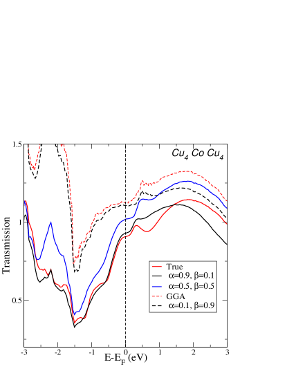
Figure 7: (color online) Comparison between the transmission functions obtained for different model-forms of $W^{1\zeta,2\zeta}$.

References

- Schep et al. [1995] K. M. Schep, P. J. Kelly, and G. E. W. Bauer, Phys. Rev. Lett. 74, 586 (1995).
- Schep et al. [1998] K. M. Schep, P. J. Kelly, and G. E. W. Bauer, Phys. Rev. B 57, 8907 (1998).
- de Groot et al. [1983] R. A. de Groot, F. M. Mueller, P. G. van Engen, and K. H. J. Buschow, Phys. Rev. Lett. 50, 2024 (1983).
- Zutic et al. [2004] I. Zutic, J. Fabian, and S. D. Sarma, Rev. Mod. Phys. 76, 323 (2004).
- Katsnelson et al. [2008] M. I. Katsnelson, V. Y. Irkhin, L. Chioncel, A. I. Lichtenstein, and R. A. de Groot, Rev. Mod. Phys. 80, 315 (2008).
- Landauer [1957] R. Landauer, IBM J. Res. Develop. 1, 223 (1957).
- Landauer [1988] R. Landauer, IBM J. Res. Develop. 32, 306 (1988).
- Bütikker [1986] M. Bütikker, Phys. Rev. Lett. 57, 1761 (1986).
- Bütikker [1988] M. Bütikker, IBM J. Res. Develop. 32, 317 (1988).
- Sanvito et al. [1999] S. Sanvito, C. J. Lambert, J. H. Jefferson, and A. M. Bratkovsky, Phys. Rev. B 59, 11936 (1999).
- Mathon et al. [1997] J. Mathon, A. Umerski, and M. Villeret, Phys. Rev. B 55, 14378 (1997).
- Tsymbal and Pettifor [2001] E. Y. Tsymbal and D. G. Pettifor, Phys. Rev. B 64, 212401 (2001).
- Krstić et al. [2002] P. S. Krstić, X.-G. Zhang, and W. H. Butler, Phys. Rev. B 66, 205319 (2002).
- Hohenberg and Kohn [1964] P. Hohenberg and W. Kohn, Phys. Rev. 136, B864 (1964).
- Kohn and Sham [1965] W. Kohn and L. J. Sham, Phys. Rev. 140, A1133 (1965).
- Kohn [1999] W. Kohn, Rev. Mod. Phys. 71, 1253 (1999).
- Wortmann et al. [2002a] D. Wortmann, H. Ishida, and S. Blügel, Phys. Rev. B 65, 165103 (2002a).
- Wortmann et al. [2002b] D. Wortmann, H. Ishida, and S. Blügel, Phys. Rev. B 66, 075113 (2002b).
- Stiles and Hamann [1988] M. D. Stiles and D. R. Hamann, Phys. Rev. B 38, 2021 (1988).
- MacLaren et al. [1999] J. M. MacLaren, X.-G. Zhang, W. H. Butler, and X. Wang, Phys. Rev. B 59, 5470 (1999).
- Rocha et al. [2006] A. R. Rocha, V. M. Garcí a Suárez, S. Bailey, C. Lambert, J. Ferrer, and S. Sanvito, Phys. Rev. B 73, 085414 (2006).
- Metzner and Vollhardt [1989] W. Metzner and D. Vollhardt, Phys. Rev. Lett. 62, 324 (1989).
- Georges et al. [1996] A. Georges, G. Kotliar, W. Krauth, and M. J. Rozenberg, Rev. Mod. Phys. 68, 13 (1996).
- Kotliar and Vollhardt [2004] G. Kotliar and D. Vollhardt, Physics Today 57, 53 (2004).
- Anisimov et al. [1997] V. I. Anisimov, A. I. Poteryaev, M. A. Korotin, A. O. Anokhin, and G. Kotliar, J. Phys.: Condens. Matter 9, 7359 (1997).
- Lichtenstein and Katsnelson [1998] A. I. Lichtenstein and M. I. Katsnelson, Phys. Rev. B 57, 6884 (1998).
- Koch et al. [2008] E. Koch, G. Sangiovanni, and O. Gunnarsson, Phys. Rev. B 78, 115102 (2008).
- Rocha et al. [2005] A. R. Rocha, V. M. Garcí a Suárez, S. Bailey, C. Lambert, J. Ferrer, and S. Sanvito, Nature Materials 4, 335 (2005).
- Rungger and Sanvito [2008] I. Rungger and S. Sanvito, Phys. Rev. B 78, 035407 (2008).
- Aoki et al. [2014] H. Aoki, N. Tsuji, M. Eckstein, M. Kollar, T. Oka, and P. Werner, Rev. Mod. Phys. 86, 779 (2014).
- Jacob et al. [2009] D. Jacob, K. Haule, and G. Kotliar, Phys. Rev. Lett. 103, 016803 (2009).
- Jacob and Kotliar [2010] D. Jacob and G. Kotliar, Phys. Rev. B 82, 085423 (2010).
- Soler et al. [2002] J. M. Soler, E. Artacho, J. D. Gale, A. García, J. Junquera, and P. Ordejón, J. Phys: Condens. Matter 14, 2745 (2002).
- Andersen and Saha-Dasgupta [2000] O. K. Andersen and T. Saha-Dasgupta, Phys. Rev. B 62, R16219 (2000).
- Vitos et al. [2000] L. Vitos, H. L. Skriver, B. Johansson, and J. Kollár, Comp. Mat. Sci. 18, 24 (2000).
- Vitos [2001] L. Vitos, Phys. Rev. B 64, 014107 (2001).
- Weinberger [1990] P. Weinberger, Electron Scattering Theory for Ordered and Disordered Matter (Clarendon Press, Oxford, 1990).
- Mahan [1990] G. D. Mahan, Many-Particle Physics (Plenum Press, New York, 1990).
- Datta [1995] S. Datta, Electronic Transport in Mesoscopic Systems, vol. 3 of Cambridge Studies in Semiconductor Physics and Microelectronic Engineering (Cambridge University Press, New York, 1995).
- Fisher and Lee [1981] D. S. Fisher and P. A. Lee, Phys. Rev. B 23, 6851 (1981).
- Taylor et al. [2001] J. Taylor, H. Guo, and J. Wang, Phys. Rev. B 63, 245407 (2001).
- Butler et al. [2001] W. H. Butler, X.-G. Zhang, T. C. Schulthess, and J. M. MacLaren, Phys. Rev. B 63, 054416 (2001).
- Rungger et al. [2009] I. Rungger, O. Mryasov, and S. Sanvito, Phys. Rev. B 79, 094414 (2009).
- Caffrey et al. [2012] N. M. Caffrey, T. Archer, I. Rungger, and S. Sanvito, Phys. Rev. Lett. 109, 226803 (2012).
- Oguri [2001] A. Oguri, J. Phys. Soc. Jpn. 70, 2666 (2001).
- Meir and Wingreen [1992] Y. Meir and N. S. Wingreen, Phys. Rev. Lett. 68, 2512 (1992).
- Chioncel et al. [2003] L. Chioncel, L. Vitos, I. A. Abrikosov, J. Kollar, M. I. Katsnelson, and A. I. Lichtenstein, Phys. Rev. B 67, 235106 (2003).
- Perdew et al. [1996] J. P. Perdew, K. Burke, and M. Ernzerhof, Phys. Rev. Lett. 77, 3865 (1996).
- Imada et al. [1998] M. Imada, A. Fujimori, and Y. Tokura, Rev. Mod. Phys. 70, 1039 (1998).
- Katsnelson and Lichtenstein [2002] M. I. Katsnelson and A. I. Lichtenstein, Eur. Phys. J. B 30, 9 (2002).
- Bickers and Scalapino [1989] N. E. Bickers and D. J. Scalapino, Ann. Phys. (N. Y.) 193, 206 (1989).
- Minár et al. [2005] J. Minár, L. Chioncel, A. Perlov, H. Ebert, M. I. Katsnelson, and A. I. Lichtenstein, Phys. Rev. B 72, 045125 (2005).
- Drchal et al. [2005] V. Drchal, V. Jani , J. Kudrnovsk , V. S. Oudovenko, X. Dai, K. Haule, and G. Kotliar, J. Phys.: Condens. Matter 17, 61 (2005).
- Kotliar et al. [2006] G. Kotliar, S. Y. Savrasov, K. Haule, V. S. Oudovenko, O. Parcollet, and C. A. Marianetti, Rev. Mod. Phys. 78, 865 (2006).
- Galitski [1958] V. M. Galitski, Zh. Eksper. Teor. Fiz. 34, 1011 (1958).
- Katsnelson and Lichtenstein [1999] M. I. Katsnelson and A. I. Lichtenstein, J. Phys.: Condens. Matter 11, 1037 (1999).
- Vidberg and Serene [1977] H. J. Vidberg and J. W. Serene, J. Low Temp. Phys. 29, 179 (1977).
- Lichtenstein et al. [2001] A. I. Lichtenstein, M. I. Katsnelson, and G. Kotliar, Phys. Rev. Lett. 87, 067205 (2001).
- Petukhov et al. [2003] A. G. Petukhov, I. I. Mazin, L. Chioncel, and A. I. Lichtenstein, Phys. Rev. B 67, 153106 (2003).
- Aryasetiawan et al. [2004] F. Aryasetiawan, M. Imada, A. Georges, G. Kotliar, S. Biermann, and A. I. Lichtenstein, Phys. Rev. B 70, 195104 (2004).
- Miyake and Aryasetiawan [2008] T. Miyake and F. Aryasetiawan, Phys. Rev. B 77, 085122 (2008).
- Monastra et al. [2002] S. Monastra, F. Manghi, C. A. Rozzi, C. Arcangeli, E. Wetli, H.-J. Neff, T. Greber, and J. Osterwalder, Phys. Rev. Lett. 88, 236402 (2002).
- Grechnev et al. [2007] A. Grechnev, I. Di Marco, M. I. Katsnelson, A. I. Lichtenstein, J. Wills, and O. Eriksson, Phys. Rev. B 76, 035107 (2007).
- Manghi et al. [1999] F. Manghi, V. Bellini, J. Osterwalder, T. J. Kreutz, P. Aebi, and C. Arcangeli, Phys. Rev. B 59, R10409 (1999).
- Calvo et al. [2009] M. R. Calvo, J. Fernandez-Rossier, J. J. Palacios, D. J. D. Natelson, and C. Untiedt, Nature 358, 1150 (2009).
- Anisimov and Gunnarsson [1991] V. I. Anisimov and O. Gunnarsson, Phys. Rev. B 43, 7570 (1991).
- de Groot et al. [1990] F. M. F. de Groot, J. C. Fuggle, B. T. Thole, and G. A. Sawatzky, Phys. Rev. B 42, 5459 (1990).
- Anisimov et al. [1993] V. I. Anisimov, I. V. Solovyev, M. A. Korotin, M. T. Czyżyk, and G. A. Sawatzky, Phys. Rev. B 48, 16929 (1993).