Bright solitons in a 2D spin-orbit-coupled dipolar Bose-Einstein condensate

Abstract

We study a two-dimensional spin-orbit-coupled dipolar Bose-Einstein condensate with repulsive contact interactions by both the variational method and the imaginary time evolution of the Gross-Pitaevskii equation. The dipoles are completely polarized along one direction in the 2D plane so as to provide an effective attractive dipole-dipole interaction. We find two types of solitons as the ground states arising from such attractive interactions: a plane wave soliton with a spatially varying phase and a stripe soliton with a spatially oscillating density for each component. Both types of solitons possess smaller size and higher anisotropy than the soliton without spin-orbit coupling. Finally, we discuss the properties of moving solitons, which are nontrivial because of the violation of Galilean invariance.

I introduction

Ever since the first achievement of Bose-Einstein condensates (BECs) in ultracold atomic gases BookSmith , matter wave solitons have been the central focus of many experimentalists and theorists KevrekidisBook . Solitons are the result of the interplay between nonlinearity and dispersion and keep their shape while traveling. In BECs, nonlinearity originates from collisional interactions between atoms, which can be readily tuned via Feshbach resonances Chin2010RMP . In general, there are two types of solitons: a bright soliton with a density bump for attractive interactions and a dark soliton with a density notch and a phase jump for repulsive interactions. Both bright and dark solitons have been experimentally observed in cold atoms with contact interactions Burger1999PRL ; Phillips2000Science ; Cornell2001PRL ; Hulet2002Nature ; Salomon2002Science ; Wieman2006PRL ; Oberthaler2004PRL ; Peter2013PRL ; Hulet2014Nature . However, for such contact attractive interactions, bright solitons can only exist in one dimension (1D), but not in two dimensions (2D) where the states either collapse or expand note0 .

Different from the local nonlinearity resulting from contact interactions, the non-local nonlinearity can stabilize a 2D bright soliton Wyller2001PRE ; Pfau2009RPP , in particular, the nonlinearity introduced by the dipole-dipole interaction. This interaction is long ranged and anisotropic with the strength and sign (i.e. repulsive or attractive) depending on the dipole orientation. When an external rotating magnetic field is applied to reverse the sign of the interaction Santos2005PRL , or the dipoles are completely polarized in a 2D plane Malomed2008PRL , the dipolar interaction can become attractive and 2D bright solitons can be, therefore, stabilized under appropriate conditions. It is essential to note that although the relevant interaction in common experiments with cold atomic gases is contact, increasing interest has been focused on the atoms with large magnetic moments that possess dipole-dipole interactions Pfau2009RPP ; Bohn2011PRL ; Zoller2012 . In fact, the Bose-Einstein condensation of several dipolar atoms such as Chromium Pfau2005PRL ; Pfau2008NatPhys ; Beaufils2008PRA , Dysprosium Lev2011PRL , and Erbium Ferlaino2012PRL , as well as the degeneracy of a dipolar Fermi gas Lev2012PRL ; Ferlaino2014PRL have been observed in experiments.

Recently, the spin-orbit coupling between two hyperfine states of cold atoms has been experimentally engineered  Lin2011Nature ; Jing2012PRL ; Zwierlen2012PRL ; PanJian2012PRL ; Peter2013 ; Spilman2013PRL . And this achievement has ignited tremendous interest in this field because of the dramatic change in the single particle dispersion (induced by spin-orbit coupling) which in conjunction with the interaction leads to many exotic superfluids Galitski2008PRA ; ZhaiHui2010PRL ; Wu2011CPL ; Ho2011PRL ; Santos2011PRL ; Yongping2012PRL ; Hu2012PRL ; Li2012PRL ; Chen2012PRA ; Kuei2015arXiv ; Yong2015arXiv (also see Ohberg2011RMP ; Spilman2013NatRev ; Xiangfa2013JPB ; Goldman2014RPP ; Zhai2015RPP ; WeiArxiv ; Jing2014 ; Yong2015JP for review). Such change in dispersion also results in exotic solitons even when the interaction is contact, including bright solitons Santos2010PRL ; Yong2013PRA ; Achilleos2014PRL ; Salasnich ; Malomed2014PRE ; Malomed2014PRA ; Sakaguchi , dark solitons Fialko ; Achilleos2013EL , and gap solitons Kartashov2013PRL ; Kartashov2014PRL ; Yongping2015arXiv for BECs, as well as dark solitons for Fermi superfluids Yong2014Soliton ; XJ2015PRA . These solitons exhibit unique features that are absent without spin-orbit coupling, for instance, the plane wave profile with a spatially varying phase and the stripe profile with a spatially oscillating density for BECs, as well as the presence of Majorana fermions inside a soliton for Fermi superfluids. Also, the violation of Galilean invariance Qizhong2013 ; Yong2013PRA ; QizhongReview by spin-orbit coupling dictates that the structure of solitons changes with their velocities.

On the other hand, spin-orbit-coupled BECs with dipole-dipole interactions Yi2012PRL ; Cui2013PRA ; Ng2014PRA ; Yousefi2014arXiv have also been explored, and intriguing quasicrystals Demler2013PRL as well as meron states Clark2013PRL have been found. However, whether a soliton can exist in such BECs in 2D with long ranged dipole-dipole interactions and spin-orbit dispersion has not yet been investigated.

In this paper, we examine the existence and properties of a bright soliton in a two species spin-orbit-coupled dipolar BEC in 2D with repulsive contact interactions via both the variational method and the imaginary time evolution of the Gross-Pitaevskii equation (GPE). The dipoles are completely oriented along the $y$ direction in the 2D plane in order to provide an effective attractive dipole-dipole interaction. Thanks to such attractive interactions, we find two types of solitons: a plane wave soliton (when the repulsive intraspecies contact interaction is larger than the repulsive interspecies one) and a stripe soliton (when the interspecies one is larger). These 2D solitons as the ground states cannot exist for a system with pure attractive contact interactions and spin-orbit coupling. Such solitons are highly anisotropic and their size is also reduced by spin-orbit coupling. Finally, we study the moving solitons, which are nontrivial because of the lack of Galilean invariance. The size of a soliton first increases and then decreases with the rise of the velocity and this change is anisotropic. The moving soliton also tends to be plane wave even when its stationary counterpart has the stripe structure.

The paper is organized as follows. In Sec. II, we introduce the energy functional and the time-dependent GPE, which are used to describe a spin-orbit-coupled dipolar BEC. In Sec. III, we calculate the bright soliton by performing the minimization of the energy of the variational ansatz wave functions and an imaginary time evolution of the GPE. The properties of such soliton are also explored by the former method. Then, we study the nontrivial moving solitons in Sec. IV. Finally, we conclude in Sec. V.

II Model

We consider a Rashba-type spin-orbit-coupled BEC and write its single particle Hamiltonian as

$$H_{s}=\frac{\hat{\bf p}^{2}}{2m}+\frac{1}{2}m\omega_{\perp}^{2}\rho^{2}+\frac{1}{2}m\omega_{z}^{2}z^{2}+\lambda(\hat{{\bf p}}\times{\bm{\sigma}})\cdot{\bf e}_{z},$$ (1)

where $\hat{\bf p}=-i\hbar\nabla$ is the momentum operator, $m$ is the atom mass, $\lambda$ is the spin-orbit coupling strength, and $\bm{\sigma}$ are Pauli matrices. $\omega_{\perp}$ ($\omega_{z}$) is the trap frequency in the $(x,y)$ plane (along the $z$ direction). Here, we assume that $\hbar\omega_{z}$ is much larger than $\hbar\omega_{\perp}$ and the mean-field interaction so that the atoms are frozen to the ground state in the $z$ direction. Given that a soliton is studied, we thus set $\omega_{\perp}=0$.

When the $s$-wave contact and dipole-dipole interactions are involved, the energy functional of a 2D condensate can be written as

$$E= \int d{\bf r}\left[\Psi({\bf r})^{\dagger}H_{s}\Psi({\bf r})+\frac{1}{2}g(|\Psi_{\uparrow}|^{4}+|\Psi_{\downarrow}|^{4})\right.$$ (2)

$$\left.+g_{12}|\Psi_{\uparrow}|^{2}|\Psi_{\downarrow}|^{2}\right]+E_{dd},$$

where the condensate wave function $\Psi({\bf r})=[\Psi_{\uparrow}({\bf r}),\Psi_{\downarrow}({\bf r})]^{T}$ with two pseudo-spin components $\Psi_{\uparrow(\downarrow)}({\bf r})$ , $g=4\pi\hbar^{2}a/(\sqrt{2\pi}l_{z}m)$ and $g_{12}=4\pi\hbar^{2}a_{12}/(\sqrt{2\pi}l_{z}m)$ are the intraspecies and interspecies contact interaction strength respectively with the intraspecies and interspecies $s$-wave scattering length being $a$ and $a_{12}$ and the characteristic length along $z$ being $l_{z}=\sqrt{\hbar/(m\omega_{z})}$. Here, $H_{s}=-\hbar^{2}(\partial_{x}^{2}+\partial_{y}^{2})/(2m)-i\hbar\lambda(\partial_{x}\sigma_{y}-\partial_{y}\sigma_{x})$ is the 2D single particle Hamiltonian, and the third dimension has been integrated out. For dipole-dipole interactions, we only consider the density-density interaction which is dominant when a two subspace (i.e. two pseudo-spin states) of a large spin atom (e.g. dysprosium) is considered. We also assume that the dipoles are all oriented along the $y$ direction, thus

$$E_{dd}=\frac{g_{d}}{2}\frac{1}{(2\pi)^{2}}\int d{\bf k}\rho_{\bf k}\rho_{-{\bf k}}U_{d}({\bf k}l_{z}),$$ (3)

where the Fourier transform of the total density is $\rho_{\bf k}=\int d{\bf r}e^{-i{\bf k}\cdot{\bf r}}(|\Psi_{\uparrow}|^{2}+|\Psi_{\downarrow}|^{2})$ and $U({\bf k})$ is given by

$$U_{d}({\bf k}l_{z})=-\sqrt{2\pi}+\frac{3\pi l_{z}k^{2}_{y}e^{k^{2}l_{z}^{2}/2}\text{erfc}(kl_{z}/\sqrt{2})}{k},$$ (4)

with erfc being the complementary error function. Here, $g_{d}=\mu_{0}\mu^{2}/(6\pi l_{z})$ characterizes the strength of the dipole-dipole interaction where $\mu$ is the magnetic dipolar moment and $\mu_{0}$ is the permeability of the free space.

The dynamical behavior of a BEC can be described by the time-dependent GPE

$$i\hbar\frac{\partial\Psi({\bf r})}{\partial t}=H_{s}\Psi({\bf r})+gG\Psi({\bf r})+g_{d}U_{d}({\bf r})\Psi({\bf r}),$$ (5)

where the contact interaction matrix is

$$G=\left(\begin{array}[]{cc}|\Psi_{\uparrow}|^{2}+\frac{g_{12}}{g}|\Psi_{\downarrow}|^{2}&0\\ 0&|\Psi_{\downarrow}|^{2}+\frac{g_{12}}{g}|\Psi_{\uparrow}|^{2}\\ \end{array}\right),$$ (8)

and the dipolar interaction potential is

$$U_{d}({\bf r})=\frac{1}{(2\pi)^{2}}\int d{\bf k}e^{i{\bf k}\cdot{\bf r}}\rho({\bf k})U_{d}({\bf k}l_{z}).$$ (9)

For numerical simulation, we choose $\hbar\omega_{z}$, $l_{z}$, and $1/\omega_{z}$ as the units of energy, length, and time, respectively, and the dimensionless energy per atom hence reads

$$\mathcal{E}= \int d{\bf r}\left[\Phi({\bf r})^{\dagger}\mathcal{H}_{s}\Phi({\bf r})+\frac{1}{2}\gamma(|\Phi_{\uparrow}|^{4}+|\Phi_{\downarrow}|^{4})\right.$$ (10)

$$\left.+\gamma_{12}|\Phi_{\uparrow}|^{2}|\Psi_{\downarrow}|^{2}\right]+\frac{\gamma_{d}}{2(2\pi)^{2}}\int d{\bf k}n_{\bf k}n_{-{\bf k}}U_{d}({\bf k}),$$

where $\mathcal{H}_{s}=-(\partial_{x}^{2}+\partial_{y}^{2})/2-i\alpha(\partial_{x}\sigma_{y}-\partial_{y}\sigma_{x})$, $\alpha=\lambda/(\omega_{x}l_{z})$, $\gamma=2\sqrt{2\pi}N_{0}a/l_{z}$, $\gamma_{12}=2\sqrt{2\pi}N_{0}a_{12}/l_{z}$ with the total particle number $N_{0}$, , $\gamma_{d}=2N_{0}a_{d}/l_{z}$ with $a_{d}=m\mu_{0}\mu^{2}/(12\pi\hbar^{2})$, and $n_{\bf k}=\int d{\bf r}e^{-i{\bf k}\cdot{\bf r}}(|\Phi_{\uparrow}|^{2}+|\Phi_{\downarrow}|^{2})$. The wave function is normalized to 1 (i.e. $\int d{\bf r}(|\Phi_{\uparrow}|^{2}+|\Phi_{\downarrow}|^{2})=1$).

The dimensionless time-dependent GPE reads

$$i\frac{\partial\Phi({\bf r})}{\partial t}= {\mathcal{H}}_{s}\Phi({\bf r})+\gamma\mathcal{G}\Phi({\bf r})$$ (11)

$$+\frac{\gamma_{d}}{(2\pi)^{2}}\int d{\bf k}e^{i{\bf k}\cdot{\bf r}}n({\bf k})U_{d}({\bf k})\Phi({\bf r}),$$

where

$$\mathcal{G}=\left(\begin{array}[]{cc}|\Phi_{\uparrow}|^{2}+\frac{\gamma_{12}}{\gamma}|\Phi_{\downarrow}|^{2}&0\\ 0&|\Phi_{\downarrow}|^{2}+\frac{\gamma_{12}}{\gamma}|\Phi_{\uparrow}|^{2}\\ \end{array}\right).$$ (14)

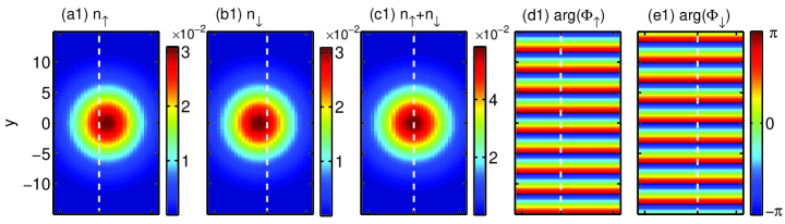
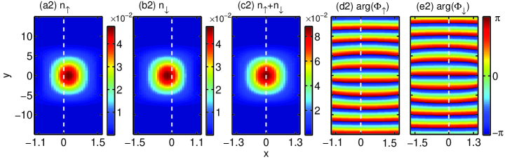
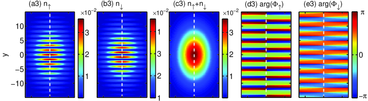
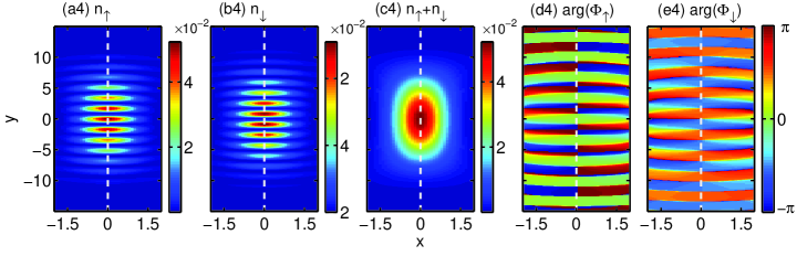
Figure 1: (Color online) Profiles of the density $n_{\uparrow,\downarrow}=|\Phi_{\uparrow,\downarrow}|^{2}$ of spin $\uparrow$ ($\downarrow$) in (a)((b)), the total density $n_{\uparrow}+n_{\downarrow}$ in (c), the phase of spin $\uparrow$($\downarrow$) in (d)((e)) for a plane wave soliton (the first two panels) with $\gamma_{12}=6$ and a stripe soliton (the last two panels) with $\gamma_{12}=10$. The solitons in the first and third panels are obtained by the variational method, while the solitons in the second and forth panels are calculated by the imaginary time evolution of the GP Eq. (11). The dashed white line labels the $x=0$ line. Here, $\gamma=8$, $\gamma_{d}/\gamma=0.67$, and $\alpha=2$.

III Stationary bright solitons

To shed light on the structure of a soliton, we start from the homogeneous noninteracting single particle scenario and write its momentum space dispersion as

$$E({\bf k})=\frac{{\bf k}^{2}}{2}\pm\alpha k,$$ (15)

with two branches labeled by the helicity $\pm$. Clearly, the ground state is degenerate with the energy being $-\alpha^{2}/2$ when the momenta lie in the $k=|\alpha|$ ring. This is different from the case without spin-orbit coupling where the ground state only occurs at $k=0$. In this single particle case, any superposition of the states in the ring is also its ground state. Yet, this is not the case when the repulsive contact interaction is involved. The ground state either possesses a single momentum (i.e. plane wave phase) when $\gamma_{12}/\gamma<1$ or two opposite momenta (i.e. stripe phase) when $\gamma_{12}/\gamma>1$ ZhaiHui2010PRL . When the dipolar interaction is turned on, one may expect that this effective long ranged attractive interaction along with contact repulsive interaction could support two types of solitons: plane wave and stripe solitons.

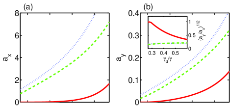
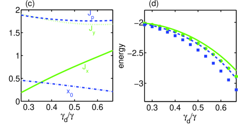
Figure 2: (Color online) Plot of $a_{x}$ in (a) and $a_{y}$ in (b) as a function of $\gamma_{d}/\gamma$ for the plane wave solitons (dotted blue line), stripe solitons (dashed green line), and traditional solitons (solid red line) without spin-orbit coupling. The aspect ratio $\sqrt{a_{y}/a_{x}}$ of a soliton is displayed in the inset of (b). Variational parameters with respect $\gamma_{d}/\gamma$ are plotted in (c) associated with $x_{0}$ (dash-dot blue line) and $J_{p}$ (dashed blue line) for the plane wave soliton, and $J_{x}$ (solid green) and $J_{y}$ (dotted green) for the stripe soliton. In (d), the total energy of the variational ansatz wave function and the wave function numerically obtained by the imaginary time evolution of the GPE for both plane wave and stripe solitons is shown. The solid green line (stripe soliton) and dashed blue line (plane wave soliton) correspond to the variational results, while the green circles and blue squares correspond to the GP results. Here, $\alpha=2$, $\gamma=8$, $\gamma_{12}=6$ ($\gamma_{12}=10$) for the plane wave (stripe) soliton.

To examine whether a soliton can indeed exist in the spin-orbit-coupled dipolar BECs, we first consider a plane wave soliton variational ansatz

$${\Phi_{P}}=\begin{pmatrix}\Phi_{0}(x_{0}/2)\\ -\Phi_{0}(-x_{0}/2)\end{pmatrix}\text{exp}(-iJ_{p}y),$$ (16)

where

$$\Phi_{0}(x_{0})=\frac{(a_{x}a_{y})^{1/4}}{\sqrt{2\pi}}e^{-\frac{1}{2}[a_{x}(x-x_{0})^{2}+a_{y}y^{2}]}.$$ (17)

Here $J_{p}$ is the wave vector of the plane wave soliton, $l_{\nu}=1/\sqrt{a_{\nu}}$ with $\nu=x,y$ is the size of the soliton, and $x_{0}$ is the separation distance between two components. When $x_{0}=0$, this state is an eigenstate of $p_{y}\sigma_{x}$ multiplied by a Gaussian profile $\Phi_{0}(0)$, and $J_{p}=\alpha$ yields the minimum energy. In fact, $x_{0}$ is usually nonzero because of a force acting on the BEC by spin-orbit coupling $\bf{F}=\alpha^{2}({\bf p}\times{\bf e}_{z})\sigma_{z}$ Yongping2012PRL ; Shuwei2013JPB , which is opposite along the $x$ direction when $\bf p$ (here $J_{p}$) is along the $y$ direction.

In writing down the ansatz (16), we have assumed that the wave vector $J_{p}$ is in the $y$ direction. The prerequisite of this assumption is that the rotation symmetry Yongping2012PRL ; Hu2012PRL about the $z$ axis has been broken by the dipole-dipole interaction. Indeed, without the dipole-dipole interaction, this state with $J_{p}$ along $y$ is not special and other states with $J_{p}$ along other directions are degenerate with it. For example, the state with $J_{p}$ along $y$ has the same energy as a state with $J_{p}$ along $x$. Yet, with the specific dipole-dipole interaction arising from the dipoles entirely oriented along $y$, the symmetry is broken and the ground state should be elongated along $y$ ($a_{x}>a_{y}$) so as to provide an effective attractive interaction because of the head-to-tail configuration of polarized dipoles. This elongated configuration allows the existence of a 2D soliton Malomed2008PRL and also requires the wave vector to be along $y$ note1 .

Although the wave vector $J_{p}$ of the ground state is along $y$, there are still two options: negative and positive directions in terms of the time-reversal symmetry $\mathcal{T}$ (i.e. $-i\sigma_{y}\mathcal{K}$ with the complex conjugate operator $\mathcal{K}$). Specifically, the state $\Phi_{P2}=\mathcal{T}\Phi_{P}$ is degenerate with $\Phi_{P}$. In the absence of interactions, all superposition states of $\Phi_{P}$ and $\Phi_{P2}$,

$$\Phi_{PS}=|\cos\theta|\Phi_{P}+|\sin\theta|e^{i\varphi}\Phi_{P2},$$ (18)

are degenerate. This degeneracy may be broken by the interaction so that the ground state is either $\Phi_{P}$ or $\Phi_{P2}$, or a certain superposition state of them. But this degeneracy breaking should not happen at $\gamma_{12}/\gamma=1$ since the interaction energy only depends on the total density which is independent of $\theta$ and $\varphi$. This gives us an intuitive understanding that $\gamma_{12}/\gamma=1$ may separate the plane wave soliton ($|\cos\theta|=$0 or 1) and the stripe soliton ($|\cos\theta|=|\sin\theta|$), similar to the homogenous spin-orbit-coupled BEC ZhaiHui2010PRL without dipole-dipole interactions. For the stripe soliton, we note that $\varphi=0,\pi$ corresponds to the ground state as the energy contributed by $\varphi$ is $-\gamma_{12}\sqrt{a_{x}a_{y}}e^{-(a_{x}x_{0}^{2}/2+2J_{p}^{2}/a_{y})}\cos(2\varphi)/(16\pi)$  ExplainVarphi .

To evaluate the variational parameters $a_{x}$, $a_{y}$, $x_{0}$, $J_{p}$, and $\theta$, we minimize the energy $\mathcal{E}$ after substituting $\Phi_{PS}$ in Eq. (18) to Eq. (10). Indeed, the calculated variational solutions reveal that there are two types of soliton solutions: plane wave solitons when $\gamma_{12}/\gamma<1$ and stripe solitons when $\gamma_{12}/\gamma>1$. We present the density and phase profiles of a typical plane wave soliton (we choose $\theta=\varphi=0$) in the first panel of Fig. 1, where the stripe structure of the phase of both two components reveals the plane wave feature. The soliton is highly elongated along the $y$ direction and the centers of two components are spatially separated along the $x$ direction because of nonzero $x_{0}$. To confirm that this variational solution can qualitatively characterize the ground state of the system, we numerically compute the ground state by an imaginary time evolution of the GP Eq. (11). This exact numerical solution also concludes that $\gamma_{12}/\gamma<1$ yields the plane wave soliton while $\gamma_{12}/\gamma>1$ the stripe soliton. In the second panel of Fig. 1, we also plot the corresponding density and phase profiles of the GP obtained plane wave soliton. The variational ansatz is in qualitative agreement with it given the separated centers and the plane wave varying phase that both states possess. Yet, the shape of the soliton obtained by the imaginary time evolution deviates slightly from the Gaussian and the size is also slightly smaller.

When $\theta=\pi/4$ and $\varphi=0$, $\Phi_{PS}$ is a stripe state with a density oscillation along the $y$ direction for each component. And there is no stripe for the total density. Along the $x$ direction, two components are not spatially separated, and the phase for the spin $\uparrow$ reverses suddenly across $x=0$. Following these properties by replacing $(\Phi_{0}(x_{0}/2)+\Phi_{0}(-x_{0}/2))/\sqrt{2}$ with $\cos(J_{x}x)\Phi_{0}(0)$ and $(\Phi_{0}(x_{0}/2)-\Phi_{0}(-x_{0}/2))/\sqrt{2}$ with $\sin(J_{x}x)\Phi_{0}(0)$ in Eq. (18), we obtain another better variational ansatz for the stripe soliton

$$\Phi_{S}=\Gamma\Phi_{0}(0),$$ (19)

where

$$\Gamma=\begin{pmatrix}\cos(J_{y}y)\cos(J_{x}x)-i\sin(J_{y}y)\sin(J_{x}x)\\ \cos(J_{y}y)\sin(J_{x}x)+i\sin(J_{y}y)\cos(J_{x}x)\end{pmatrix},$$ (20)

with the variational parameters $J_{x}$ and $J_{y}$. The period of the stripe along the $y$ direction is $\pi/J_{y}$. Interestingly, this stripe soliton corresponds to four points $(\pm J_{x},\pm J_{y})$ in momentum space instead of traditional two points Yong2013PRA when $J_{x}=0$, if we do not consider the Gaussian profile $\Phi_{0}$.

We calculate the variational parameters of stripe solitons by performing the minimization of the energy $\mathcal{E}$ in Eq. (10) where $\Phi$ is replaced with $\Phi_{S}$. The density and phase profiles of a typical stripe soliton calculated by this method is displayed in the third panel of Fig. 1. Evidently, the density of each component exhibits the stripe structure while the total density does not. The phase of spin $\uparrow$ along the $y$ direction varies like a plane wave, but reverses across $x=0$ due to the presence of $\sin(J_{x}x)$ in the imaginary part. The phase of spin $\downarrow$ exhibits the phase rotation like vortices around $x=0$ and $y=n\pi/J_{y}$ with integer $n$; around these points, the wave function $\Phi_{S\downarrow}$ is proportional to $(-1)^{n}(J_{x}x+i(J_{y}y-n\pi))$ and the corresponding density of spin $\downarrow$ is extremely low. Moreover, in the last panel of Fig. 1, we plot the density and phase profiles of the corresponding stripe soliton obtained by the imaginary time evolution of the GPE; comparing this figure with the third panel of Fig. 1 implies that the stripe variational ansatz is qualitatively consistent with the GP results.

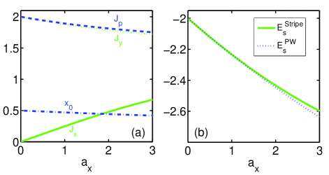
Figure 3: (Color online) Plot of $x_{0}$ (dash-dot blue line) and $J_{p}$ (dashed blue line) for the plane wave variational ansatz, and $J_{x}$ (solid green line) and $J_{y}$ (dotted green line) for the stripe variational ansatz with respect to $a_{x}$ by the minimization of the energy $E_{s}^{\rm PW}$ and $E_{s}^{\rm Stripe}$ in (a). (b) shows the minimum energy of $E_{s}^{\rm PW}$ (dotted blue line) and $E_{s}^{\rm Stripe}$ (solid green line) as a function of $a_{x}$. Here, $\alpha=2$.

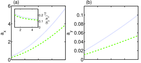
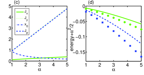
Figure 4: (Color online) Plot of $a_{x}$ in (a) and $a_{y}$ in (b) as a function of the spin-orbit coupling strength $\alpha$ for the plane wave soliton (dotted blue line) and stripe soliton (dashed green line). The aspect ratio $\sqrt{a_{y}/a_{x}}$ of a soliton is plotted in the inset of (a). (c) illustrates the change of $x_{0}$ (dash-dot blue line), $J_{p}$ (dashed blue line) for the plane wave soliton and $J_{x}$ (solid green line) and $J_{y}$ (dotted green line) for the stripe soliton with respect to $\alpha$. In (d), the total energy plus $\alpha^{2}/2$ is plotted as a function of $\alpha$. The solid green (for a stripe soliton) and dashed blue (for a plane wave soliton) are calculated by the variational method, while the green circles (for a stripe soliton) and blue squares (for a plane wave soliton) are numerically obtained by the imaginary time evolution of the GPE. Here, $\gamma=8$, $\gamma_{d}/\gamma=0.67$, and $\gamma_{12}=6$ ($\gamma_{12}=10$) for the plane wave (stripe) soliton.

To study the properties of a soliton with respect to dipole-dipole interactions $\gamma_{d}$, we evaluate the variational parameters of both the plane wave and stripe solitons by the variational method and plot them in Fig. 2 as $\gamma_{d}/\gamma$ varies. Clearly, with increasing $\gamma_{d}/\gamma$, $a_{x}$ and $a_{y}$ increase monotonously because of the enhanced effective attractive interaction, indicating that the size $l_{x}$ and $l_{y}$ of the soliton decrease monotonously. We note that as $\gamma_{d}/\gamma$ increases further, the soliton can collapse so that both $a_{x}$ and $a_{y}$ diverge. For the plane wave soliton, $a_{x}$ and $a_{y}$ are slightly larger than the stripe soliton because of the smaller contact interaction of the former. Moreover, compared with the soliton without spin-orbit coupling (red line in Fig. 2(a) and (b)), $a_{x}$ and $a_{y}$ for both the plane wave and stripe solitons are much larger, implying that the size of solitons can be reduced by spin-orbit coupling. Also, these solitons are highly anisotropic with the much smaller aspect ratio $\sqrt{a_{y}/a_{x}}$ as shown in the inset of Fig. 2(b). To elucidate the reason, we explicitly write that single particle energy of the plane wave variational ansatz in Eq.(16) which results from the presence of $x_{0}$ and $J_{p}$

$$E_{s}^{\rm PW}=\frac{1}{2}J_{p}^{2}-\alpha e^{-\frac{x_{0}^{2}a_{x}}{4}}(J_{p}+\frac{1}{2}a_{x}x_{0}).$$ (21)

The minimization of $E_{s}^{\rm PW}$ with respect to $x_{0}$ and $J_{p}$ for fixed $a_{x}$ yields

$$x_{0} = \frac{-J_{p}+\sqrt{J_{p}^{2}+2a_{x}}}{a_{x}}$$ (22)

$$J_{p} = \alpha e^{-x_{0}^{2}a_{x}/4}.$$ (23)

For $a_{x}=0$, the energy is independent of $x_{0}$ and $J_{p}=\alpha$, while for $a_{x}\neq 0$, both $x_{0}$ and $J_{p}$ decrease slightly with increasing $a_{x}$ as shown in Fig. 3(a) with the asymptotic $x_{0}=1/\alpha$ and $J_{p}=\alpha$ as $a_{x}$ goes zero. The energy $E_{s}^{PW}$ is also a monotonously decreasing function of $a_{x}$. And this energy decline combined with the reduced dipole-dipole interaction energy competes with the rise of the kinetic energy (when $x_{0}=J_{p}=0$) and contact interaction energy, leading to an increased $a_{x}$ and $a_{y}$ compared with the soliton without spin-orbit coupling. This is also consistent with Fig. 2(c), showing that with increasing the dipole-dipole interaction, $a_{x}$ increases and both $x_{0}$ and $J_{p}$, therefore, decrease so as to lower $E_{s}^{\rm PW}$. It is important to note that although $E_{s}^{\rm PW}$ is not a function of $a_{y}$, other energy such as the kinetic energy (when $x_{0}=J_{p}=0$), the contact and dipolar interaction energy depends on it.

For the stripe soliton, the single particle energy due to the presence of $J_{x}$ and $J_{y}$ is

$$E_{s}^{\rm Stripe}=\frac{1}{2}(J_{x}^{2}+J_{y}^{2})-\alpha(J_{x}+J_{y}e^{-J_{x}^{2}/a_{x}}).$$ (24)

Similar to the plane wave case, this energy is independent of $a_{y}$. For fixed $a_{x}$, the minimization of this energy yields both $J_{x}$ and $J_{y}$ as a function of $a_{x}$ as shown in Fig. 3(a). When $a_{x}$ moves towards zero, the solution approaches ($J_{x}=\alpha$, $J_{y}=0$) or ($J_{x}=0$, $J_{y}=\alpha$); when it moves away from zero, there is only one solution where $J_{y}$ decreases from $\alpha$ while $J_{x}$ increases from zero with the rise of $a_{x}$. Also, the energy $E_{s}^{\rm Strip}$ decreases as $a_{x}$ increases. Analogous to the plane wave soliton, the total energy decrease resulted from spin-orbit coupling and dipole-dipole interactions as $a_{x}$ and $a_{y}$ increase from the value without spin-orbit coupling exceeds the energy gain of the kinetic (when $J_{x}=0$ and $J_{y}=0$) and contact interaction; this leads to the increased $a_{x}$ and $a_{y}$ compared with the soliton without spin-orbit coupling. This picture is also consistent with Fig. 2(c) where $J_{x}$ increases while $J_{y}$ decreases with respect to $\gamma_{d}/\gamma$.

To explicitly demonstrate the effect of the spin-orbit coupling on the properties of a soliton, we plot the variational parameters as a function of the spin-orbit coupling strength $\alpha$ for both the plane wave and stripe solitons in Fig. 4. Consistent with the aforementioned feature that spin-orbit coupling can reduce the size of the soliton, both Fig. 4(a) and Fig. 4(b) display a monotonous increasing behavior of $a_{x}$ and $a_{y}$ as a function of $\alpha$. Also, the aspect ratio $\sqrt{a_{y}/a_{x}}$ is decreased by spin-orbit coupling. Similar to Fig. 2(a) and Fig. 2(b), $a_{x}$ and $a_{y}$ for the plane wave soliton are slightly larger than the stripe soliton in that the former has a smaller contact interaction. For the plane wave soliton, $J_{P}$ (determined mainly by the spin-orbit coupling strength) increases with respect to $\alpha$ while $x_{0}$ decreases; for the stripe soliton, both $J_{x}$ and $J_{y}$ increase.

In Fig. 2(d) and Fig. 4(d), for both plane wave and stripe solitons, we compare their energy obtained by the variational procedure with the one obtained by the imaginary time evolution of the GPE. Both figures show that the energy calculated by the imaginary time evolution is lower as expected. Yet, the difference between these two energy is not large (no more than 10%), suggesting that the variational ansatz can qualitatively characterize the solitons. We note that in Fig. 4(d), the energy is shifted by $\alpha^{2}/2$ in order to clearly present the different results of the two methods, which could be smeared by the large value of $\alpha^{2}/2$.

IV Moving bright solitons

Generally, the wave function of a moving soliton with the velocity ${\bf v}$ can be simply written as $\exp(i{\bf v}\cdot{\bf r})\Phi_{s}({\bf r}-{\bf v}t)$ where $\Phi_{s}$ is the wave function of a stationary soliton. But this is only valid for a system respecting Galilean transform invariance. In fact, Galilean invariance is broken in a spin-orbit-coupled BEC Qizhong2013 , and this violation dictates that the shape of a soliton depends on its velocity strength Yong2013PRA . Here, for a soliton in a spin-orbit-coupled dipolar BEC in 2D, we assume that a moving soliton can be written as

$${\Phi_{M}}({\bf r},t)=\Phi_{v}({\bf r}-{\bf v}t,t)\exp({i{\bf v}\cdot{\bf r}-i\frac{1}{2}v^{2}t}),$$ (25)

where $\Phi_{v}$ is a localized function. Plugging ${\Phi_{M}}({\bf r},t)$ into Eq. (11) yields

$$i\frac{\partial\Phi_{v}({\bf r})}{\partial t}= \mathcal{H}_{s}({\bf v})\Phi_{v}({\bf r})+\gamma\mathcal{G}\Phi_{v}({\bf r})$$ (26)

$$+\gamma_{d}\int d{\bf k}e^{i{\bf k}\cdot{\bf r}}n({\bf k})U_{d}({\bf k})\Phi_{v}({\bf r}),$$

where $\mathcal{H}_{s}({\bf v})=\mathcal{H}_{s}+\alpha({\bf v}\times{\bm{\sigma}})\cdot{\bf e}_{z}$. Compared to Eq. (11), this dynamical equation has an additional term $\alpha({\bf v}\times{\bm{\sigma}})\cdot{\bf e}_{z}$, acting as a Zeeman field; this additional term implies the violation of Galilean invariance. This violation means that it is no longer a trivial task to find a moving bright soliton for a BEC with spin-orbit coupling; we need to perform an imaginary time evolution of the Eq. (26), but not Eq. (11). Furthermore, such a 2D moving soliton should be different for different velocity directions even if their amplitude is the same, in contrast to a 1D soliton which can only move in one direction.

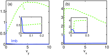
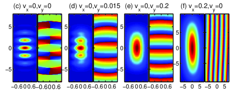
Figure 5: (Color online) Imbalance $Imb$ and width $l_{x}$ of spin $\uparrow$ of the solitons with respect to the velocity along the $y$ ($x$) direction in (a) ((b)). The insets display the enlarged figure in a small velocity region. Density and phase profiles of four typical moving solitons for spin $\uparrow$ corresponding to the different velocities in (a) and (b) are plotted in (c-f) where the horizontal and vertical coordinates are $x$ and $y$ respectively. Here, $\alpha=2$, $\gamma=8$, $\gamma_{12}=10$, and $\gamma_{d}/\gamma=1$, corresponding to a stripe soliton when stationary.

To examine how the shape of a soliton changes with respect to the velocities along $x$ and $y$ directions, we plot the imbalance $Imb$ and the width $l_{x}$ of a soliton of spin $\uparrow$ as a function of the velocities $v_{x}$ and $v_{y}$ in Fig. 5. Here, the imbalance for spin $\uparrow$ is defined as

$$Imb=\frac{|\Phi_{\uparrow}(0)|^{2}-|\Phi_{\uparrow}(\pi/(2\alpha))|^{2}}{|\Phi_{\uparrow}(0)|^{2}+|\Phi_{\uparrow}(\pi/(2\alpha))|^{2}},$$ (27)

which characterizes a stripe soliton (as shown in Fig. 5(c) and Fig. 5(d)) when it approaches one and a plane wave soliton (as shown in Fig. 5(e) and Fig. 5(f)) when it approaches zero. Fig. 5(a) and Fig. 5(b) demonstrate that $Imb$ suffers a sharp decline from one to near zero as $v_{x}$ and $v_{y}$ increase, indicating that a moving soliton tends to be a plane wave state. The reason is the broken rotation symmetry of the single particle Hamiltonian by the velocity induced Zeeman field, giving rise to a ground state of the single particle system lying at one momentum point located along the $x$ ($y$) direction when the velocity is along that direction. This also explains why the phase of a moving plane wave soliton with the velocity along the $x$ ($y$) direction varies along that direction.

Furthermore, Fig. 5(a) demonstrates that the width of the soliton gradually grows when the velocity along the $y$ direction is enlarged, To explain the growth, we consider the plane wave ansatz in Eq. (16) which yields an additional term $-\alpha v_{y}e^{-a_{x}x_{0}^{2}/4}$ for the single particle energy when a soliton moves; this energy decrease enlarges exponentially with the decline of $a_{x}$ (i.e. increase of the width), leading to an expanded soliton with the rise of the velocity. However, this is not a monotonous behavior and the soliton begins shrinking when the velocity goes larger, due to the enlarged $J_{p}$ by the velocity induced Zeeman field, similar to increasing spin-orbit coupling. On the other hand, when the velocity is along the $x$ direction, the width of the soliton gains a sudden rise as the velocity varies, as shown Fig. 5(b). This corresponds to a change from a stripe soliton with the wave vector along the $y$ direction to a plane wave soliton with the wave vector along the $x$ direction. For the stationary solitons, the soliton with the wave vector mainly along the $y$ direction has lower energy than the one with the wave vector mainly along the $x$ direction as the dipoles are completely oriented along $y$. But the Zeeman field induced by the presence of a velocity along the $x$ direction gives rise to the single particle ground state that possesses the wave vector along $x$. The two states with the wave vector along these two directions compete and change from the former to the latter (i.e. first order phase transition). For the decrease of the width when $v_{x}$ goes even larger, the reason is the same as the case for $v_{y}$. When a stationary soliton is plane wave, the moving behavior is similar except that the moving soliton is always the plane wave soliton.

V Conclusion

We have studied the bright solitons as the ground states in a spin-orbit-coupled dipolar BEC in 2D with dipoles completely polarized along one direction in the 2D plane. It is important to note that the solitons are the ground states in 2D, but they are the metastable states in quasi-2D where the true ground state would collapse and there is an energy barrier between the soliton state and this ground state. Two types of solitons have been found: a plane wave soliton and a stripe soliton. The former has the plane wave phase variation and its two components are slightly spatially separated; while for the latter, the density of each component is spatially oscillating and the variational ansatz suggests that four points in momentum space are involved. Both plane wave and stripe solitons are highly anisotropic and their size is decreased by spin-orbit coupling. These solitons cannot exist as the ground states in a 2D system with pure attractive contact interactions and spin-orbit coupling. Moreover, the shape of these solitons changes with their velocities due to the absence of Galilean invariance, and this change is anisotropic.

The 2D bright soliton, albeit mainly plane wave soliton, can also exist when equal Rashba and Dresselhaus spin-orbit coupling is considered. In experiments, this type of spin-orbit coupling has been engineered by coupling two hyperfine states of atoms through two counterpropagating Raman laser beams Lin2011Nature ; Jing2012PRL ; Zwierlen2012PRL ; PanJian2012PRL ; Peter2013 ; Spilman2013PRL and such setup could be employed to realize this spin-orbit coupling in Dysprosium Cui2013PRA with large dipole-dipole interactions. Also, the large magnetic moment in Dysprosium atoms may permit the realization of Rashba spin-orbit coupling Spielman2011PRA .

- (1) C. J. Pethick and H. Smith, Bose-Einstein Condensation in Dilute Gases, 2nd ed. (Cambridge University Press, Cabmridge, 2008).
- (2) P. G. Kevrekidis, D. J. Frantzeskakis, and R. Carretero-González, Emergent Nonlinear Phenomena in Bose-Einstein Condensates, Springer, 2007.
- (3) C. Chin, R. Grimm, P. Julienne, and E. Tiesinga, Rev. Mod. Phys. 82, 1225 (2010).
- (4) S. Burger, K. Bongs, S. Dettmer, W. Ertmer, K. Sengstock, A. Sanpera, G. V. Shlyapnikov, and M. Lewenstein, Phys. Rev. Lett. 83, 5198 (1999).
- (5) J. Denschlag, J. E. Simsarian, D. L. Feder, C. W. Clark, L. A. Collins, J. Cubizolles, L. Deng, E. W. Hagley, K. Helmerson, W. P. Reinhardt, S. L. Rolston, B. I. Schneider, and W. D. Phillips, Science 287, 97 (2000).
- (6) B. P. Anderson, P. C. Haljan, C. A. Regal, D. L. Feder, L. A. Collins, C. W. Clark, and E. A. Cornell, Phys. Rev. Lett. 86, 2926 (2001).
- (7) K. E. Strecker, G. B. Partridge, A. G. Truscott, and R. G. Hulet, Nature (London) 417, 150 (2002).
- (8) L. Khaykovich, F. Schreck, G. Ferrari, T. Bourdel, J. Cubizolles, L. D. Carr, Y. Castin, and C. Salomon, Science 296, 1290 (2002).
- (9) S. L. Cornish, S. T. Thompson, and C. E. Wieman, Phys. Rev. Lett. 96, 170401 (2006).
- (10) B. Eiermann, Th. Anker, M. Albiez, M. Taglieber, P. Treutlein, K.-P. Marzlin, and M. K. Oberthaler, Phys. Rev. Lett. 92, 230401 (2004).
- (11) C. Hamner, Y. Zhang, J. J. Chang, C. Zhang, and P. Engels, Phys. Rev. Lett. 111, 264101 (2013).
- (12) J. H. V. Nguyen, P. Dyke, D. Luo, B. A. Malomed, and R. G. Hulet. Nat. Phys. 10, 918 (2014).
- (13) Both the kinetic energy and the contact attractive interaction energy in 2D is proportial to with the size of a state; to lower energy, the state collapses (i.e. ) when the interaction energy is larger than the kinetic one, and the state expands (i.e. ) otherwise.
- (14) W. Krolikowski, O. Bang, J. J. Rasmussen, and J. Wyller, Phys. Rev. E 64, 016612 (2001).
- (15) T. Lahaye, C. Menotti, L. Santos, M. Lewenstein, and T. Pfau, Rep. Prog. Phys. 72, 126401 (2009).
- (16) P. Pedri and L. Santos, Phys. Rev. Lett. 95, 200404 (2005).
- (17) I. Tikhonenkov, B. A. Malomed, and A. Vardi, Phys. Rev. Lett. 100, 090406 (2008).
- (18) C. Ticknor, R. M. Wilson, and J. L. Bohn, Phys. Rev. Lett. 106, 065301 (2011).
- (19) M. A. Baranov, M. Dalmonte, G. Pupillo, and P. Zoller, Chem. Rev. 112, 5012 (2012).
- (20) A. Griesmaier, J. Werner, S. Hensler, J. Stuhler, and T. Pfau, Phys. Rev. Lett. 94, 160401 (2005).
- (21) T. Koch, T. Lahaye, J. Metz, B. Frhlich, A. Griesmaier, and T. Pfau, Nat. Phys. 4, 218 (2008).
- (22) Q. Beaufils, R. Chicireanu, T. Zanon, B. Laburthe-Tolra, E. Maréhal, L. Vernac, J.-C. Keller, and O. Gorceix, Phys. Rev. A 77, 061601(R) (2008).
- (23) M. Lu, N. Q. Burdick, S. H. Youn, and B. L. Lev, Phys. Rev. Lett. 107, 190401 (2011).
- (24) K. Aikawa, A. Frisch, M. Mark, S. Baier, A. Rietzler, R. Grimm, and F. Ferlaino, Phys. Rev. Lett. 108, 210401 (2012).
- (25) M. Lu, N. Q. Burdick, and B. L. Lev, Phys. Rev. Lett. 108, 215301 (2012).
- (26) K. Aikawa, A. Frisch, M. Mark, S. Baier, R. Grimm, and F. Ferlaino, Phys. Rev. Lett. 112, 010404 (2014).
- (27) Y. -J. Lin, K. Jiménez-García, and I. B. Spielman, Nature (London) 471, 83 (2011).
- (28) P. Wang, Z. -Q. Yu, Z. Fu, J. Miao, L. Huang, S. Chai, H. Zhai, and J. Zhang, Phys. Rev. Lett. 109, 095301 (2012).
- (29) L. W. Cheuk, A. T. Sommer, Z. Hadzibabic, T. Yefsah, W. S. Bakr, and M. W. Zwierlein, Phys. Rev. Lett. 109, 095302 (2012).
- (30) J. -Y. Zhang, S. -C. Ji, Z. Chen, L. Zhang, Z. -D. Du, B. Yan, G. -S. Pan, B. Zhao, Y. -J. Deng, H. Zhai, S. Chen, and J. -W. Pan, Phys. Rev. Lett. 109, 115301 (2012).
- (31) C. Qu, C. Hamner, M. Gong, C. Zhang, and P. Engels, Phys. Rev. A 88, 021604(R) (2013).
- (32) R. A. Williams, M. C. Beeler, L. J. LeBlanc, K. Jiménez-García, and I. B. Spielman, Phys. Rev. Lett. 111, 095301 (2013).
- (33) T. D. Stanescu, B. Anderson, and V. Galitski, Phys. Rev. A 78, 023616, (2008).
- (34) C. Wang, C. Gao, C.-M. Jian, H. Zhai, Phys. Rev. Lett. 105, 160403 (2010).
- (35) C. Wu, I. Mondragon-Shem, and X. F. Zhou, Chin. Phys. Lett. 28, 097102 (2011)
- (36) T. -L. Ho and S. Zhang, Phys. Rev. Lett. 107, 150403 (2011).
- (37) S. Sinha, R. Nath, and L. Santos, Phys. Rev. Lett. 107, 270401 (2011).
- (38) Y. Zhang, L. Mao, and C. Zhang, Phys. Rev. Lett. 108, 035302 (2012).
- (39) H. Hu, B. Ramachandhran, H. Pu, and X. J. Liu, Phys. Rev. Lett. 108, 010402 (2012).
- (40) Y. Li, L. P. Pitaevskii, and S. Stringari, Phys. Rev. Lett. 108, 225301 (2012).
- (41) Z. Chen and H. Zhai, Phys. Rev. A 86, 041604(R) (2012).
- (42) K. Sun, C. Qu, and C. Zhang, arXiv:1411.1737.
- (43) Y. Xu, F. Zhang, and C. Zhang, arXiv:1411.7316.
- (44) J. Dalibard, F. Gerbier, G. Juzeliunas, and P. Öhberg, Rev. Mod. Phys. 83, 1523 (2011).
- (45) V. Galitski and I. B. Spielman, Nature (London) 494, 49 (2013).
- (46) X. Zhou, Y. Li, Z. Cai, and C. Wu, J. Phys. B: At. Mol. Opt. Phys. 46 134001 (2013).
- (47) N. Goldman, G. Juzeliūnas, P. Öhberg, and I. B. Spielman, Rep. Prog. Phys. 77 126401 (2014).
- (48) H. Zhai, Rep. Prog. Phys. 78 026001 (2015).
- (49) W. Yi, W. Zhang, and X. Cui, Science China Physics Mechanis & Astronomy, 58, 1 (2014).
- (50) J. Zhang, H. Hu, X.-J. Liu, and H. Pu, Ann. Rev. Cold At. Mol. 2, 81 (2014).
- (51) Y. Xu and C. Zhang, Int. J. Mod. Phys. B 28, 1530001 (2015).
- (52) M. Merkl, A. Jacob, F. E. Zimmer, P. Öhberg, and L. Santos, Phys. Rev. Lett. 104, 073603 (2010).
- (53) Y. Xu, Y. Zhang, and B. Wu, Phys. Rev. A 87, 013614 (2013).
- (54) V. Achilleos, D. J. Frantzeskakis, P. G. Kevrekidis, D. E. Pelinovsky, Phys. Rev. Lett. 110, 264101 (2013).
- (55) L. Salasnich and B. A. Malomed, Phys. Rev. A 87, 063625 (2013).
- (56) H. Sakaguchi and B. A. Malomed, Phys. Rev. E 90, 062922 (2014).
- (57) L. Salasnich, W. B. Cardoso, and B. A. Malomed, Phys. Rev. A 90, 033629 (2014).
- (58) H. Sakaguchi, B. Li, and B. A. Malomed, Phys. Rev. E 89, 032920 (2014).
- (59) O. Fialko, J. Brand, and U. Zülicke, Phys. Rev. A 85, 051605(R) (2012).
- (60) V. Achilleos, J. Stockhofe, P. G. Kevrekidis, D. J. Frantzeskakis, and P. Schmelcher, Europhys. Lett. 103, 20002 (2013).
- (61) Y. V. Kartashov, V. V. Konotop, and F. K. Abdullaev, Phys. Rev. Lett. 111, 060402 (2013).
- (62) V. E. Lobanov, Y. V. Kartashov, and V. V. Konotop, Phys. Rev. Lett. 112, 180403 (2014).
- (63) Y. Zhang, Y. Xu, and T. Busch, arXiv:1502.04409.
- (64) Y. Xu, L. Mao, B. Wu, and C. Zhang, Phys. Rev. Lett. 113, 130404 (2014).
- (65) X.-J. Liu, Phys. Rev. A 91, 023610(2015).
- (66) Q. Zhu, C. Zhang, and B. Wu, Europhys. Lett. 100, 50003 (2013).
- (67) Q. Zhu and B. Wu, arXvi:1501.04153.
- (68) Y. Deng, J. Cheng, H. Jing, C. -P. Sun, and S. Yi, Phys. Rev. Lett. 108, 125301 (2012).
- (69) X. Cui, B. Lian, T.-L. Ho, B. L. Lev, and H. Zhai, Phys. Rev. A 88, 011601(R) (2013).
- (70) H. T. Ng, Phys. Rev. A 90, 053625 (2014).
- (71) Y. Yousefi, E. Ö. Karabulut, F. Malet, J. Cremon, S. M. Reimann, arXiv:1412.0505.
- (72) S. Gopalakrishnan, I. Martin, E. A. Demler, Phys. Rev. Lett. 111, 185304 (2013).
- (73) R. M. Wilson, B. M. Anderson, and C. W. Clark, Phys. Rev. Lett. 111, 185303 (2013).
- (74) S. -W. Song, Y. -C. Zhang, L. Wen, and H. Wang, J. Phys. B: At. Mol. Opt. Phys. 46 145304 (2013).
- (75) This elongated configuration along with the wave vector in the direction has the lower single particle energy contributed by the spin-orbit coupling than the case with the wave vector in the direction.
- (76) This energy is generally so small that the states with different are nearly degenerate. That might be the reason why the stripe state for which possesses a sharp phase change across the symmetric axis in a harmonically trapped spin-orbit-coupled BEC has not been noticed Yongping2012PRL .
- (77) D. L. Campbell, G. Juzeliūnas, and I. B. Spielman, Phys. Rev. A 84, 025602 (2011).