Straight-line Drawability of a
Planar Graph Plus an Edge

Abstract

We investigate straight-line drawings of topological graphs that consist of a planar graph plus one edge, also called almost-planar graphs. We present a characterization of such graphs that admit a straight-line drawing. The characterization enables a linear-time testing algorithm to determine whether an almost-planar graph admits a straight-line drawing, and a linear-time drawing algorithm that constructs such a drawing, if it exists. We also show that some almost-planar graphs require exponential area for a straight-line drawing.

1 Introduction

This paper investigates straight-line drawings of almost-planar graphs, that is, graphs that become planar after the deletion of just one edge.

Our work is partly motivated by the classical planarization approach [1] to graph drawing. This method takes as input a graph $G$, deletes a small number of edges to give a planar subgraph $G^{-}$, and then constructs a planar topological embedding (i.e., a plane graph) of $G^{-}$. Then the deleted edges are re-inserted, one by one, to give a topological embedding of the original graph $G$. Finally, a drawing algorithm is applied to the topological embedding. A number of variations on this basic approach give a number of graph drawing algorithms (see, e.g., [1]). This paper is concerned with the final step of creating a drawing from the topological embedding.

Minimizing the number of edge crossings is an NP-hard problem even when the given graph is almost-planar [3]. However, Gutwenger, Mutzel, and Weiskircher [7] present an elegant polynomial-time solution to the following simpler problem: Given a graph $G$ and an edge $e$ such that $G^{-}=G-e$ is planar, find a planar topological embedding of $G^{-}$ that minimizes the number of edge crossings when re-inserting $e$ in $G$.

While the output of the algorithm of Gutwenger et al. has the minimum number of edge crossings, it may not give rise to a straight-line planar drawing. In this paper we study the following problem: Let $G$ be a topological graph consisting of a planar graph plus an edge $e$. We want to test whether $G$ admits a straight-line drawing that preserves the given embedding.

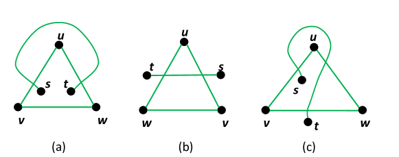
Figure 1: (a) An almost-planar topological graph $G$; (b) a straight-line drawing of $G$ that preserves its embedding on the sphere but not on the plane; (c) An almost-planar topological graph for which an embedding preserving straight-line drawing does not exist.

It is important to remark that by “preserving the embedding” we mean that the straight-line drawing must preserve the cyclic order of the edges around each vertex and around each crossing. In other words, we want to preserve a given embedding on the sphere. Note that the problem is different if, in addition to preserving the cyclic order of the edges around the vertices and the crossings, we also want the preservation of a given external boundary; in other words the problem is different if we want to maintain a given embedding on the plane instead of on the sphere. For example, consider the graph of Fig. 1(a). If we regard this as a topological graph on the sphere, then it has an embedding preserving straight-line drawing, as shown in Fig. 1(b). However, the drawing in Fig. 1(a) has a different external face to Fig. 1(b). It is easy to show that there is no straight-line drawing with the same external face as in Fig. 1(a). For a contrast, Fig. 1(c) shows a topological graph $G$ that does not have a straight-line drawing that preserves the embedding on the sphere.

In this paper we mostly focus on spherical topologies but, as a byproduct, we obtain a result for topologies on the plane that may be of independent interest. Namely, the main results of this paper are as follows.

• We characterize those almost-planar topological graphs that admit a straight-line drawing that preserves a given embedding on the sphere. The characterization gives rise to a linear-time testing algorithm.

• We characterize those almost-planar topological graphs that admit a straight-line drawing that preserves a given embedding on the plane.

• We present a drawing algorithm that constructs straight-line drawings when such drawings exist. This drawing algorithm runs in linear time; however, the model of computation used is the real RAM, and the drawings that are produced have exponentially bad resolution. We show that, in the worst case, the exponentially bad resolution is inevitable.

Our results also contribute to the rapidly increasing literature about topological graphs that are “nearly” plane, in some sense. An interesting example is the class of 1-plane graphs, that is, topological graphs with at most one crossing per edge. Thomassen [12] gives a “Fáry-type theorem” for 1-plane graphs, that is, a characterization of 1-plane topological graphs that admit a straight-line drawing. Hong et al. [8] present a linear-time algorithm that constructs a straight-line 1-planar drawing of 1-plane graph, if it exists. More generally, Nagamochi [11] investigates straight-line drawability of a wide class of topological non-planar topological graphs. He presentes Fáry-type theorems as well as polynomial-time testing and drawing algorithms. This paper considers graphs that are “nearly plane” in the sense that deletion of a single edge yields a planar graph. Such graphs are variously called “1-skew graphs” or “almost-planar” graphs in the literature. Our characterization can be regarded as a Fáry-type theorem for almost-planar graphs.

The rest of the paper is organized as follows. Section 2 gives notation and terminology. The characterization of almost-planar topological graphs on the sphere that admit an embedding preserving straight-line drawing is given in Section 3. The extension of this characterization to topological graphs on the plane and the exponential area lower bound are described in Section 4. Open problems can be found in Section 5.

2 Preliminaries

A topological graph $G=(V,E)$ is a representation of a simple graph on a given surface, where each vertex is represented by a point and each edge is represented by a simple Jordan arc between the points representing its endpoints. If the given surface is the sphere, then we say that $G$ is an $\mathbb{S}^{2}$-topological graph; if the given surface is the plane, then we say that $G$ is an $\mathbb{R}^{2}$-topological graph. Two edges of a topological graph cross if they have a point in common, other than their endpoints. The point in common is called a crossing. We assume that a topological graph satisfies the following non-degeneracy conditions: (i) an edge does not contain a vertex other than its endpoints; (ii) edges must not meet tangentially; (iii) no three edges share a crossing; and (iv) an edge does not cross an incident edge.

An $\mathbb{S}^{2}$-embedding of a graph is an equivalence class of $\mathbb{S}^{2}$-topological graphs under homeomorphisms of the sphere. An $\mathbb{S}^{2}$-topological graph has no unbounded face; in fact an $\mathbb{S}^{2}$-embedding is uniquely determined merely by the clockwise order of edges around each vertex and each edge crossing. An $\mathbb{R}^{2}$-embedding of a graph is an equivalence class of $\mathbb{R}^{2}$-topological graphs under homeomorphisms of the plane. Note that one face of an $\mathbb{R}^{2}$-topological graph in the plane is unbounded; this is the external face.

The concepts of $\mathbb{R}^{2}$-embedding and $\mathbb{S}^{2}$-embedding are very closely related. Each $\mathbb{S}^{2}$-topological graph gives rise to a representation of the same graph on the plane, by a stereographic projection about an interior point of a chosen face. This chosen face becomes the external face of the $\mathbb{R}^{2}$-topological graph. Thus we can regard an $\mathbb{R}^{2}$-embedding to be an $\mathbb{S}^{2}$-embedding in which one specific face is chosen to be the external face. Further, each $\mathbb{R}^{2}$-topological graph gives rise to a representation of the same graph on the sphere, by a simple projection.

A topological graph (either on the plane or on the sphere) is planar if no two edges cross. A topological graph is almost-planar if it has an edge $(s,t)$ whose removal makes it planar. An almost-planar $\mathbb{R}^{2}$-embedding ($\mathbb{S}^{2}$-embedding) of a graph is an equivalence class of almost-planar $\mathbb{R}^{2}$-topological graphs ($\mathbb{S}^{2}$-topological graphs) under homeomorphisms of the plane (sphere).

Throughout this paper, $G=(V,E)$ denotes an almost-planar topological graph ($\mathbb{S}^{2}$ or $\mathbb{R}^{2}$) and $(s,t)$ denotes an edge of $G$ whose deletion makes $G$ planar. The embedding obtained by deleting the edge $(s,t)$ is denoted by $\hat{G}$. More generally, we use the convention that the notation $\hat{X}$ normally denotes $X$ without the edge $(s,t)$.

Let $G$ be an $\mathbb{S}^{2}$-topological graph and let $G^{\prime}$ be an $\mathbb{R}^{2}$-topological graph with the same underlying simple graph. We say that $G^{\prime}$ preserves the $\mathbb{S}^{2}$-embedding of $G$ if for each vertex and for each crossing they have the same cyclic order of incident edges. Further, let $G$ be an $\mathbb{R}^{2}$-topological graph and let $G^{\prime}$ be an $\mathbb{R}^{2}$-topological graph with the same underlying simple graph. We say that $G^{\prime}$ preserves the $\mathbb{R}^{2}$-embedding of $G$ if for each vertex and for each crossing they have the same cyclic order of incident edges and the same external face. A straight-line drawing of a graph is an $\mathbb{R}^{2}$-topological graph whose edges are represented by straight-line segments.

3 Straight-line drawability of an almost-planar $\mathbb{S}^{2}$-embedding

In this section we state our main theorem. Let $G$ be a topological graph with a given almost-planar $\mathbb{S}^{2}$-embedding. Suppose that $\alpha$ is a crossing between edges $(s,t)$ and $(u,v)$ in $G$. If the clockwise order of vertices around $\alpha$ is $\langle s,u,t,v\rangle$, then $u$ is a left vertex and $v$ is a right vertex (with respect to the ordered pair $(s,t)$ and the crossing $\alpha$). We say that a vertex of $G$ is inconsistent if it is both left and right, and consistent otherwise. For example, vertex $v$ in Fig. 1(c) is inconsistent: it is a left vertex with respect the first crossing along $(s,t)$, and it is a right vertex with respect to the final crossing along $(s,t)$.

Theorem 3.1

An almost-planar $\mathbb{S}^{2}$-topological graph $G$ with $n$ vertices admits an $\mathbb{S}^{2}$-embedding preserving straight-line drawing if and only if every vertex of $G$ is consistent. This condition can be tested in $O(n)$ time.

The necessity of every vertex being consistent is straightforward. The proof of sufficiency involves many technicalities and it occupies most of the remainder of this paper. Namely, we prove the sufficiency of the condition in Theorem 3.1 by the following steps.

Augmentation:

We show that we can add edges to an almost-planar $\mathbb{S}^{2}$-topological graph to form a maximal almost-planar graph, without changing the property that every vertex is consistent. Let $G^{\prime}$ be the augmented $\mathbb{S}^{2}$-topological graph (subsection 3.1).

Choice of an external face:

We find a face $f_{o}$ of $G^{\prime}$ such that if the $\mathbb{S}^{2}$-embedding of $G^{\prime}$ is projected on the plane with $f_{0}$ as the external face, $G^{\prime}$ satisfies an additional property that we call face consistency (subsection 3.2).

Split the augmented graph:

After having projected $G^{\prime}$ on the plane with $f_{o}$ as the external face, we split the $\mathbb{R}^{2}$-embedding of $G^{\prime}$ into the “inner graph” and the “outer graph”. The inner graph and outer graph share a cycle called the “separating cycle” (subsection 3.3).

Straight-line drawing computation:

We draw the outer graph leaving a convex shaped “hole” for the inner graph; the boundary of this hole is the separating cycle. Then we draw the “inner graph”, whose external face is the separating cycle, such that it fits exactly into the convex shaped “hole” (subsections 3.4 and 3.5).

Before presenting more details of the proof of sufficiency, we observe that the condition stated in Theorem 3.1 can be tested in linear time. By regarding crossing points as dummy vertices, we can apply the usual data structures for plane graphs to almost-planar graphs (see [5], for example). A simple traversal of the crossing points along the edge $(s,t)$ can be used to compute the left and the right vertices. Since the number of crossing points in an almost-planar graph is linear, these data structures can be applied without asymptotically increasing total time complexity.

3.1 Augmentation

Let $G$ be an $\mathbb{S}^{2}$-topological graph. An $\mathbb{S}^{2}$-embedding preserving augmentation of $G$ is an $\mathbb{S}^{2}$-topological graph $G^{\prime}$ obtained by adding edges (and no vertices) to $G$ such that for each vertex (for each crossing) of $G^{\prime}$, the cyclic order of the edges of $G^{\prime}\cap G$ around the vertex (around the crossing) is the same in $G^{\prime}$ and in $G$. An almost-planar topological graph is maximal if the addition of any edge would result in a topological graph that is not almost planar. The following lemma describes a technique to compute an $\mathbb{S}^{2}$-embedding preserving augmentation of an almost-planar $\mathbb{S}^{2}$-topological graph that gives rise to a maximal almost-planar graph.

Lemma 1

Let $G$ be an almost-planar $\mathbb{S}^{2}$-topological graph with $n$ vertices. If $G$ satisfies the vertex consistency condition, then there exists a maximal almost-planar $\mathbb{S}^{2}$-embedding preserving augmentation $G^{\prime}$ of $G$ such that $G^{\prime}$ satisfies the vertex consistency condition. Also, such augmentation can be computed in $O(n)$ time.

Proof

We add as many edges as possible to $G$ without introducing any new crossing. Let $\tilde{G}$ be the resulting $\mathbb{S}^{2}$-topological graph. Since $\tilde{G}$ was constructed from $G$ without adding any edge crossings, $\tilde{G}$ is an almost-planar $\mathbb{S}^{2}$-topological graph and it has the same set of left vertices and the same set of right vertices as $G$. If $\tilde{G}-(s,t)$ is a maximal planar graph we are done. So assume $\tilde{G}$ otherwise, which implies that there is at least one face of $\tilde{G}-(s,t)$ that has size larger than three. Fig. 2(a) shows an example of an almost-planar topological graph $G$ and Fig. 2(b) shows an example of a (non-maximal) graph $\tilde{G}$.

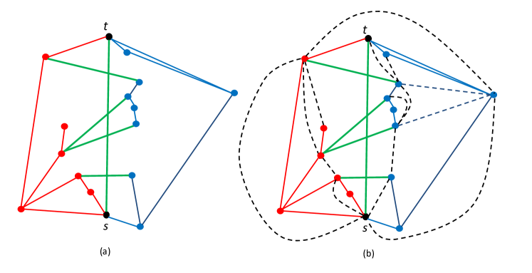
Figure 2: (a) A non maximal almost-planar graph $G$. (b) Graph $\tilde{G}$ obtained by adding the dotted edges.

Denote the edges of $G$ that cross $(s,t)$ by $e_{0},e_{1},\dots,e_{p-1}$, ordered from $s$ to $t$ by their crossings along $(s,t)$. Suppose that $e_{i}=(\ell_{i},r_{i})$ for $0\leq i<p$, where $\ell_{i}$ is a left vertex and $r_{i}$ is a right vertex. By construction, $\tilde{G}$ is such that $\ell_{0}$ is adjacent to $s$. If not, we could have added edge $(\ell_{0},s)$ to $\tilde{G}$ by closely following the edge $e_{0}$ from $\ell_{0}$ to the crossing with $(s,t)$ and then by closely following the edge $(s,t)$ from this crossing down to $s$, till we encounter $s$, without introducing any new edge crossings. With similar reasoning, it is immediate to see that, in $\tilde{G}$, vertex $r_{0}$ is adjacent to $s$ and that $\ell_{p-1}$ and $r_{p-1}$ are both adjacent to $t$. Also, any two consecutive edges $e_{i}=(\ell_{i},r_{i})$ and $e_{i+1}=(\ell_{i+1},r_{i+1})$ either have an endvertex in common or graph $\tilde{G}$ contains edges $(\ell_{i},\ell_{i+1})$ and $(r_{i},r_{i+1})$ (or we could have added them without crossing edge $(s,t)$ by closely following $e_{i+1}$ from an endvertex to its crossing with $(s,t)$, then closely following $(s,t)$ from this crossing down to the crossing between $(s,t)$ and $e_{i}$, and finally closely following $e_{i}$ to its endvertex).

Let $C_{0}$ be the cycle of $\tilde{G}$ induced by vertices $s$, $\ell_{0}$, and $r_{0}$; let $C_{p-1}$ be the cycle induced by vertices $t$, $\ell_{p-1}$, and $r_{p-1}$; for $1\leq i<p-1$, let $C_{i}$ be the cycle of $\tilde{G}$ induced by vertices $\ell_{i}$, $r_{i}$, $\ell_{i+1}$, and $r_{i+1}$. Note that $C_{0}$ and $C_{p-1}$ are 3-cycles, while $C_{i}$ may be either a 3-cycle or a 4-cycle depending on whether edges $e_{i}$ and $e_{i+1}$ have an endvertex in common or not. See, for example, Fig. 2(b) where some of such cycles are 3-cycles and some other such cycles are 4-cycles. For each cycle $C_{0},C_{1},\dots,C_{p-1}$ we define the interior of the cycle as the region that contains a portion of the edge $(s,t)$.

Consider $C_{0}$ first and the edge $(\ell_{0},s)$. Since $\tilde{G}$ is constructed by adding as many edges as possible to $G$ that do not cross edge $(s,t)$, we have that $(\ell_{0},s)$ is an edge of some triangular face of $\tilde{G}$. Let $v$ be the vertex of $f$ different from $\ell_{0}$ and $s$. Either $v$ is in the interior of $C_{0}$ or not. Similarly, let $w$ be the vertex opposite to $(r_{0},s)$ in some triangular face of $\tilde{G}$; either $w$ is in the interior of $C_{0}$ or not. We distinguish between three cases (see Fig. 3): One of $v$ and $w$ is in the interior of $C_{0}$, both $v$ and $w$ are in the interior of $C_{0}$, and none of $v$ and $w$ is in the interior of $C_{0}$. Consider the first case and assume, w.l.o.g., that $v$ is in the interior of $C_{0}$ while $w$ is not. Note that $v$ was neither a left vertex nor a right vertex of $G$; it cannot be a left vertex because there would be an edge crossing $(s,t)$ that is encountered before $e_{0}$ when going from $s$ to $t$. It cannot be a right vertex, because the edge incident to $v$ and crossing $(s,t)$ should also intersect edge $(s,\ell_{0})$, which is impossible.

We add an edge connecting $v$ with $r_{0}$ as described by the dotted edge in Fig. 3(a): Start at $v$ and closely follow edge $(v,\ell_{0})$, then closely follow edge $(\ell_{0},r_{0})$ till $r_{0}$ is reached. Note that $v$ has become a left vertex and that the vertex consistency condition holds for all other vertices. Consider now the case that both $v$ and $w$ are in the interior of $C_{0}$ (see Fig. 3(b)). Also in this case, both $v$ and $w$ are neither left nor right vertices of $G$. We add edge $(v,r_{0})$ as in the previous case; then we add edge $(v,w)$ by starting at $w$, closely following edge $(w,s)$, then closely following edge $(s,v)$, and finally ending at vertex $v$. In this case $v$ has become a left vertex, $w$ is a right vertex, and the vertex consistency condition holds for all other vertices. Finally, if neither $v$ nor $w$ is in the interior of $C_{0}$, no edge crossing $(s,t)$ is added in its interior and the vertex condition consistency is trivially maintained.

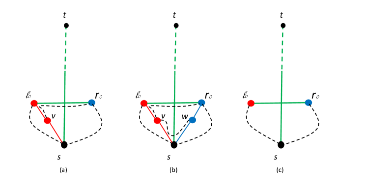
Figure 3: (a) The interior of $C_{0}$ contains a vertex $v$. (b) The interior of $C_{0}$ contains two vertices $v$ and $w$. (c) The interior of $C_{0}$ does not contain vertices.

For each cycle $C_{i}$ ($1\leq i<p-1$) such that $C_{i}$ is not a 3-cycle we add an edge in its interior that only crosses edge $(s,t)$ as follows: Starting at vertex $\ell_{i}$, we closely follow edge $e_{i}$ until the crossing between $e_{i}$ and $(s,t)$ is encountered; next, we closely follow edge $(s,t)$ upward to its crossing with $e_{i+1}$; finally, we closely follow edge $e_{i+1}$ until we reach vertex $r_{i+1}$; see Fig. 4(a) for an illustration of this step. Note that since edge $(\ell_{i},r_{i+1})$ is added in the interior of $C_{i}$, we have that $\ell_{i}$ remains a left vertex and $r_{i+1}$ remains a right vertex after such an edge insertion. Consider now the 3-cycle with vertices $\ell_{i}$, $r_{i+1}$, and $\ell_{i+1}$ and the the 3-cycle with vertices $r_{i}$, $r_{i+1}$, and $\ell{i}$. As with the case of $C_{0}$, each such 3-cycle may have a vertex $v$ in its interior such that $v$ is neither a left vertex nor a right vertex of $G$. We add an edge incident to $v$ and crossing edge $(s,t)$ and no other edges of the graph with the same technique described for $C_{0}$; see Fig. 4(b) for an example of this edge addition.

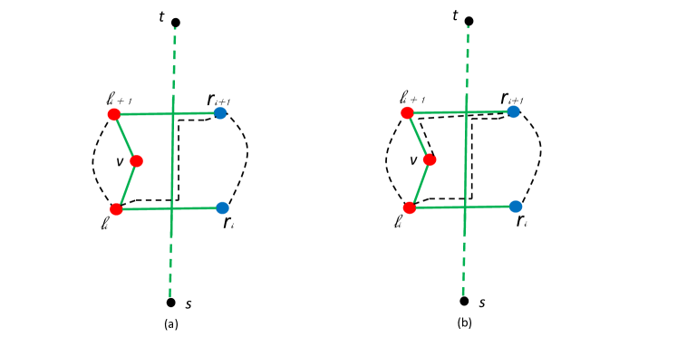
Figure 4: (a) $C_{i}$ is a 4-cycle and the dotted edge splits it into two 3-cycles. (b) A dotted edge crossing $(s,t)$ and incident to a vertex $v$ is added; $v$ becomes a left vertex.

Finally, edges are added inside cycle $C_{p-1}$ with the same approach described for $C_{0}$.

Let $G^{\prime}$ be the resulting $\mathbb{S}^{2}$-topological graph. The proof is concluded by observing that: (i) $G^{\prime}$ is an almost-planar $\mathbb{S}^{2}$-embedding preserving augmentation $G$ and it has $3n-5$ edges, and (ii) $G^{\prime}$ can be constructed in linear time by a simple traversal of the faces in a standard data structure for planar graphs adapted to represent almost-planar graphs (see [5], for example). ∎

It would be tempting to suggest that a maximal almost-planar topological graph consists of a maximal planar graph plus an edge. This is not quite true; see Fig 5.

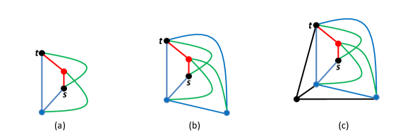
Figure 5: Maximal almost-planar graphs with $3n-6$ edges.

However, we can prove that a maximal almost-planar topological graph “almost” consists of a maximal planar graph plus an edge. To this aim, we need a preliminary result.

Lemma 2

Suppose that $f$ is a face of the topological subgraph $\hat{G}$ of a maximal almost-planar topological graph $G$ formed by deleting the edge $(s,t)$.

1. The subgraph $G_{f}$ of $G$ induced by the vertices of $f$ is a clique in $G$.

2. The subgraph $\hat{G}_{f}$ of $\hat{G}$ induced by the vertices of $f$ is an outerplane graph.

Proof

Since $G$ is a maximal almost-planar graph, if $u$ and $v$ are vertices of $f$ then either $(u,v)$ is already an edge of $\hat{G}$ or $u$ and $v$ coincide with $s$ and $t$, respectively. In either case, $(u,v)$ is an edge of $G$. This proves (1). Further, since $f$ is a face of $\hat{G}$, every edge of this clique of $G$ induced by $f$ lies outside or on the boundary of $f$. This proves (2). ∎

We are now ready to prove the following.

Lemma 3

If $G$ is a maximal almost-planar topological graph, then either $\hat{G}$ is a maximal planar graph (that is, every face of $\hat{G}$ has size 3); or every face of $\hat{G}$ has size 3, except exactly one face $f_{4}$ which has the following properties: (i)$f_{4}$ has size 4; (ii)$f_{4}$ induces a clique in $G$; and (iii) both $s$ and $t$ are on $f_{4}$.

Proof

Let $G$ be a maximal almost-planar topological graph. Let $m$ denote the number of edges of $G$. Since $\hat{G}$ is planar, $m\leq 3n-5$. Suppose that $\hat{G}$ is not a maximal planar graph, that is, $m\leq 3n-6$.

First consider the case that $m\leq 3n-7$, that is, $\hat{G}$ has at most $3n-8$ edges. Simple counting shows that $\hat{G}$ either contains a face with more than four vertices or it has at least two faces each having four vertices.

Suppose first that $\hat{G}$ has a face $f$ with $k\geq 5$ vertices. From Lemma 2(1), $\hat{G}_{f}$ has at least $\frac{k(k-1)}{2}-1$ edges. From Lemma 2(2), $\hat{G}_{f}$ has at most $2k-2$ edges. However, $\frac{k(k-1)}{2}-1>2k-2$ if $k>4$; thus $\hat{G}$ cannot have a face with at least five vertices.

Suppose now that $\hat{G}$ has two faces $f_{1}$ and $f_{2}$ each having four vertices. From Lemma 2, $G_{f_{i}}$ has 6 edges and $\hat{G}_{f_{i}}$ has 5 edges, for both $i=1$ and $i=2$. Thus $s$ and $t$ must be vertices of both $f_{1}$ and $f_{2}$. Hence, $f_{1}$ and $f_{2}$ are as in Fig. 6; consider vertices $u$ and $v$ in the figure: they must be adjacent in $\hat{G}$, but edge $(u,v)$ would either split face $f_{1}$ or introduce a crossing. It follows that $\hat{G}$ cannot have two faces with four vertices.

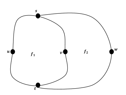
Figure 6: If $\hat{G}$ has two faces each having four vertices, then $G$ is not a maximal almost-planar graph.

Finally consider the case that $m=3n-6$. Counting reveals that every face of $\hat{G}$ has size 3, except exactly one face $f_{4}$ has size 4. The other properties of $f_{4}$ follow from Lemma 2.

3.2 Choice of an external face

The augmentation step results in a maximal almost-planar $\mathbb{S}^{2}$-topological graph $G^{\prime}$ in which every vertex is consistent. Next, we want to identify a face $f_{o}$ of $G^{\prime}$ such that if we choose $f_{0}$ to be the external face, then $G^{\prime}$ becomes an $\mathbb{R}^{2}$-topological graph that has an embedding preserving straight-line drawing in the plane. To identify such a face, we need some further terminology.

Let $G$ be an almost-planar topological graph. Let $\hat{G}$ denote $G-(s,t)$. We denote the set of left (resp. right) vertices of $G$ by $V_{L}$ (resp. $V_{R}$). We denote the subgraph of $\hat{G}$ induced by $V_{L}\cup\{s,t\}$ (resp. $V_{R}\cup\{s,t\}$) by $\hat{G}_{L}$ (resp. $\hat{G}_{R}$). The union of $\hat{G}_{L}$ and $\hat{G}_{R}$ is $\hat{G}_{LR}$, and $G_{LR}$ denotes the topological subgraph of $G$ formed from $\hat{G}_{LR}$ by adding the edge $(s,t)$. Note that $G_{LR}$ and $\hat{G}_{LR}$ are not necessarily induced subgraphs of $\hat{G}$. A face of $G_{LR}$ is inconsistent if it contains a left vertex and a right vertex, and consistent otherwise. In fact we can prove that vertex consistency implies that $G_{LR}$ has exactly one inconsistent face. But first we prove some simple results about $G_{LR}$ .

Lemma 4

Let $G$ be an $\mathbb{S}^{2}$-topological graph in which every vertex is consistent and let $C$ be a simple cycle in $G_{LR}$ with at least one left vertex and at least one right vertex. Then $C$ contains $s$ and $t$.

Proof

Note that $G_{LR}$ has no edge that joins a left vertex to a right vertex. Thus all paths from a left vertex to a right vertex pass through either $s$ or $t$, and thus $C$ contains both $s$ and $t$. ∎

Lemma 5

If $G$ is an almost-planar topological graph then $\hat{G}_{LR}$ is outerplanar.

Proof

The edge $(s,t)$ passes through a face $f$ of $\hat{G}_{LR}$, and $s$ and $t$ are on that face. Further, every left vertex $\ell$ is on $f$ because, in $G$, there is an edge incident to $\ell$ that crosses $(s,t)$. Similarly every right vertex is on $f$. ∎

We first prove that $G_{LR}$ cannot have two inconsistent faces and then show that $G_{LR}$ always has one inconsistent face.

Lemma 6

Let $G$ be an almost-planar $\mathbb{S}^{2}$-topological graph in which every vertex is consistent. Then $G_{LR}$ has at most one inconsistent face.

Proof

Suppose that $G_{LR}$ had two inconsistent faces, say $f_{0}$ and $f_{1}$. Make a projection on the plane so that $f_{0}$ becomes the external face of an $\mathbb{R}^{2}$-embedding of $G_{LR}$. The boundary of $f_{0}$ contains a simple cycle with at least one left vertex and at least one right vertex; by Lemma 4, vertices $s$ and $t$ are vertices along the boundary of $f_{0}$. Also, there exists a simple path on the boundary of $f_{0}$ that starts at $s$, ends at $t$, and is such that any other vertex of the path is a left vertex; we call such a path the left path of $f_{0}$ and denote it as $\Pi_{L}$. Similarly, the right path $\Pi_{R}$ of $f_{0}$ is the simple path along the boundary of $f_{0}$ whose endvertices are $s$ and $t$ and such that any internal vertex is a right vertex of $f_{0}$. Observe that edge $(s,t)$ is inside face $f_{0}$ since $f_{0}$ is chosen as the external face in the $\mathbb{R}^{2}$-embedding of $G$.

The left cycle of $G$ is the simple cycle consisting of $\Pi_{L}\cup(s,t)$; the right cycle of $G$ is the simple cycle consisting of $\Pi_{R}\cup(s,t)$. Every vertex that does not belong to $f_{0}$ is either strictly inside the left cycle or strictly inside the right cycle. Note that any vertex $v$ of $G_{LR}$ inside the left cycle must be a left vertex. Namely, $v$ is the endvertex of an edge $e$ that crosses edge $(s,t)$. Since $G$ is almost-planar, edge $e$ cannot cross any other edge of $G$ except $(s,t)$. Therefore edge $e$ crosses $(s,t)$ without intersecting the boundary of $f_{0}$, which implies that $v$ is a left vertex. Similarly, every vertex of $G_{LR}$ inside the right cycle is a right vertex.

Consider now face $f_{1}$; $f_{1}$ must be entirely inside either the left cycle or entirely inside the right cycle. However, $f_{1}$ is inconsistent and therefore it has both left vertices and right vertices, which contradicts the fact that all vertices inside the left cycle are left vertices and all vertices inside the right cycle are right vertices.∎

Lemma 7

Suppose that $G$ is a maximal almost-planar $\mathbb{S}^{2}$-topological graph in which every vertex is consistent. Then $G_{LR}$ has at least one inconsistent face, and this face is a simple cycle.

Proof

Let $q_{L}$ be a shortest path in $\hat{G}_{L}$ from $s$ to $t$, and let $q_{R}$ be a shortest path in $\hat{G}_{R}$ from $t$ to $s$. The existence of such paths is guaranteed by maximality. Further, since $(s,t)$ is not in either $\hat{G}_{L}$ or $\hat{G}_{R}$, $q_{L}$ contains at least one left vertex and $q_{R}$ contains at least one right vertex. From Lemma 5, the cycle $C$ formed by concatenating $q_{L}$ and $q_{R}$ forms a face $f$ of $\hat{G}_{LR}$.

If $f$ is also a face of $G_{LR}$, then the Lemma follows. Otherwise $(s,t)$ must “split” $f$ in $\hat{G}_{LR}$. In this case, every left and every right vertex must lie on $f$; it follows that $\hat{G}_{LR}$ is exactly $f$. The Lemma follows, since $(s,t)$ can be on only one side of the cycle $C$. ∎

Lemma 6 and Lemma 7 imply the following.

Lemma 8

Let $G$ be an $\mathbb{S}^{2}$-topological graph in which every vertex is consistent. Then $G_{LR}$ has exactly one inconsistent face.

We now proceed as follows. Let $G$ be an $\mathbb{S}^{2}$-topological graph in which every vertex is consistent and let $G^{\prime}$ be a maximal almost-planar $\mathbb{S}^{2}$-embedding preserving augmentation of $G$ constructed by using Lemma 1. We project $G$ on the plane such that the only inconsistent face of $G_{LR}$ is its external face. The following lemma is a consequence of the discussion above and of Lemma 8.

Lemma 9

Let $G$ be a maximal almost-planar $\mathbb{S}^{2}$-topological graph in which every vertex is consistent. There exists an $\mathbb{R}^{2}$-topological graph $G^{\prime}$ that preserves the $\mathbb{S}^{2}$-embedding of $G$ and such that: (i) every internal face of $\hat{G^{\prime}}$ consists of three vertices (i.e. it is a triangle); (ii) every internal face of $G^{\prime}_{LR}$ is consistent.

Examples of an almost-planar $\mathbb{R}^{2}$-topological graph $G$ and of its subgraphs $\hat{G_{L}}$, $\hat{G_{R}}$, and $G_{LR}$ are given in Fig. 7 and Fig. 8.

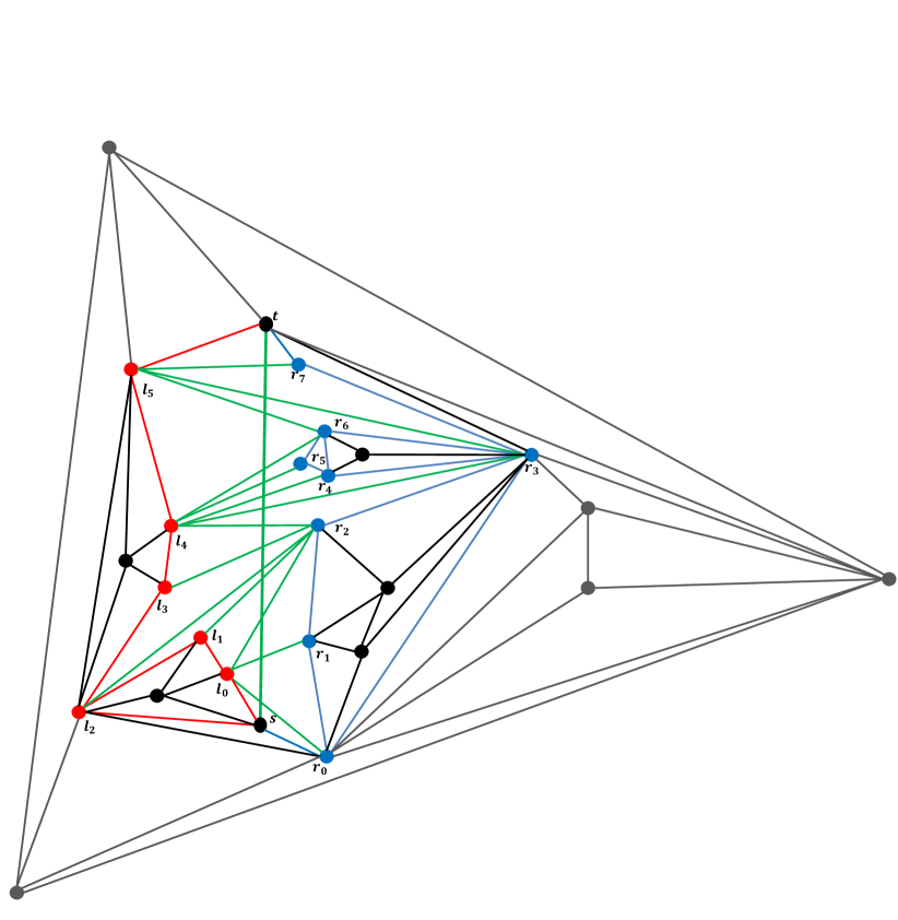
Figure 7: An almost-planar $\mathbb{R}^{2}$-topological graph $G$. Left vertices are red and labelled $l_{i}$, $i=0,\ldots,5$; right vertices are blue and labelled $r_{i}$, $i=0,\ldots,7$.

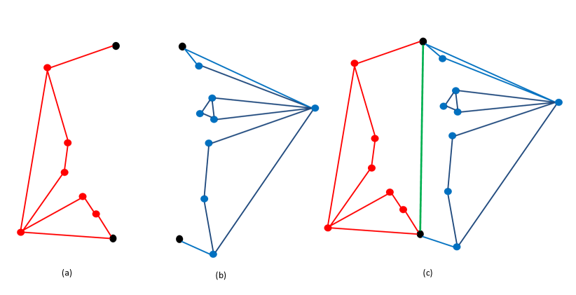
Figure 8: Subgraphs of the graph $G$ in Fig. 7: (a) $\hat{G}_{L}$, (b) $\hat{G}_{R}$, (c) $G_{LR}$.

3.3 Splitting the augmented graph

For the remainder of Section 3, we assume that $G$ is a maximal almost-planar $\mathbb{R}^{2}$-topological graph; that is, that the augmentation and choice of an outer face have been done. Next we divide $G$ into the “inner graph” and the “outer graph”.

Denote the induced subgraph of $\hat{G}$ on the vertex set $V_{L}\cup V_{R}\cup\{s,t\}$ by $\hat{G}^{+}_{LR}$. Note that $\hat{G}_{LR}$ is a subgraph of $\hat{G}^{+}_{LR}$, but these graphs may not be the same; in particular, $\hat{G}^{+}_{LR}$ may have edges with a left endpoint and a right endpoint that do not cross $(s,t)$; such an edge is called a cap edge. Although $\hat{G}$ is internally triangulated by Lemma 9, $\hat{G}^{+}_{LR}$ may have non-triangular inner faces. Fig. 9(a) shows $\hat{G}^{+}_{LR}$, where $G$ is the graph in Fig. 7. The non-triangular inner faces in Fig. 9(a) arise, for example, from cycles of left vertices in Fig. 7 that have vertices that are neither left nor right in their interior. Examples are in Fig. 9(a).

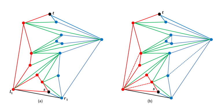
Figure 9: (a) $\hat{G}^{+}_{LR}$, where $G$ is in Fig. 7; here $(\ell_{1},r_{1})$ is a cap edge. (b) The inner graph $\hat{G}_{in}$.

To following lemma states that the external face of $\hat{G}^{+}_{LR}$ is a simple cycle. It can be proved with the same method as used in the proof of Lemma 7. We can show that the concatenation $C$ of the shortest paths $q_{L}$ and $q_{R}$ is the boundary of the external face of $\hat{G}_{LR}$; thus the external face of $\hat{G}_{LR}$ is a simple cycle. Since $\hat{G}^{+}_{LR}$ is an induced subgraph with the same vertex set as $\hat{G}_{LR}$, it follows that the external face of $\hat{G}^{+}_{LR}$ is a simple cycle.

Lemma 10

If $G$ is a maximal almost-planar $\mathbb{R}^{2}$-topological graph such that every internal face of $G_{LR}$ is consistent, then the external face of $\hat{G}^{+}_{LR}$ is a simple cycle.

We call the external face of $\hat{G}^{+}_{LR}$ the separating cycle of the graph $G$. The topological subgraph consisting of the separating cycle as well as all vertices and edges that lie outside the separating cycle is the outer graph $G_{out}$. Fig.10 is an example of outer graph.

Figure 10: The outer graph for the graph in Fig. 7(a).

The inner graph consists of $\hat{G}^{+}_{LR}$ with the addition of some dummy edges. Namely, for every face $f$ of $\hat{G}^{+}_{LR}$ that is not a triangle, we perform a fan triangulation; that is, we choose a vertex $u$ of $f$ with degree 2 in $f$, and add dummy edges incident with $u$ to triangulate $f$. The graph formed by fan triangulating every non-triangular internal face of $\hat{G}^{+}_{LR}$ is the inner graph $\hat{G}_{in}$.

Note that the vertices of $G$ that are neither left vertices nor right vertices and that are inside the separating cycle belong to neither the inner nor the outer graph. At the end of next section we show how to reinsert these vertices and their incident edges into the drawing.

3.4 Drawing the outer graph

Since $G$ is maximal almost-planar, by using Lemma 3 we can show that $G_{out}$ is triconnected as long as the separating cycle has no chord. But since $G_{in}$ contains the subgraph of $\hat{G}$ induced by the separating cycle, every chord on the separating cycle is in $G_{in}$ and not in $G_{out}$. Thus $G_{out}$ is triconnected. We use the linear-time convex drawing algorithm of Chiba et al. [4] to draw $G_{out}$ such that every face in the drawing is a convex polygon. This drawing of the outer graph has a convex polygonal drawing of the separating cycle, which we shall call the separating polygon. In the next section we show how to draw the inner graph such that its outside face (i.e. the separating cycle) is the separating polygon.

3.5 Drawing the inner graph

The overall approach for drawing the inner graph is described as follows. For each edge $e$ of the separating cycle, we define a “side graph” $S_{e}$; intuitively, $S_{e}$ consists on vertices and edges that are “close” to $e$. There may be two special side graphs, that contain cap edges (that is, edges that join a left vertex and a right vertex but do not cross $(s,t)$); these side graphs are “cap graphs”. Each side graph has a block-cutvertex tree $T_{e}$. We root $T_{e}$ at the block (biconnected component) that contains the edge $e$. The algorithm first draws the root block for each side graph, then proceeds from the root to the leaves of these trees, drawing the blocks one by one. Cap graphs are drawn with a different algorithm from that used for other side graphs.

Each non-root block $B$ in $T_{e}$ with parent cutvertex $c$ is associated with circular arc $\gamma(B)$, and two regions, called a “safe wedge” $\omega(B)$ and a “safe moon” $\mu(c)$; these are defined precisely below. We draw all the vertices of $B$ and its descendants in $\mu(c)$, with all vertices except $c$ lying on $\gamma(B)$ inside $\mu(c)\cap\omega(B)$. Every edge with exactly one endpoint in $B$ and its descendants lies inside $\omega(B)$.

First the root blocks are drawn, and then the algorithm proceeds by repeating the following steps until every vertex of every side graph is drawn. (1) Choose a “safe block” $B$ from the child blocks of drawn vertices; (2) Compute the “safe moon” $\mu(c)$, the “safe wedge” $\omega(B)$, and the circular arc $\gamma(B)$; (3) Draw each vertex of $B$ except $c$ on $\gamma(B)$.

Side graphs and cap graphs. To define “side graphs” and “cap graphs”, we need to first define a certain closed walk in the inner graph. Denote the edges that cross $(s,t)$ by $e_{0},e_{1},\dots,e_{p-1}$, ordered from $s$ to $t$ by their crossing points along $(s,t)$. Suppose that $e_{i}=(\ell_{i},r_{i})$ for $0\leq i\leq p-1$, where $\ell_{i}$ is a left vertex and $r_{i}$ is a right vertex. Note that cyclic list $(s,\ell_{0},\ell_{1},\ldots,\ell_{p-1},t,r_{p-1},\ldots,r_{1},r_{0})$ may contain repeated vertices.

Now let $W$ be the sublist of $(s,\ell_{0},\ell_{1},\ldots,\ell_{p-1},t,r_{p-1},\ldots,r_{1},r_{0})$ obtained by replacing each contiguous subsequence of the same vertex by a single occurrence of that vertex. Note that $W$ may contain repeated vertices, but these repeats are not contiguous. Namely, $W$ is a closed spanning walk of $\hat{G}_{LR}$. An example of this walk $W$ is in Fig. 11.

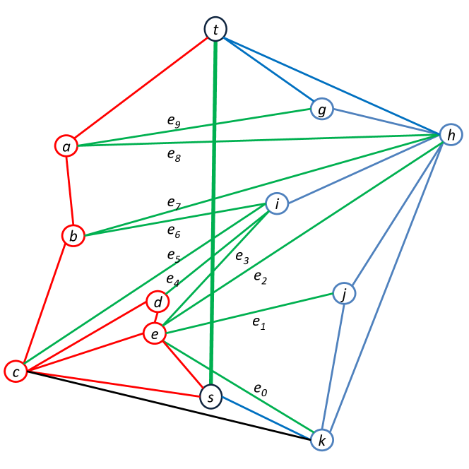
Figure 11: $W$ is the closed walk $(s,e,d,c,b,a,t,g,h,i,h,j,k)$.

Now let $e=(u,v)$ be an edge of the separating cycle, with $u$ before $v$ in clockwise order around the separating cycle. Note that both $u$ and $v$ are elements of the closed walk $W$. Suppose that the clockwise sequence of vertices in $W$ between $u$ and $v$ is $(u=u_{1},u_{2},\ldots,u_{k}=v)$. If $u$ occurs more than once in $W$, then we choose $u_{1}$ to be the first occurrence of $u$ in clockwise order after $s$; similarly choose $u_{k}$. The side graph $S_{e}$ is the induced subgraph of $G$ on $\{u_{1},u_{2},\ldots,u_{k}\}$.

If $S_{e}$ contains both left and right vertices then it is a cap graph. Note that a cap graph contains either $s$ or $t$; one can show that $s$ and $t$ are not in the same cap graph. Examples of side graphs, including cap graphs, are in Fig. 12.

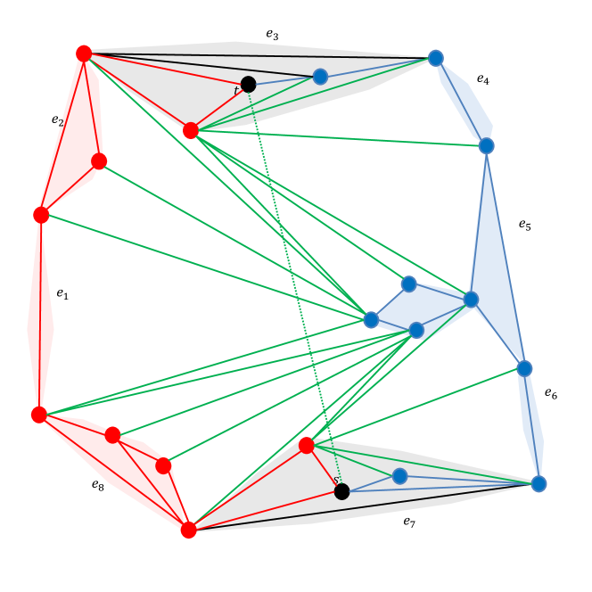
Figure 12: An inner graph with eight side graphs (shaded). This graph has two cap graphs $S_{e_{3}}$ and $S_{e_{7}}$.

Drawing the root blocks of side graphs. Next we show how to draw the root block $B^{*}_{e}$ of the side graph $S_{e}$. The edge $e$ is drawn as a side $\lambda_{e}$ of the separating polygon. We define a circular arc $\gamma(B^{*}_{e})$ through the endpoints of $\lambda_{e}$, with radius chosen such that the maximum distance from $\lambda_{e}$ to $\gamma(B^{*}_{e})$ is $\epsilon_{1}$. We will show how to choose $\epsilon_{1}$ later; for the moment, we assume that $\epsilon_{1}$ is very small in comparison to the length of the smallest edge of the separating polygon. The convex region bounded by $\lambda_{e}$ and $\gamma(B^{*}_{e})$ is called the pillow of $e$.

Suppose that $B^{*}_{e}$ of $S_{e}$ has $a+1$ vertices, which occur in clockwise order on the closed walk $W$ as $w_{0},w_{1},\ldots,w_{a}$. Since $B^{*}_{e}$ is biconnected, this sequence is a Hamilton path of $S_{e}$. We compute $a+1$ equally spaced points $\alpha(w_{0}),\alpha(w_{1}),\ldots,\alpha(w_{a})$ on $\lambda_{e}$ as in Fig. 13(a). Let $\zeta(w_{i})$ denote the line through $\alpha(w_{i})$ orthogonal to $\lambda_{e}$, as in Fig. 13(a).

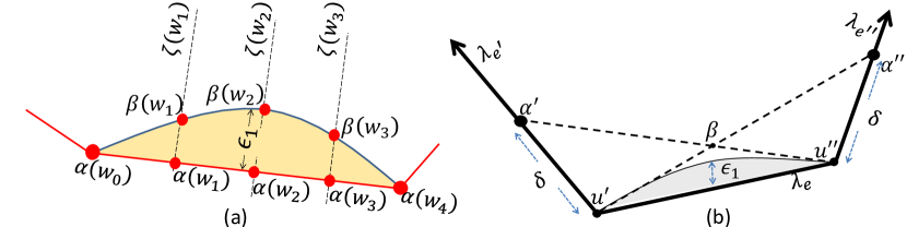
Figure 13: (a) A pillow. (b) Defining $\epsilon_{1}$.

If $S_{e}$ is not a cap graph, then we simply place vertex $w_{i}$ in $B^{*}_{e}$ at the point $\beta(w_{i})$ where $\zeta(w_{i})$ intersects the circular arc $\gamma(B^{*}_{e})$ ($0\leq i\leq a$). Note that the edges of $S_{e}$ (which are chords on the Hamilton path $(w_{0},w_{1},\ldots,w_{a})$) lie within the pillow of $e$.

If $S_{e}$ is a cap graph, then we place vertex $w_{i}$ on the line $\zeta(w_{i})$, but not necessarily at $\beta(w_{i})$. First we define an acyclic directed graph as follows. We direct edges along the Hamilton path $(w_{0},w_{1},\ldots,w_{a})$ from $w_{0}$ to $w_{a}$, and direct other edges so that the result is a directed acyclic graph $\overrightarrow{B^{*}_{e}}$ with a source at $w_{0}$ and a sink at $w_{a}$. Note that $\overrightarrow{B^{*}_{e}}$ is a leveled planar graph with one vertex on each level [10]. One can use the algorithm in [6] to draw $\overrightarrow{B^{*}_{e}}$ so that there are no edge crossings, vertex $w_{i}$ lies on the line $\zeta(w_{i})$, and the external face is a given polygon. We choose the external face to be the convex hull of $\lambda_{e}$ and the points $\beta(w_{i})$, $0\leq i\leq a$. Note that the vertices $w_{0},w_{1},\ldots,w_{a}$ are in monotonic order in the direction of the edge $(w_{0},w_{k})$. The general picture after the drawing of the root blocks is illustrated in Fig. 14.

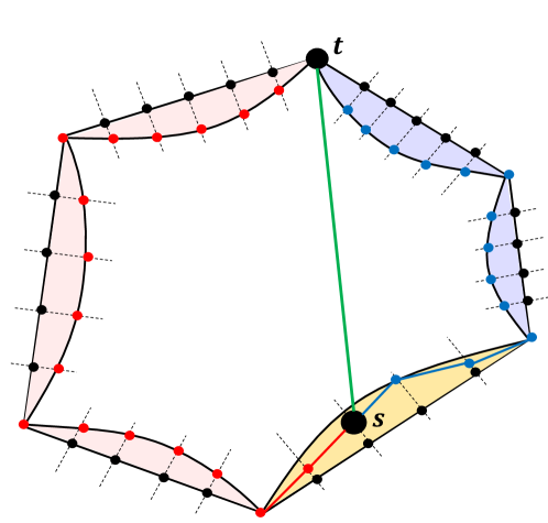
Figure 14: The general picture with pillows.

Next we show how to choose $\epsilon_{1}$. Let $\delta$ denote $d/n$, where $d$ is the minimum length of a side of the separating polygon, and $n$ is the number of vertices in the graph. Suppose that $\lambda_{e^{\prime}}$, $\lambda_{e}$, and $\lambda_{e^{\prime\prime}}$ are three consecutive sides of the separating polygon, as in Fig. 13(b); we show how to choose $\epsilon_{1}$ for the edge $e$. Suppose that the endpoints of $e$ are $u^{\prime}$ and $u^{\prime\prime}$, and $\alpha^{\prime}$ and $\alpha^{\prime\prime}$ are points on $\lambda_{e^{\prime}}$ and $\lambda_{e^{\prime\prime}}$ distant $\delta$ from $u^{\prime}$ and $u^{\prime\prime}$ respectively. Suppose that the line from $u^{\prime}$ to $\alpha^{\prime\prime}$ meets the line from $u^{\prime\prime}$ to $\alpha^{\prime}$ at $\beta$. Convexity ensures that $\beta$ is inside the separating polygon, and thus $(u^{\prime},\beta,u^{\prime\prime})$ forms a triangle inside the separating polygon. We choose $\epsilon_{1}$ so that the circular arc $\gamma(B^{*}_{e})$ through $u^{\prime}$ and $u^{\prime\prime}$ lies inside this triangle (meeting the triangle only on the line segment $\lambda_{e}$). The reason for this choice of $\epsilon_{1}$ is to ensure that all vertices in $B^{*}_{e}$ are so close to the side $\lambda_{e}$ of the separating polygon that it is impossible for an edge between different pillows to intersect with pillows other than those at its endpoints.

Safe blocks. To describe the algorithm for drawing the non-root blocks, we need some terminology. Suppose that $c$ is a cutvertex in the side graph $S_{e}$, and $B=(V_{B},E_{B})$ is a child block of $c$. Suppose that $c$ is a left vertex. In the clockwise order of edges in $G$ around $c$, there is an edge $e_{1}\not\in E_{B}$, followed by a number of edges in $E_{B}$, followed by an edge $e_{2}\not\in E_{B}$, as illustrated in Fig. 15(a). We say that $e_{1}$ and $e_{2}$ are the bounding edges of $B$. Note that a bounding edge either crosses $(s,t)$, or has $s$ or $t$ as an endpoint.

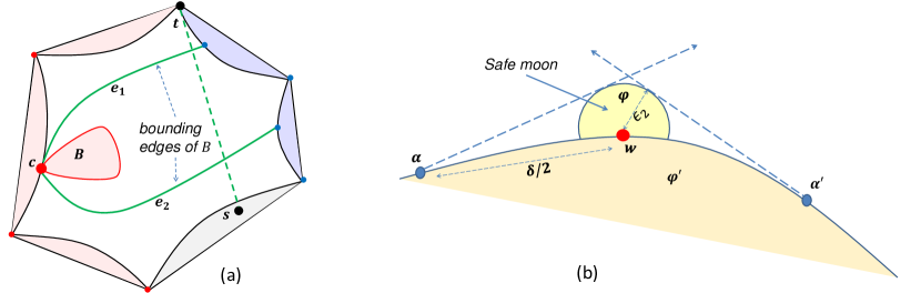
Figure 15: (a) Bounding edges of a block. (b)The safe moon $\mu(u)$ at $u$

.

At any stage of the drawing algorithm, a block may be safe or unsafe. A block $B$ is safe if the following properties hold: (i) The parent cutvertex $c$ (that is, the parent of $B$ in the block-cutvertex tree) has been drawn, and the other vertices in $B$ are not drawn; (ii) Suppose that the boundary edges of $B$ are $e_{1}=(c,u_{1})$ and $e_{2}=(c,u_{2})$; let $u^{\prime}_{1}$ and $u^{\prime}_{2}$ be the vertices which are the least already-drawn ancestors of $u_{1}$ and $u_{2}$ respectively in their respective block-cutvertex trees. Then we require that $u^{\prime}_{1}\not=u^{\prime}_{2}$.

Lemma 11

If there is an undrawn vertex, then there is a safe block.

Proof

Let $B$ be a block with parent cutvertex $c$ and boundary edges $(c,u_{1})$ and $(c,u_{2})$; let $u^{\prime}_{1}$ and $u^{\prime}_{2}$ be the least already-drawn ancestors of $u_{1}$ and $u_{2}$ respectively in their respective block-cutvertex trees. If $B$ is not a safe block, we have that $u^{\prime}_{1}=u^{\prime}_{2}$.

Two cases are possible: either $u_{1}$ and $u_{2}$ belong to the same block with ancestor cutvertex $u^{\prime}_{1}=u^{\prime}_{2}$ or they are in different blocks.

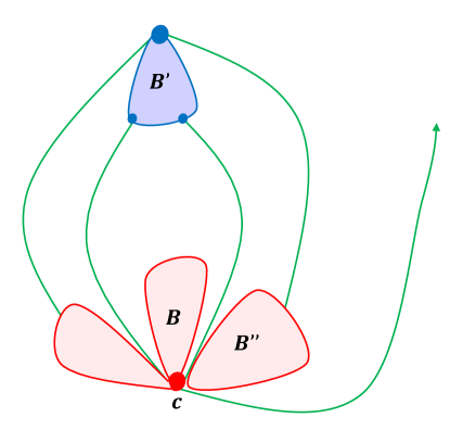
Figure 16: For the proof of Lemma 11: either $B^{\prime}$ or $B^{\prime\prime}$ is safe.

Consider the first case and refer to Fig. 16. Let $B^{\prime}$ be the block of both $u_{1}$ and $u_{2}$. Since the inner graph is plane, neither boundary edge of $B^{\prime}$ is incident to a vertex of $B$. Either $B^{\prime}$ is safe and we are done, or the boundary edges of $B^{\prime}$ are also incident to undrawn vertices of two blocks that have $c$ as their parent cutvertex. Again, either one of these blocks is safe and we are done, or their boundary edges must be incident to undrawn vertices of blocks whose least already-drawn ancestor is $u^{\prime}_{1}$. By repeating this argument, we find a block $B^{\prime\prime}$ having either $u^{\prime}_{1}$ or $c$ as its parent cutvertex and such that at least one boundary edge of $B^{\prime\prime}$ is incident to a vertex whose least already-drawn ancestor differs from both $u_{1}^{\prime}$ and $c$. Hence $B^{\prime\prime}$ is a safe block.

With similar reasoning, the existence of a safe block can be proved when $u_{1}$ and $u_{2}$ belong to different blocks with parent cutvertex $u^{\prime}_{1}=u^{\prime}_{2}$.∎

Safe moon. Suppose that $w$ is a parent cutvertex for a safe block $B$; for the moment we assume that $w$ is not on the separating cycle. Suppose that the parent block of $w$ is $B^{\prime}$; then $w$ has been drawn on the circular arc $\gamma(B^{\prime})$. Denote the circular disc defined by $\gamma(B^{\prime})$ by $\phi^{\prime}$. Let $\phi$ be a circular disc of radius $\epsilon_{2}$ with centre at $w$. We show how to choose $\epsilon_{2}$ later; for the moment we can assume that $\epsilon_{2}$ is very small in comparison to the radius of $\gamma(B^{\prime})$. The safe moon $\mu(w)$ for $w$ is the interior of $\phi-\phi^{\prime}$; see Fig.15(b).

Now we show how to choose $\epsilon_{2}$. Again let $\delta$ denote $d/n$, where $d$ denotes the minimum length of a side of the separating polygon, and $n$ is the number of vertices in the graph. Now consider two points $\alpha$ and $\alpha^{\prime}$ at distance $\frac{\delta}{2}$ from $u$. We choose $\epsilon_{2}$ small enough that: (i) $\mu(w)$ at $u$ does not intersect the tangents to $\gamma(B^{\prime})$ at $\alpha$ and $\alpha^{\prime}$; (ii) $\mu(w)$ does not intersect the line through $s$ and $t$. Small adjustments to this choice of $\mu(w)$ are required for the cases where $w$ is on the separating cycle, and where $w$ is an endpoint of $\gamma(B^{\prime})$.

A consequence of the definition of safe moon is the following: Let $w_{1}$ and $w_{2}$ be vertices on the circular arcs $\gamma(B_{1})$ and $\gamma(B_{2})$ for two blocks $B_{1}$ and $B_{2}$ that have been drawn. Let $\alpha_{1}$ be a point in $\mu(w_{1})$ and $\alpha_{2}$ be a point in $\mu(w_{2})$; the line segment between $\alpha_{1}$ and $\alpha_{2}$ does not intersect any safe moon other than $\mu(w_{1})$ and $\mu(w_{2})$.

Safe wedges. Suppose that the boundary edges of a non-root block $B$ are $e_{1}=(c,u_{1})$ and $e_{2}=(c,u_{2})$; let $u^{\prime}_{1}$ and $u^{\prime}_{2}$ be the vertices which are the least drawn ancestors of $u_{1}$ and $u_{2}$ respectively in their respective block-cutvertex trees. Since $B$ is safe, $u^{\prime}_{1}\not=u^{\prime}_{2}$. For each point $\alpha_{1}$ (resp. $\alpha_{2}$) in $\mu(u^{\prime}_{1})$ (resp. $\mu(u^{\prime}_{2})$), consider the wedge $\omega(\alpha_{1},\alpha_{2})$ formed by the rays from $c$ through $\alpha_{1}$ and $\alpha_{2}$. The safe wedge $\omega(B)$ of $B$ is the intersection of all such wedges $\omega(\alpha_{1},\alpha_{2})$ with the safe moon of $c$. This is illustrated in Fig. 17(a).

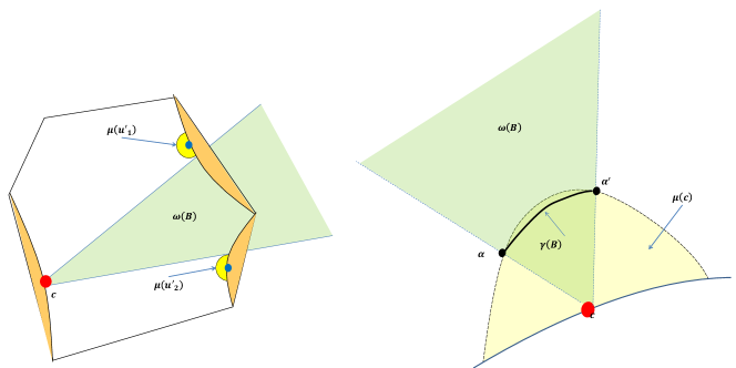
Figure 17: (a) A safe wedge. (b) The circular arc $\gamma(B)$.

The circular arc $\gamma(B)$. Suppose that $B$ is a non-root block. We give a location to each vertex in $B$ except the parent cutvertex $c$ (which is already drawn). These vertices are drawn on a circular arc $\gamma(B)$, defined as follows. Suppose that the boundaries of $\mu(c)$ and $\omega(B)$ intersect at points $\alpha$ and $\alpha^{\prime}$ as shown in Fig 17(b). Then $\gamma(B)$ is a circular arc that passes through $\alpha$ and $\alpha^{\prime}$. The radius of $\gamma(B)$ is chosen so that it lies inside $\mu(c)$, and it is distant at most $\epsilon_{1}$ from the straight line between $\alpha$ and $\alpha^{\prime}$. Here $\epsilon_{1}$ is chosen in exactly the same way as for the root block.

Putting it all together. In the construction of the inner graph in subsection 3.3, all vertices that are neither left nor right are removed, and the resulting non-triangular faces are fan-triangulated. These vertices can be drawn as follows. Each fan-triangulated face, after removal of the dummy edges, is star-shaped. The non-aligned vertices (neither left nor right) that came from this face form a triangulation inside the face. Thus we can use the linear-time algorithm of Hong and Nagamochi [9] to construct a straight-line drawing replacing the non-aligned vertices. This concludes the proof of sufficiency of Theorem 3.1.

4 Concluding Remarks

Assuming the real RAM model of computation, it can be proved that all algorithmic steps presented in the previous section can be executed in $O(n)$ time, where $n$ is the number of vertices of $G$.

Theorem 4.1

Let $G$ be an almost-planar $\mathbb{S}^{2}$-topological graph with $n$ vertices such that every vertex of $G$ is consistent. There exists an $O(n)$ time algorithm that computes an $\mathbb{S}^{2}$-embedding preserving straight-line drawing of $G$.

The real RAM model of computation allows for exponentially bad resolution in the drawing. The next theorem shows that such exponentially bad resolution is inevitable in the worst case. The construction of the family of almost-planar graphs for Theorem 4.2 is based on a family of upward planar digraphs first described by Di Battista et al. [2]. The graph $G_{1}$ is illustrated in Fig. 18(a), and for $k>1$, the graph $G_{k}$ is formed from $G_{k-1}$ as illustrated in Fig. 18(b).

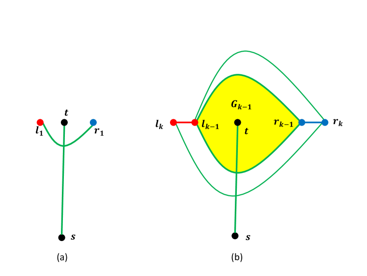
Figure 18: A family of graphs that require exponential area: (a) $G_{1}$; (b) Creating $G_{k}$ from $G_{k-1}$.

The graph $G_{5}$ is illustrated in Fig. 19.

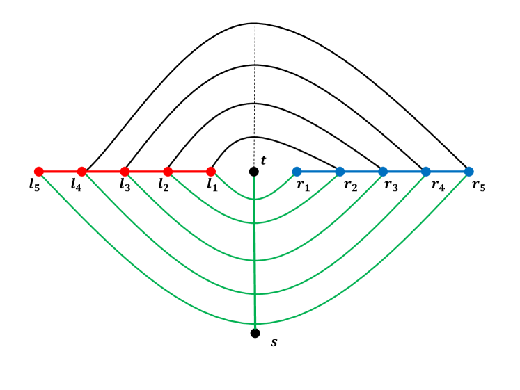
Figure 19: $G_{5}$.

Note that $G_{k}$ consists of a path $(\ell_{k},\ell_{k-1},\ldots,\ell_{1},r_{1},r_{2},\ldots,r_{k})$ and a number of chords on that path. Some chords cross $(s,t)$ and some do not. The chords form a kind of “spiral” path $(r_{1},\ell_{1},r_{2},\ell_{2},\ldots,r_{k-1},\ell_{k},r_{k})$, alternating between edges that cross $(s,t)$ and edges that do not.

It is easy to see (from Theorem 3.1) that $G_{k}$ has a straight-line drawing.

Theorem 4.2

For each $k\geq 1$, there is an almost-planar $\mathbb{S}^{2}$-topological graph $G_{k}$ with $2k+1$ vertices, such that any $\mathbb{S}^{2}$-embedding preserving straight-line drawing of $G_{k}$ requires area $\Omega(2^{k})$ under any resolution rule.

Proof

Firstly we orient the edges of $G_{k}$ to obtain an acyclic digraph. Consider Fig. 18(b). Note that $\ell_{i}$ is a left vertex and $r_{i}$ is a right vertex for each $i$; we orient edges from the left vertex to the right vertex. Also, we orient each edge $(\ell_{i},\ell_{i-1})$ from $\ell_{i-1}$ to $\ell_{i}$ and each edge $(r_{i},r_{i-1})$ from $r_{i}$ to $r_{i-1}$ ($1<i\leq k$).

Let $\overrightarrow{G}_{k}$ denote the resulting directed acyclic subgraph. Note that $\overrightarrow{G}_{k}$ is similar to the $n$-vertex graph used by Di Battista et al. [2] to show that upward planar drawings require $\Omega(4^{n})$ area; in fact deletion of the edge $(s,t)$, and the vertices $s$ and $t$, yields the Di Battista et al. graph.

Now suppose that the $\mathbb{S}^{2}$-topological graph $G_{k}$ has a straight-line drawing $\Gamma_{k}$. Assume w.l.o.g. that edge $(s,t)$ is vertical in $\Gamma_{k}$, and every left vertex $\ell_{i}$ is drawn in the left half-plane defined by the line through $(s,t)$.

The drawing $\Gamma_{k}$ has the same $\mathbb{S}^{2}$-embedding as $G_{k}$, but may have a number of different $\mathbb{R}^{2}$-embeddings, depending on the choice of the external face. Consider first the simplest case, where $\Gamma_{k}$ has the $\mathbb{R}^{2}$-embedding as shown in Fig.18(b). That is, the external face contains the vertices $s$, $\ell_{k}$, $r_{k}$, and $r_{k-1}$. We next show that, in this case, $\Gamma_{k}$ is an upward planar drawing.

For every vertex $\ell_{i}$ ($1<i<k$) in $\Gamma_{k}$, let $p$ be the point where edge $(r_{i},\ell_{i})$ crosses edge $(s,t)$, and let $q$ be the point where edge $(\ell_{i},r_{i+1})$ crosses the line through $(s,t)$. Similarly, let $p^{\prime}$ be the point where edge $(r_{i+1},\ell_{i+1})$ crosses the line through the edge $(s,t)$, and let $q^{\prime}$ be the point where edge $(\ell_{i+1},r_{i+2})$ crosses the line through the edge $(s,t)$.

Since $\Gamma_{k}$ has the same $\mathbb{R}^{2}$-embedding of $G_{k}$ in Fig.18(b), the triangle $(\ell_{i},p,q)$ is inside the triangle $(\ell_{i+1},p^{\prime},q^{\prime})$, sharing only a portion of the line through $s$ and $t$. Since this line is vertical, it follows that the $x$-coordinate of $\ell_{i+1}$ is smaller than the $x$-coordinate of $\ell_{i}$ in $\Gamma_{k}$. By a similar argument it can be proved that the $x$-coordinate of $r_{i}$ must be smaller than the $x$-coordinate of $r_{i+1}$ in $\Gamma_{k}$.

Hence the left-right subgraph has an upward drawing in $\Gamma_{k}$; from the Theorem of Di Battista et al. [2], the area is of $\Gamma_{k}$ is $\Omega(4^{2k+1})$; this is $\Omega(2^{k})$.

We now consider the more general case, where the external face of $\Gamma_{k}$ is not necessarily the same as in Fig.18(b). Since $\Gamma_{k}$ has the same $\mathbb{S}^{2}$-embedding as $G_{k}$, the external face of $\Gamma_{k}$ should include one of the faces of the graph $\hat{G}_{k}$ formed from $G_{k}$ by deleting the edge $(s,t)$. From Lemma 4, the external face cannot include an edge that crosses $(s,t)$; thus the external face must be $F_{j}=(\ell_{j-1},\ell_{j},r_{j+1},r_{j})$ for some $1<j<k$. As an example, the face $F_{3}$ is shown in Fig. 20.

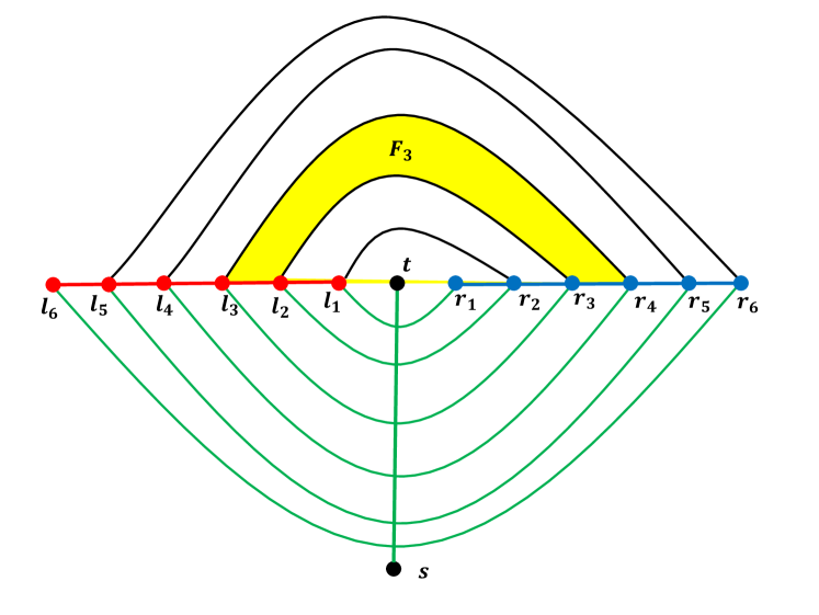
Figure 20: Face $F_{3}$ in $G_{6}$.

Now we consider two possibilities for the face $F_{j}$: $j>\frac{k}{2}$, and $j\leq\frac{k}{2}$.

If $j>\frac{k}{2}$, then we consider the subgraph of $G_{k}$ induced by $\{s,t\}\cup\{\ell_{j},\ell_{j-1},\ldots,\ell_{1}\}\cup\{r_{1},r_{2},\ldots,r_{j}\}$. This is isomorphic to $G_{j}$, and its external face contains $s$, $\ell_{j}$, $r_{j}$, and $r_{j-1}$. This corresponds to the “simplest case” described above, and so any straight-line drawing has area $\Omega(4^{2j+1})$; since $j>\frac{k}{2}$, this is $\Omega(2^{k})$.

Next consider the case that $j\leq\frac{k}{2}$. In Fig. 21 the $\mathbb{R}^{2}$-embedding where $j=3$ for $G_{6}$ is illustrated.

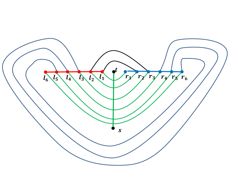
Figure 21: Using face $F_{3}$ from Fig. 20 as the external face.

In this case, consider the subgraph $H_{j,k}$ of $G_{k}$ induced by $\{s,t,\ell_{l},\ell_{k-1},\ldots,\ell_{j},r_{j},r_{j+1},\ldots,r_{k}\}$. The graph $H_{3,6}$ is illustrated in Fig. 22.

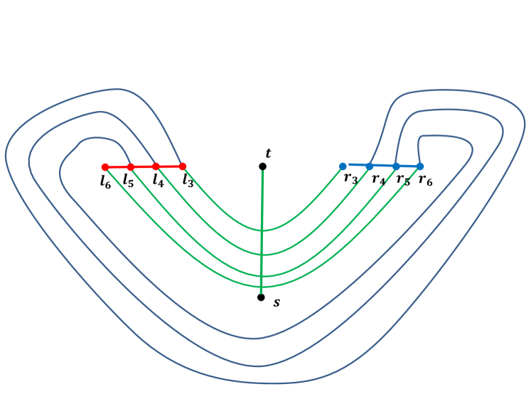
Figure 22: The graph $H_{3,6}$.

In fact $H_{j,k}$ is isomorphic to $G_{k-j}$. The graph $H_{3,6}$ is in Fig. 22 is re-drawn in Fig. 23 to illustrate the isomorphism.

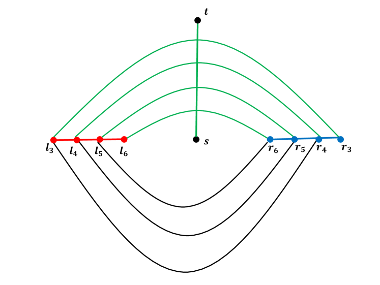
Figure 23: The graph $H_{3,6}$ redrawn to show the isomorphism with $G_{3}$.

Thus, using the same argument as in the simple case above, we can show that any straight-line drawing of $H_{j,k}$ has area $\Omega(4^{2(k-j)+1})$; since $j\leq\frac{k}{2}$, this is $\Omega(2^{k})$.

This completes the proof of Theorem 4.2.

We conclude this section by observing that the arguments used to prove Theorem 3.1 lead to a characterization of the maximal almost-planar $\mathbb{R}^{2}$-topological graphs that have $\mathbb{R}^{2}$-embedding preserving straight-line drawings.

Theorem 4.3

A maximal almost-planar $\mathbb{R}^{2}$-topological graph $G$ admits an $\mathbb{R}^{2}$-embedding preserving straight-line drawing of $G$ if and only if every vertex of $G$ is consistent, and every internal face of $G_{LR}$ is consistent.

Proof

The sufficiency of Theorem 4.3 is proved in Sections 3.3, 3.4, and 3.5. We show that the conditions of Theorem 4.3 are also necessary.

Suppose that $G_{LR}$ has an inconsistent face $f$, and has a straight-line drawing $\Gamma$. Now $f$ contains a cycle $C$ with at least one left vertex and at least one right vertex. From Lemma 4, $C$ contains $s$ and $t$, and the edge $(s,t)$. Further, since $G_{LR}$ has no edge that joins a left vertex to a right vertex, traversing $\Gamma$ in the clockwise direction from $t$ gives a polygonal chain $C_{L}$ of vertices, followed by $s$, followed by a polygonal chain $C_{R}$ of right vertices. All of $C_{L}$ is strictly to the left of the line through $s$ and $t$, and $C_{R}$ is strictly right of this line. This is only possible if the line segment between $s$ and $t$ lies inside $C$. However, the edge $(s,t)$ cannot lie inside $C$ because $f$ is a face of $G_{LR}$.

5 Open Problems

We mention two open problems that are naturally suggested by the research in this paper. The first open problem is about characterizing those almost-planar $\mathbb{R}^{2}$-topological graphs that admit an embedding preserving straight-line drawing. Theorem 4.3 provides such a characterization for the family of maximal almost-planar graphs.

The second open problem is about extending Theorem 3.1 to $k$-skew graphs with $k>1$. A topological graph $G=(V,E)$ is $k$-skew if there is a set $E^{\prime}\subset E$ of edges such that $G^{-}=(V,E-E^{\prime})$ has no crossings where $|E^{\prime}|\leq k$. Many graphs that arise in practice are $k$-skew for small values of $k$; this paper gives drawing algorithms for the case $k=1$. For each edge $e\in E^{\prime}$, one could define “left vertex relative to $e$” and “right vertex relative to $e$”, extending the definitions of left and right in this paper. However, it is not difficult to find a topological 2-skew graph in which all vertices are consistent with respect to the 2 “crossing” edges, but do not admit a straight-line drawing. It would be interesting to characterize $k$-skew graphs that admit a straight-line drawing for $k>1$.

References

- [1] Giuseppe Di Battista, Peter Eades, Roberto Tamassia, and Ioannis G. Tollis. Graph Drawing: Algorithms for the Visualization of Graphs. Prentice-Hall, 1999.
- [2] Giuseppe Di Battista, Roberto Tamassia, and Ioannis G. Tollis. Area requirement and symmetry display of planar upward drawings. Discrete & Computational Geometry, 7:381–401, 1992.
- [3] Sergio Cabello and Bojan Mohar. Adding one edge to planar graphs makes crossing number and 1-planarity hard. SIAM J. Comput., 42(5):1803–1829, 2013.
- [4] N .Chiba, T. Yamanouchi, and T. Nishizeki. Linear algorithms for convex drawings of planar graphs. Progress in Graph Theory, Academic Press, London, page 153 – 173, 1984.
- [5] Marek Chrobak and David Eppstein. Planar orientations with low out-degree and compaction of adjacency matrices. Theor. Comput. Sci., 86(2):243–266, 1991.
- [6] Peter Eades, Qing-Wen Feng, Xuemin Lin, and Hiroshi Nagamochi. Straight-line drawing algorithms for hierarchical graphs and clustered graphs. Algorithmica, 44(1):1–32, 2006.
- [7] Carsten Gutwenger, Petra Mutzel, and René Weiskircher. Inserting an edge into a planar graph. Algorithmica, 41(4):289–308, 2005.
- [8] Seok-Hee Hong, Peter Eades, Giuseppe Liotta, and Sheung-Hung Poon. Fáry’s theorem for 1-planar graphs. In Joachim Gudmundsson, Julián Mestre, and Taso Viglas, editors, COCOON, volume 7434 of Lecture Notes in Computer Science, pages 335–346. Springer, 2012.
- [9] Seok-Hee Hong and Hiroshi Nagamochi. Convex drawings of graphs with non-convex boundary constraints. Discrete Applied Mathematics, 156(12):2368–2380, 2008.
- [10] Michael Jünger and Sebastian Leipert. Level planar embedding in linear time. J. Graph Algorithms Appl., 6(1):67–113, 2002.
- [11] Hiroshi Nagamochi. Straight-line drawability of embedded graphs. Technical Report 2013-005, Graduate School of Informatics, Kyoto University, 2013.
- [12] Carsten Thomassen. Rectilinear drawings of graphs. Journal of Graph Theory, 12(3):335–341, 1988.