Skyrme Random-Phase-Approximation description of lowest $K^{\pi}=2^{+}_{\gamma}$ states in axially deformed nuclei

Abstract

The lowest quadrupole $\gamma$-vibrational $K^{\pi}=2^{+}$ states in axially deformed rare-earth (Nd, Sm, Gd, Dy, Er, Yb, Hf, W) and actinide (U) nuclei are systematically investigated within the separable random-phase-approximation (SRPA) based on the Skyrme functional. The energies $E_{\gamma}$ and reduced transition probabilities $B(E2)$ of $2^{+}_{\gamma}$-states are calculated with the Skyrme forces SV-bas and SkM^∗. The energies of two-quasiparticle configurations forming the SRPA basis are corrected by using the pairing blocking effect. This results in a systematic downshift of $E_{\gamma}$ by 0.3-0.5 MeV and thus in a better agreement with the experiment, especially in Sm, Gd, Dy, Hf, and W regions. For other isotopic chains, a noticeable overestimation of $E_{\gamma}$ and too weak collectivity of $2^{+}_{\gamma}$-states still persist. It is shown that domains of nuclei with a low and high $2^{+}_{\gamma}$-collectivity are related with the structure of the lowest 2-quasiparticle states and conservation of the Nilsson selection rules. The description of $2^{+}_{\gamma}$ states with SV-bas and SkM^∗ is similar in light rare-earth nuclei but deviates in heavier nuclei. However SV-bas much better reproduces the quadrupole deformation and energy of the isoscalar giant quadrupole resonance. The accuracy of SRPA is justified by comparison with exact RPA. The calculations suggest that a further development of the self-consistent calculation schemes is needed for a systematic satisfactory description of the $2^{+}_{\gamma}$ states.

I Introduction

During the last decades, remarkable progress was made in description of nuclear dynamics within self-consistent mean-field (SCMF) models (Skyrme, Gogny, relativistic), see e.g. the reviews Ben03 ; Vre05 ; Pa07 ; Er10 . In particular, a variety of quasiparticle random-phase-approximation (QRPA) methods was developed for the exploration of small-amplitude excitations in deformed nuclei, Ne06 ; Yosh08 ; Arte08 ; Losa10 ; Ter10 ; Terasaki_PRC_11 ; Peru08 ; Peru11 ; Inakura09 ; Fracasso12 ; Hinohara13 . So far these methods were mainly used for the description of giant resonances (GR) in light Yosh08 ; Arte08 ; Losa10 ; Ter10 ; Peru08 ; Inakura09 ; Fracasso12 ; Hinohara13 and medium/heavy Ne06 ; Ter10 ; Peru11 ; Fracasso12 ; IJMPE_08 ; kle_PRC_08 ; Kva_EPJA13 ; Ve09 nuclei. However, self-consistent QRPA was still rarely employed for the exploration of the lowest vibrational states ($\beta$-, $\gamma$-, octupole) in deformed rare-earth and actinide nuclei Terasaki_PRC_11 ; Peru11 (despite rich available experimental information for these regions bnl_exp ; Sol_Grig ). This is partly due to the huge configuration spaces required for such deformed heavy nuclei. However, the main problem lies in a high sensitivity of the lowest vibrational states (LVS) to various factors. Following early calculations within the schematic Quasiparticle-Phonon Model (QPM) Sol76 ; Sol_Shir ; Sol_Sush_Shir , the description of LVS requires a proper treatment of the single-particle (s-p) spectra near the Fermi level, equilibrium deformation, pairing with the blocking effect, residual interaction (with both particle-hole and particle-particle channels), coupling to complex configurations (with taking into account the Pauli principle), and exclusion of the spurious admixtures. Besides, the description of LVS should be consistent with the treatment of other collective modes, e.g. multipole GR. All these factors and requirements make the self-consistent description of LVS very demanding.

So far we are aware of two self-consistent QRPA studies of LVS in rare-earth and actinide regions, one with Gogny forces for ²³⁸U Peru11 and another with Skyrme forces for rare-earth nuclei Terasaki_PRC_11 . Actually only the last study Terasaki_PRC_11 is systematic. It covers $\gamma$-vibrational $K^{\pi}=2^{+}_{\gamma}$ and $\beta$-vibrational $K^{\pi}=0^{+}_{\beta}$ states in 27 rare-earth nuclei. The Skyrme forces SkM^∗ SkMs and SLy4 SLy4 are used and performance of SkM^∗ is found noticeably better than of SLy4. It is deduced that Skyrme QRPA is a reasonable basis for the investigation of LVS.

In the present paper, we continue the systematic exploration of $2^{+}_{\gamma}$-states in axial deformed nuclei with QRPA using Skyrme forces. The $2^{+}_{\gamma}$-states are chosen as the simplest case where we do not meet the problem of the extraction of the spurious admixtures. As compared to Terasaki_PRC_11 , our study has some important new aspects.

First, it is desirable to use for description of $2^{+}_{\gamma}$-states the Skyrme forces which simultaneously reproduce the energy of the isoscalar giant quadrupole resonance (ISGQR). Following IJMPE_08 , these forces should have a large isoscalar effective mass $m^{*}_{0}/m$. The forces from Terasaki_PRC_11 have low effective masses, $m^{*}_{0}/m=$0.70 for SLy4 SLy4 and 0.79 for SkM^∗ SkMs , and so overestimate the ISGQR energy, see IJMPE_08 and discussion below. To make the description of ISGQR and $2^{+}_{\gamma}$-states consistent, we use in our calculations the recent SV-bas force SV with $m^{*}_{0}/m$=0.9. As shown below, SV-bas also manages to reproduce systematically well ground state deformations, a feature which is utterly crucial for a correct placing of LVS. Note that very similar results were earlier obtained nest_arXive15 with the Skyrme force SV-mas10 SV ($m^{*}_{0}/m$=1.0). We choose here SV-bas as a more general parametrization which was already used in various studies, see e.g. Er10 ; Kva_EPJA13 ; Ve09 ; Pot10 . For comparison with Terasaki_PRC_11 , the force SkM^∗ is also implemented.

Second, we take into account the pairing blocking effect (PBE) Sol76 ; Eisenberg-book ; Ri80 ; Nilsson-book ; BCS50 which, following QPM studies Sol76 ; Sol_Shir ; Sol_Sush_Shir , can be important for QRPA description of LVS in axially deformed nuclei. The PBE weakens the pairing and thus downshifts energies of low-energy two-quasiparticle (2qp) states by a few hundreds keV Sol76 ; Sol_Shir ; Sol_Sush_Shir , which in turn decreases the QRPA energies of $2^{+}_{\gamma}$-states. This effect can be especially important for slightly collective states (with one or two dominant 2qp components) which are often encountered amongst $2^{+}_{\gamma}$-states. We implement PBE within the Bardeen-Cooper-Schrieffer (BCS) scheme using volume pairing Ben00 . The same volume pairing, though in the framework of the Hartree-Fock-Bogoliubov (HFB) approach without PBE, was used in Terasaki_PRC_11 .

In fact, we are taking from the PBE only one aspect, namely the modification of 2qp energies. The 2qp states as such (s.p. wave functions and pairing occupation amplitudes) remain untouched. This ad hoc solution to the problem with the energies of $2^{+}_{\gamma}$-states is admittedly not consistent. However it has a great advantage not to disturb the orthonormality of 2qp basis and thus allows to use the standard QRPA procedure. At the same time, following previous schematic Sol76 ; Sol_Shir ; Sol_Sush_Shir and our present studies, the PBE for $2^{+}_{\gamma}$-states in medium and heavy deformed nuclei can be strong and certainly deserves the consideration. In this connection, our PBE-QRPA calculations can be viewed as a first step highlighting the problem and calling for further checking within a self-consistent PBE-QRPA prescription, yet to be developed.

The third new aspect is that we provide a detailed analysis of the obtained results, both numerically and analytically (e.g. in terms of simplified models for schematic RPA). We determine domains of nuclei with low and high collectivity of $2^{+}_{\gamma}$-states and demonstrate that the lowest $K^{\pi}=2^{+}$ 2qp state plays a key role in formation of these domains. The study embraces 9 isotopic chains (Nd, Sm, Gd, Dy, Er, Yb, Hf, W, U) with 41 axially deformed nuclei, as compared to 27 rare-earth nuclei in Terasaki_PRC_11 .

The calculations are performed within the separable random-phase-approximation (SRPA) method based on the Skyrme functional Ben03 ; Skyrme ; Vau . The method is developed in a one-dimensional (1D) version for spherical nuclei Ne02 and a two-dimensional (2D) version Ne06 ; Ne_ar05 for axial deformed nuclei. SRPA is derived self-consistently: i) both the mean field and residual interaction are obtained from the same Skyrme functional, ii) the residual interaction includes all terms of the Skyrme functional as well as the Coulomb (direct and exchange) terms. The self-consistent factorization of the residual interaction dramatically reduces the computational effort for deformed nuclei while keeping high accuracy of the method. However SRPA is not self-consistent in the part of the pairing interaction because i) ad hoc implementation of PBE into QRPA and ii) skipping the particle-particle channel in the residual interaction.

In earlier studies, SRPA was successfully applied for the description of various GR in spherical and deformed nuclei: E1(T=1) and E2(T=0) Ne06 ; IJMPE_08 ; Ne02 ; kle_PRC_08 , toroidal/compression E1 Kva_EPJA13 , and spin-flip M1 Ve09 ). However, the success of the model for GR does not mean that it is also robust in description of so fragile excitations as LVS. In this connection, we compare below some SRPA results with those obtained with the exact (no the separable ansatz) 2D QRPA code repko . We find a nice agreement which confirms that SRPA is accurate enough to pretend for description of $2^{+}_{\gamma}$ states.

The paper is organized as follows. In Sec. 2, method and calculational details are outlined. The equations for the pairing blocking are given, the SRPA scheme is sketched, and SRPA results are compared with those from the exact QRPA. It is shown that SV-bas, unlike SkM*, nicely reproduces equilibrium quadrupole deformations and the ISQGR energy. Sec. 3 presents the main results for energies and reduced transition probabilities B(E2) of $2^{+}_{\gamma}$-states. In Sec. 4, these results are discussed and analyzed in detail and compared with the previous data Terasaki_PRC_11 . A summary is given in Sec. 5. In Appendix A, the expression for the pairing matrix element is derived. In Appendix B, the basic SRPA equations are outlined. In Appendix C, a simple two-pole RPA model is presented to be applied for explanation of the domains with low and high collectivity of $2^{+}_{\gamma}$-states. In Appendix D, SRPA strength constants of the residual interaction are compared with those of the QPM.

II Model and calculation scheme

The SRPA approach Ne06 used in this paper is based on the Skyrme functional Ben03

$$\mathcal{E}(\rho,\tau,\bf{J},\bf{j},\bf{\sigma},\bf{T})=\mathcal{E}_{\rm{kin}}+\mathcal{E}_{\rm{Sk}}+\mathcal{E}_{\rm{Coul}}+\mathcal{E}_{\rm{pair}}$$ (1)

where $\mathcal{E}_{\rm{kin}}$ is the kinetic energy, $\mathcal{E}_{\rm{Sk}}$ is the potential energy according to the Skyrme functional, $\mathcal{E}_{\rm{Coul}}$ is the Coulomb energy, and $\mathcal{E}_{\rm{pair}}$ is the pairing energy. The Coulomb exchange term is treated in Slater approximation. The volume pairing corresponds to a zero-range pairing interaction. The Skyrme part $\mathcal{E}_{\rm{Sk}}$ depends on the local densities and currents: density $\rho(\mathbf{r})$, kinetic-energy density $\tau(\mathbf{r})$, spin-orbit density $\mathbf{J}(\mathbf{r})$, current $\mathbf{j}(\mathbf{r})$, spin-density $\mathbf{\sigma}(\mathbf{r})$, and spin-kinetic-energy density $\mathbf{T}(\mathbf{r})$ Ben03 . The mean-field Hamiltonian and SRPA residual interaction are self-consistently determined through the first and second functional derivatives of (1), respectively Ne06 . Further details of the model and calculation scheme are given below.

II.1 Mean field and quadrupole deformation

The stationary 2D mean-field calculations are performed with the SKYAX code SKYAX in cylindrical coordinates using a mesh size of 0.5 fm and a box size of about three nuclear radii. The single-particle space is chosen to embrace the levels from the bottom of the potential well up to energy 15-20 MeV. For SV-bas, the s-p schemes involve 304 proton and 375 neutron levels in ¹⁵⁰Nd and 379 proton and 485 neutron levels in ²³⁸U.

The ground state is obtained by solving the mean-field equations and resides at the minimum of the total energy (1). Its axial quadrupole deformation is characterized by the dimensionless deformation parameter Raman

$$\beta_{2}=\sqrt{\frac{5\pi}{3}}\frac{Q_{2}}{ZR^{2}},$$ (2)

where $Q_{2}=\int d{\mathbf{r}}\rho_{p}({\mathbf{r}})r^{2}Y_{20}$ is the quadrupole moment, $R=1.2\;\rm{fm}A^{1/3}$, A is the mass number.

Figure 1 compares deformation parameters calculated using SV-bas with available experimental data bnl_exp and Fig. 2 shows the same comparison for SkM^∗. Figures 1 and 2 show very nice agreement for SV-bas while SkM^∗ systematically overestimates $\beta_{2}$, especially in Yb, Hf, W, and U isotopes. Note that both SV-bas and SkM^∗ fail to describe the specifically low values of experimental $\beta_{2}$ in ¹⁷⁰Yb and ^172,174Hf. Note also the exceptionally large error bars in ¹⁷⁰Hf.

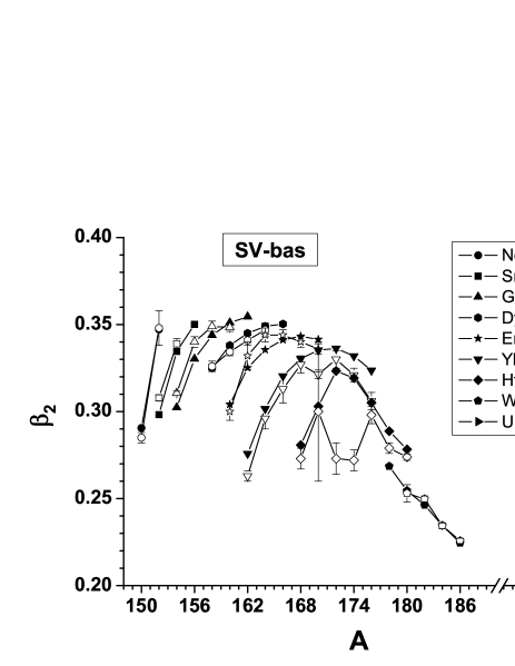
Figure 1: Parameter $\beta_{2}$ of the axial quadrupole deformation in rare-earth and actinide nuclei. The values calculated with SV-bas SV (full symbols) are compared with the experimental data bnl_exp (open symbols with error bars).

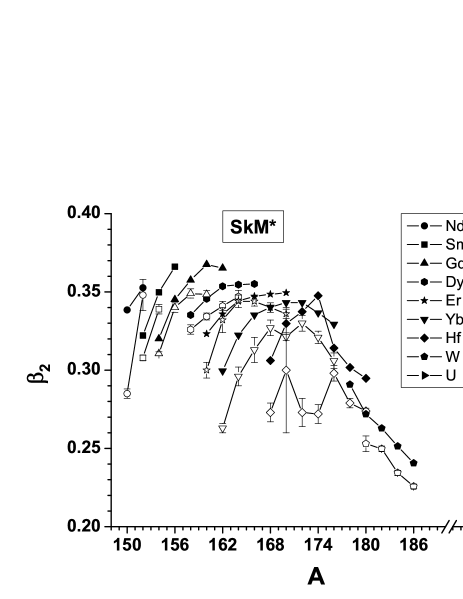
Figure 2: The same as Fig. 1 but for SkM^∗.

II.2 Pairing and blocking effect

The volume pairing interaction reads

$$V^{q}_{\rm{pair}}({\mathbf{r}},{\mathbf{r}}^{\prime})=V_{q}\>\delta(\mathbf{r}-\mathbf{r}^{\prime}),$$ (3)

where $q$ stands for protons or neutrons and $V_{q}$ are pairing strengths. In the present study pairing is treated at the BCS level Ben00 .

If the pairing-blocking effect (PBE) is accounted for, the BCS problem is solved separately for the ground $\Psi_{0}^{q}$ and excited n-quasiparticle $\Psi_{n}^{q}$ states. For the ground state, the expectation value $\langle\Psi_{0}^{q}|H_{\rm{pair}}|\Psi_{0}^{q}\rangle$ for the pairing Hamiltonian $H_{\rm{pair}}$ is minimized to determine the set of Bogoliubov coefficients $\{u_{k}^{q},v_{k}^{q}\}$. For $n$-quasiparticle excitation, the wave function reads

$$\Psi_{n}^{q} = \hat{\alpha}^{+}_{j_{1}}...\hat{\alpha}^{+}_{j_{n}}\Psi_{0}^{q}=\hat{a}^{+}_{j_{1}}...\hat{a}^{+}_{j_{n}}$$

$$\cdot \prod_{k\neq j_{1}...j_{n}\in q}[u_{k}^{q}(j_{1}...j_{n})+v_{k}^{q}(j_{1}...j_{n})\hat{a}^{+}_{k}\hat{a}^{+}_{\bar{k}}]|-\rangle,$$

where $\hat{a}^{+}_{j}(\hat{\alpha}^{+}_{j})$ creates the particle (quasiparticle) at the state $j$ and $|-\rangle$ is the particle vacuum. For this excitation, the expectation $\langle\Psi_{n}^{q}|H_{\rm{pair}}|\Psi_{n}^{q}\rangle$ is minimized and the new set of occupation numbers $\{u_{k}^{q}(j_{1},..j_{n}),v_{k}^{q}(j_{1},..j_{n})\}$ specific for the given excitation is determined. In the latter case, the BCS equations for axially deformed nuclei (with doubly degenerate s-p levels) have a peculiarity: if some states from the set $\{j_{1},...j_{n}\}$ are unpaired, then these states are excluded from the pairing scheme and contribute to the BCS equations as pure single-particle states. The physics behind is obvious: if some level is occupied by an unpaired nucleon, then it is closed (=blocked) for the pairing process which transfers nuclear pairs. This is why it is called pairing blocking effect Sol76 ; Eisenberg-book ; Ri80 ; Nilsson-book ; BCS50 .

The PBE takes place in both BCS and HFB theories as soon as we deal with n-quasiparticle excitations. Most often the PBE is considered for 1qp excitations in odd and odd-odd nuclei, see e.g. Ben00 ; Dug01 ; Pot10 and more references in BCS50 . Following QPM studies Sol76 ; Sol_Shir ; Sol_Sush_Shir , the PBE may play a role in QRPA description of LVS in even-even axially deformed nuclei. Indeed 2qp states constitute the configuration space for QRPA. The first low-energy 2qp states are the main contributors to the lowest QRPA excitation. So it is worth to check how PBE for the low-energy 2qp states affects the description of LVS.

The main effect of the PBE is to change the 2qp energies Sol76 ; Sol_Shir ; Sol_Sush_Shir . Thus we use here in ad-hoc manner only one PBE output, PBE-corrected 2qp energies. Only them are implemented to QRPA while the occupation amplitudes ($u,v$) and s.p. wave functions are kept the same as in the BCS ground state. This has the advantage that orthonormality of the 2qp configuration space is maintained and the standard QRPA scheme remains applicable.

Usually in BCS+QRPA calculations the 2qp-energies are computed by using the pairing gaps $\Delta_{q}$, chemical potentials $\lambda_{q}$ and Bogoliubov coefficients $\{u_{k}^{q},v_{k}^{q}\}\in q$ for the ground BCS state, yielding

$$\epsilon_{ij}^{q}=\epsilon_{i}^{q}+\epsilon_{j}^{q}$$ (5)

where $\epsilon_{i}^{q}=\sqrt{(\tilde{e}_{i}^{q}-\lambda_{q})^{2}+\Delta_{q}^{2}}$ is the energy of the 1qp state, $\tilde{e}_{i}^{q}$ is the renormalized s-p energy (see the expression below). In HFB+QRPA calculations, the 2qp states for the QRPA configuration space are also expressed in terms of ground state values. In particular, their energies are calculated as a sum of two 1qp energies in the canonical basis using the HFB solutions for the ground state, see e.g. Ter10 ; Terasaki_PRC_11 ; Peru11 . Both such BCS and HFB schemes do not include the PBE for the 2qp states. Following QPM and our calculations, such a treatment can be insufficient for a correct description of the LVS.

For $K^{\pi}=2^{+}$ states

$$\Psi^{q}(ij) = \hat{\alpha}^{+}_{i}\hat{\alpha}^{+}_{j}\Psi_{0}^{q}$$

$$= \hat{a}^{+}_{i}\hat{a}^{+}_{j}\prod_{k\neq i,j\in q}(u_{k}^{q}(ij)+v_{k}^{q}(ij)\hat{a}^{+}_{k}\hat{a}^{+}_{\bar{k}})|-\rangle,$$

the 2qp pairs are necessarily non-diagonal ($i\neq j$). For a constant pairing force, the BCS-PBE prescription for this case was formulated in Sol76 . Below we present the BCS-PBE formalism for the $\delta$-force volume pairing (3). For each 2qp state $\Psi^{q}(ij)$, one should solve the system of BCS+PBE equations

$$[u_{k}^{q}(ij)]^{2}=\frac{1}{2}\>\left\{1+\frac{\tilde{e}_{k}^{q}-\lambda_{q}(ij)}{\sqrt{\left[\tilde{e}_{k}^{q}-\lambda_{q}(ij)\right]^{2}+[\Delta_{k}^{q}(ij)]^{2}}}\right\},$$ (7)

$$[v^{q}_{k}(ij)]^{2}=\frac{1}{2}\>\left\{1-\frac{\tilde{e}_{k}^{q}-\lambda_{q}(ij)}{\sqrt{\left[\tilde{e}_{k}^{q}-\lambda_{q}(ij)\right]^{2}+[\Delta_{k}^{q}(ij)]^{2}}}\right\},$$ (8)

$$\Delta_{k}^{q}(ij)=-\sum_{k^{\prime}\neq i,j}^{K^{\prime}>0,k^{\prime}\in q}f_{k^{\prime}}^{q}V^{(\rm{pair,q})}_{k\bar{k}k^{\prime}\bar{k^{\prime}}}\>v_{k^{\prime}}^{q}(ij)u_{k^{\prime}}^{q}(ij),$$ (9)

$$N_{q}=2+\sum_{k^{\prime}\neq i,j}^{K^{\prime}>0,k^{\prime}\in q}f_{k^{\prime}}^{q}\left\{1-\frac{\tilde{e}_{k}^{q}-\lambda_{q}(ij)}{\sqrt{\left[\tilde{e}_{k}^{q}-\lambda_{q}(ij)\right]^{2}+[\Delta_{k}^{q}(ij)]^{2}}}\right\},$$ (10)

where

$$\tilde{e}_{k}^{q}=e_{k}^{q}-1/2\sum_{k^{\prime}\in q}f_{k^{\prime}}^{q}V^{(\rm{pair,q})}_{k\bar{k}k^{\prime}\bar{k^{\prime}}}[v_{k}^{q}]^{2}$$ (11)

is the renormalized s-p energy and $e_{k}^{q}$ is the initial s-p energy. Furthermore, $u_{k}^{q}(ij),v_{k}^{q}(ij),\Delta_{k}^{q}(ij),\lambda_{q}(ij)$ are Bogoliubov coefficients, pairing gaps and chemical potentials, calculated for the 2qp $(ij)$-excitation. The sums in (9) and (10) include all s-p states $k^{\prime}$ (with isospin $q$ and projection $K^{\prime}>0$ of the total angular momentum) for exception of $k^{\prime}=i$ and $j$; $N_{p}=Z$ and $N_{n}=N$ are proton and neutron numbers. The smoothing energy-dependent cut-off weights $f_{k^{\prime}}^{q}$ are introduced to cure the well-known drawback of the zero-range pairing force to overestimate the coupling to the (continuum) high-energy states Ri80 ; BCS50 . Expressions for weights $f_{k^{\prime}}^{q}$ and pairing matrix elements $V_{k\bar{k}k^{\prime}\bar{k^{\prime}}}^{(\rm{pair,q})}$ in axial nuclei are given in the Appendix A.

The PBE-corrected energy of the 2qp excitation reads

$$\mathcal{E}^{q}_{\rm{bl}}(ij)=\mathcal{E}^{q}(ij)-\mathcal{E}^{q}_{0}$$ (12)

where

$$\mathcal{E}^{q}_{\rm{bl}}(ij)=\langle\Psi^{q}(ij)|H^{q}_{\rm{pair}}|\Psi^{q}(ij)\rangle=\tilde{e}^{q}_{i}+\tilde{e}^{q}_{j}+$$ (13)

$$\quad+\sum_{k\neq i,j}^{K>0,k\in q}f^{q}_{k}[2\tilde{e}^{q}_{k}\>(v^{q}_{k}(ij))^{2}-\Delta_{k}^{(q)}(ij)\>u^{q}_{k}(ij)\>v^{q}_{k}(ij)]$$

is the energy of the system in the (ij)-state and

$$\mathcal{E}^{q}_{0} = \langle\Psi^{q}_{0}|H^{q}_{\rm{pair}}|\Psi^{q}_{0}\rangle$$

$$= 2\sum_{k}^{K>0,k\in q}f^{q}_{k}\tilde{e}^{q}_{k}\>(v^{q}_{k})^{2}-\sum_{k}^{K>0,k\in q}f^{q}_{k}\Delta^{q}_{k}\>u^{q}_{k}\>v^{q}_{k}\;,$$

is the energy of the q-subsystem in the ground state. The values $u_{k},v_{k},\Delta_{k}^{q},\lambda_{q}$ in (II.2) are for the ground state. Eqs. (9), (10), (13) show that PBE excludes the states $i$ and $j$ from the pairing sums. These blocked states do not contribute to the pairing gap (9) and enter (10) and (13) as single-particle (not quasi-particle) states.

The sums in (9), (10), and (13) are usually dominated by a few $k^{\prime}$-states around the Fermi level. If the states $i$ and $j$ belong to this group, then their blocking can effectively decrease the level density near the Fermi level and thus the pairing gap (9). Consequently the energy (13) is changed. In such cases, the pairing is significantly suppressed and the BCS-PBE value for the 2qp energy(12) becomes a few hundreds of keV smaller than the BCS energy (5) Sol76 . This in turn leads to a significant downshift of the energy of the first QRPA solution.

In the present study, we block the five lowest $K^{\pi}=2^{+}$ 2qp states (proton and neutron altogether). The calculations show that this number of blocked states is optimal. More blocking would involve the states remote by energy from the Fermi level and thus with a negligible PBE. Less blocking is likely to miss a part of the PBE corrections.

We substitute the PBE-corrected energies $\mathcal{E}^{q}_{\rm{bl}}(ij)$ to SRPA replacing the $\epsilon^{q}_{ij}$. However we do not use the PBE modified Bogoliubov coefficients $\{u^{q}_{k}(ij),v^{q}_{k}(ij)\}$. Instead we continue to employ in QRPA the ground state set $\{u^{q}_{k},v^{q}_{k}\}$ and wave functions. This leaves the 2qp basis orthonormalized and renders our PBE-SRPA scheme easily applicable.

It is also worth to inspect a possible impact of our scheme on the basic features of QRPA, namely stability of the QRPA interaction matrix, elimination of spurious modes, and sum rules: i) Concerning the QRPA matrix, the PBE-induced reduction of the positive diagonal elements (2qp energies) of the matrix indeed can cause instabilities in some cases. This is checked numerically. We find that for the $K^{\pi}=2^{+}$ states studied here the QRPA remains in the stable regime. The only exception is ¹⁶⁴Dy in the calculations with the force SkM*, see discussion below. ii) Spurious modes must be carefully checked when trying to apply the PBE to other quadrupole states, say with $K^{\pi}=0^{+}$ and $K^{\pi}=1^{+}$, but not in our case. For $K^{\pi}=2^{+}$ states considered in the present study the spurious modes are absent at all. iii) Concerning the sum rules, there is some quantitative effect. But it is extremely small as the main contribution to sum rules comes from higher lying states which are not affected by the PBE. Altogether, the present ad hoc implementation of the PBE looks robust. It still calls for a thorough formal self-consistent development which, however, will be tedious and take time. We consider the present study as a first step in exploration of the impact of the PBE on low-lying spectra of $K^{\pi}=2^{+}$ states.

The PBE should be applied with care in case of a weak pairing because the blocking reduces pairing and may trigger its full break-down. In the worst case, a more involved formalism (allowing a weak pairing) should be used, e.g. the method with particle-number projection before variation Kuz . Calculations with this method show that BCS-PBE somewhat underestimates the 2qp energies Kuz . However, the projection method requires a huge effort and it cannot be consistently applied for Skyrme energy functional Dob07 . So we use here BCS-PBE, though with staying alert for suspect cases.

II.3 SRPA scheme

The SRPA formalism for axial nuclei is described in detail elsewhere Ne06 ; Ne_ar05 . Here we sketch only the points relevant for the present study. As mentioned above, the SRPA formalism starts from the functional (1). The residual interaction includes contributions from both time-even and time-odd densities and also takes care of the Coulomb interaction. The coupling between the quadrupole $\lambda\mu$=22 and hexadecapole $\lambda\mu$=42 modes, pertinent to deformed nuclei, is included. The basic SRPA equations and more calculation details can be found in the Appendix B.

The present SRPA version skips the particle-particle (hole-hole) channel for $K^{\pi}=2^{+}$ states. In QPM the pp-channel is used to harmonize description of LVS energies and transition probabilities Sol_Sush_Shir but these calculations are not self-consistent. The self-consistent Skyrme BCS-QRPA calculations for spherical nuclei show that the pp-channel tends to decrease the LVS energies Sev08 . If so, then this effect can be partly compensated by the energy upshift gained by using the particle-projection method Kuz . The Skyrme HFB-QRPA studies of LVS in deformed nuclei use the pp-channel only partly Terasaki_PRC_11 if at all Ter10 . In general, the pp-channel, being crucial for $\beta$-vibrational $K^{\pi}=0^{+}$ states, seems not to be so important for $\gamma$-vibrational $K^{\pi}=2^{+}$ states. At least we do not know any self-consistent study for the lowest $K^{\pi}=2^{+}$ states in axial deformed nuclei, which would demonstrate a real need for this channel.

In the present study, we calculate the structure and energies of the first RPA one-phonon $2^{+}_{\gamma}$ states ($\lambda\mu\nu=221$) in Nd, Sm, Gd, Dy, Er, Yb, Hf, W, and U isotopes. The reduced probability B(E2)=$|\langle\nu=1|\sum^{Z}_{k=1}r_{k}^{2}Y_{22}(\theta_{k})|0\rangle|^{2}$ of the transition from the ground $|0\rangle$ to the SRPA $\nu=1$ state are also computed.

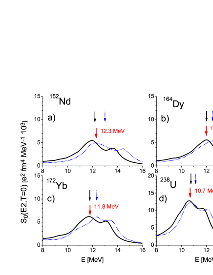
Figure 3: (Color online) The isoscalar strength function for the ISGQR in ¹⁵²Nd ¹⁶⁴Dy, ¹⁷²Yb and ²³⁸U, calculated with the Skyrme forces SkM^∗ SkMs (dotted blue line) and SV-mas10 SV (solid black line). The Lorentz averaging parameter is $\Delta$ = 1 MeV. The empirical estimations for the ISGQR centroids Scamps_PRC_13 are marked by lower red arrows with indicated energies. The SV-bas and SkM^∗ estimations for the centroids are denoted by upper black solid and blue dotted arrows, respectively.

The configuration space for $\lambda\mu=22$ involves, depending on the isotope, 6600-9600 proton and 9400-14200 neutron 2qp-states with excitation energies up to 55-80 MeV. This basis is sufficient for our aims. It results (together with the quadrupole components $\lambda\mu$=20 and 21) in a reasonable exhaustion of the total energy-weighted sum rule EWSR(E2,T=0)= $(\hbar^{2}e^{2})/(8\pi m_{p})50A\langle r^{2}\rangle_{A}$ by $\sim 95-98\%$. A similar size of configuration space was used in Terasaki_PRC_11 and Peru11 (19000-28000 and 23000-26000 2qp states, respectively).

The calculations are performed for the Skyrme parametrizations SV-bas and SkM^∗. As mentioned in the introduction, SV-bas is chosen because it provides an accurate description of the ground state deformations and ISGQR energies. This is demonstrated in Fig. 3, where ISGQR strength functions and energy centroids (see definitions in the Appendix B) are depicted for SV-bas and SkM^∗. The calculated centroids are 12.2 and 13.0 MeV in ¹⁵²Nd, 12.0 and 12.5 MeV in ¹⁶⁴Dy, 11.8 and 12.3 MeV in ¹⁷²Yb, and 10.7 and 11.1 MeV in ¹⁵²U, for SV-bas and SkM^∗ respectively. These results are compared with the empirical polynomial estimations Scamps_PRC_13 . It is seen that SV-bas well describes the energy centroids while SkM^∗ systematically overestimates them. So SV-bas demonstrates a good reproduction of both axial deformations and ISGQR energies which makes SV-bas a promising candidate for the description of $\gamma$-vibrational states.

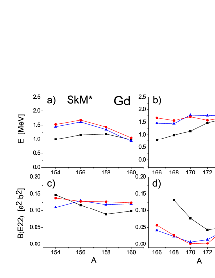
Figure 4: (Color online) Energies (a-b) and B(E2) values (c-d) of the $2^{+}_{\gamma}$-vibrational states, calculated with the force SkM^∗ in the framework of SRPA (red circles) and exact eRPA (blue triangles) in Gd (left) and Yb (right) isotopes. In both calculations, the PBE and pp-channel in the residual interaction are omitted. The experimental data bnl_exp are depicted by black squares.

To demonstrate the accuracy of SRPA, we compare in Fig. 4 some results for $K^{\pi}=2^{+}_{\gamma}$ states obtained within SRPA and exact 2D QRPA repko . The exact method is noted as eRPA. In both cases, the calculations are performed without PBE and pp-channel in the residual interaction. The isotopic chains with a high (Gd) and low (Yb) collectivity of $2^{+}_{\gamma}$ states are considered. We see a very nice agreement between SRPA and eRPA results, which demonstrates the robustness of SRPA. Since SRPA calculations require much less computational effort than eRPA, just SRPA is used in the following.

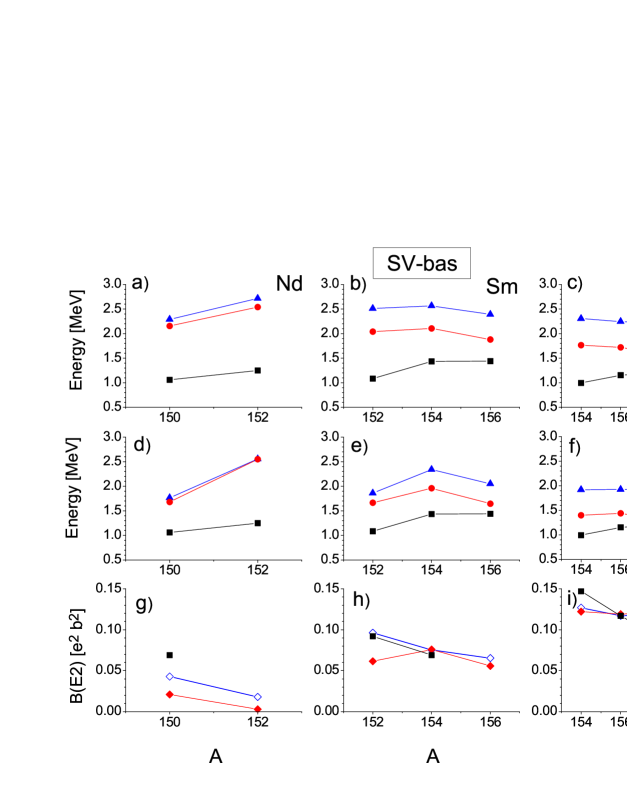
Figure 5: (Color online) The lowest 2qp and QRPA(RPA) energies (a-f) as well as B(E2) values (g-i) of 2${}^{+}_{\gamma}$-vibrational states in Nd (left), Sm (center) and Gd (right) isotopes, calculated with the force SV-bas. The 2qp (filled blue triangles) and QRPA(RPA) (filled red circles) energies are obtained without (a-c) and with (d-f) PBE. The QRPA(RPA) B(E2) values without (empty blue diamonds) and with (filled red diamonds) PBE are plotted in (g-i). In all the plots, the experimental data bnl_exp are given (filled black squares).

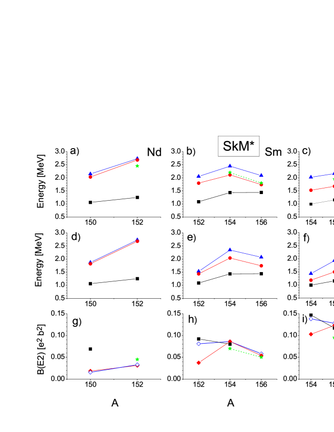
Figure 6: (Color online) The same as in Fig. 5 but for SkM^∗. For the comparison, the SkM^∗ results Terasaki_PRC_11 are depicted (filled green stars).

III Main results

III.1 Main results

Results of our calculations for the lowest 2qp states, QRPA energies, and B(E2)-values of $2^{+}_{\gamma}$ states are presented in Figs. 5-10. Cases without and with PBE are considered using for 2qp energies Eqs. (5) and (12), respectively. The results are compared with available experimental data bnl_exp . Note that experimental errors for $2^{+}_{\gamma}$ energies are typically $\pm$ 0.01 MeV, i.e. much smaller than the relevant values to be discussed. Concerning B(E2), the errors usually do not exceed 10$\%$ for collective states (B(E2)$>$0.1-0.09 $e^{2}b^{2}$) but can reach 15-30$\%$ in less collective states (¹⁵⁰Nd, ¹⁵⁴Sm, ^170-176Yb, ²³⁸U). In Figs. for SkM*, results are compared with those of Terasaki_PRC_11 (manually extracted from the figures of the paper).

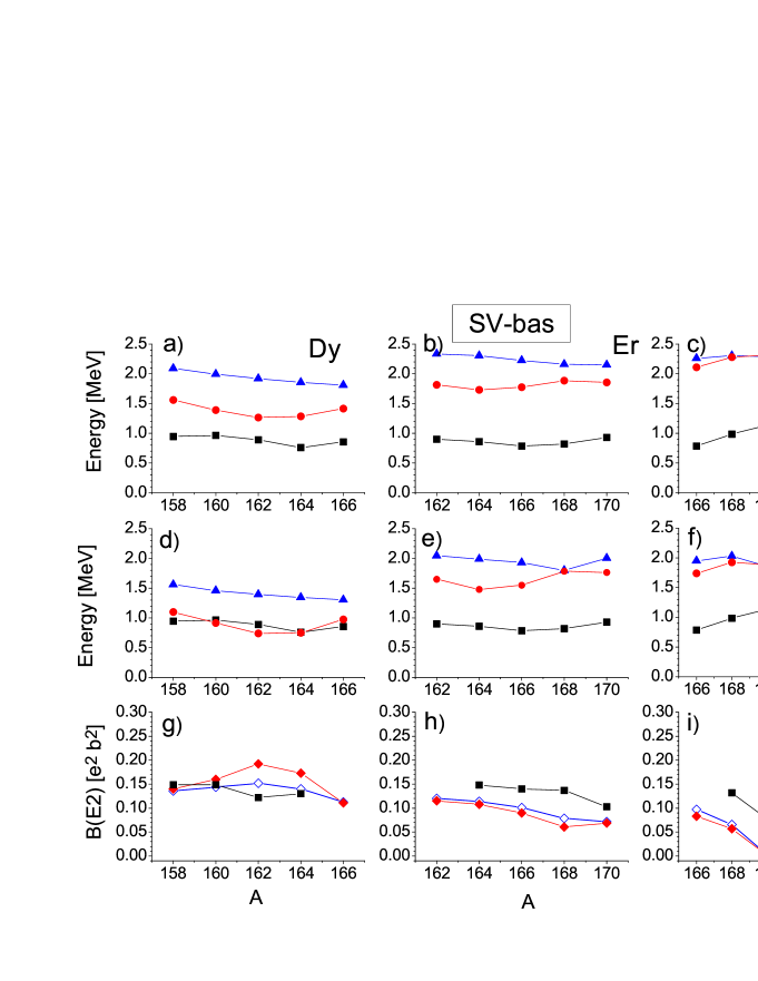
Figure 7: (Color online) The SV-bas results like in Fig. 5 but for Dy, Er, and Yb isotopes.

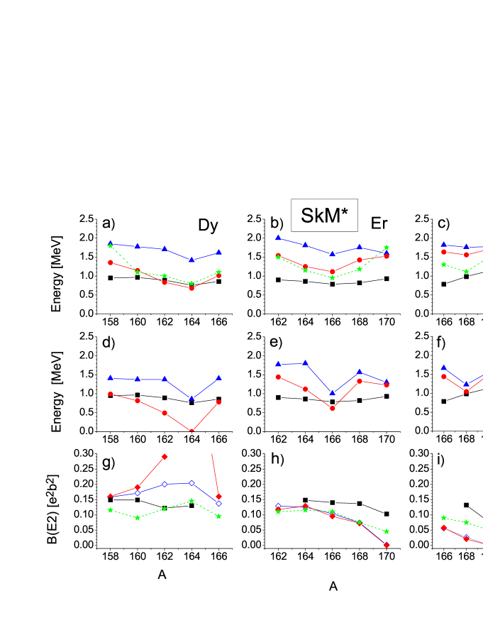
Figure 8: (Color online) The same as in Fig. 6 but for SkM^∗. At the plot g), the B(E2)=0.7 e²b² for ¹⁶⁴Dy is beyond the exhibited interval.

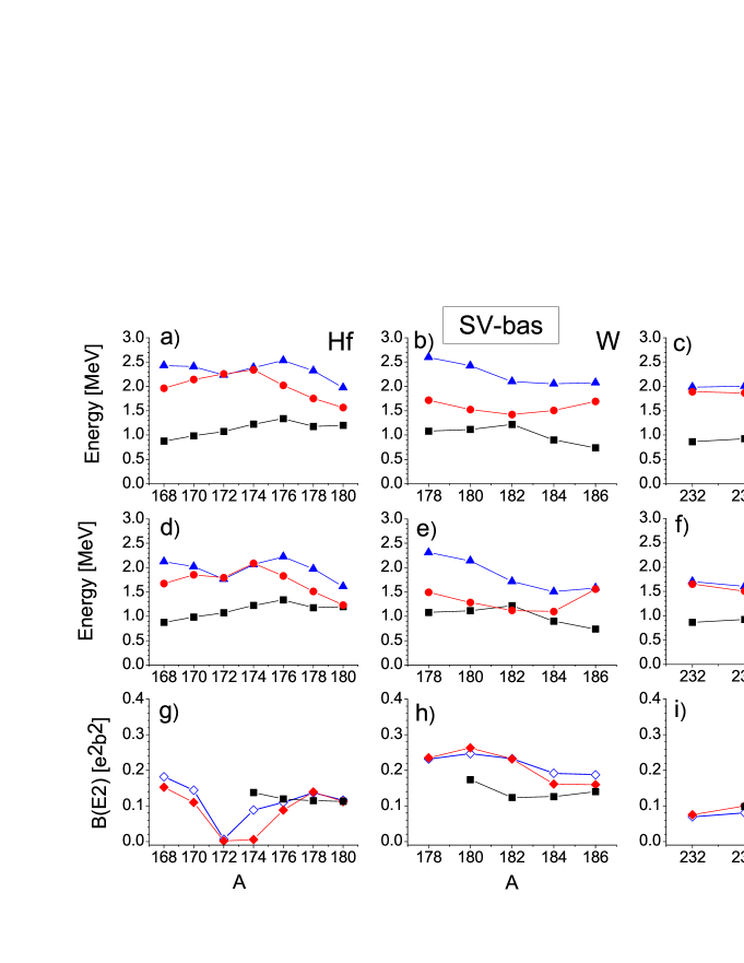
Figure 9: (Color online) The SV-bas results like in Fig. 7 but for Hf, W, and U isotopes.

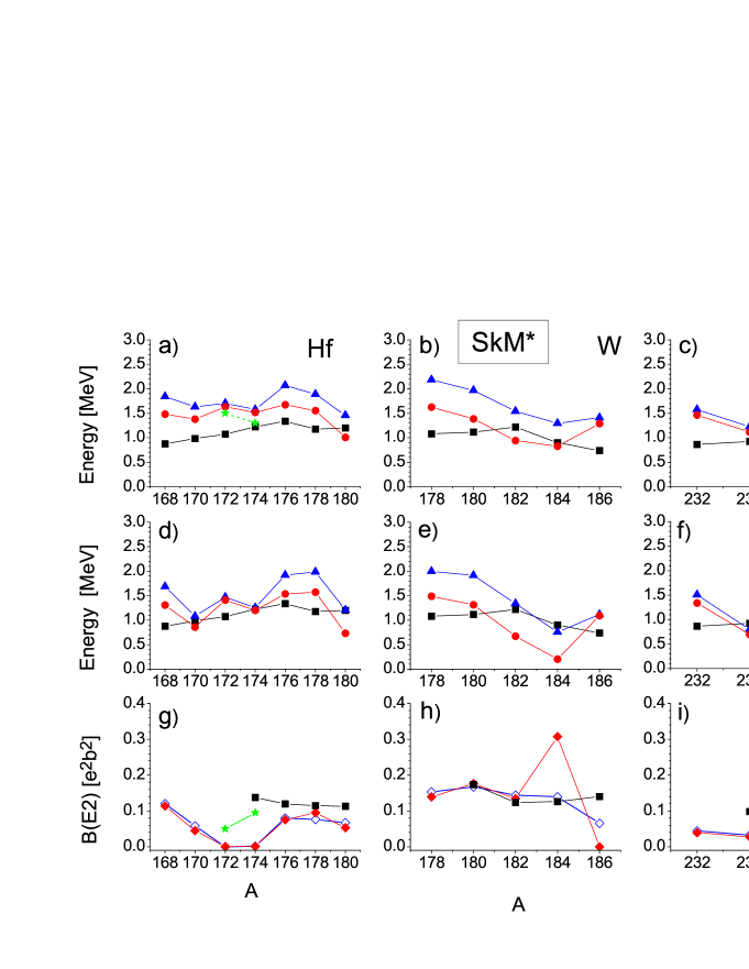
Figure 10: (Color online) The same as in Fig. 6 but for the force SkM^∗.

Fig. 5 shows the results for Nd, Sm and Gd isotopes obtained with SV-bas. Calculations without PBE (plots a-c) essentially overestimate the $2^{+}_{\gamma}$-energies. The discrepancy decreases from Nd to Gd with the growth of the collective shift $\Delta E=\mathcal{E}_{\rm{2qp}}-E_{\rm{SRPA}}$ (the difference between the lowest 2qp and SRPA energies). Accounting for the PBE noticeably downshifts the 2qp energies and thus the QRPA energies (plots d-f). The downshift reaches 0.1-0.6 MeV, depending on the isotope. As a result, the agreement with experimental energies improves, especially in heavy Gd isotopes. The trends of $E_{\rm{SRPA}}$ with mass number A are approximately reproduced. The B(E2) values in Sm and Gd with and without blocking are about the same. In Nd isotopes, the calculated $2^{+}_{\gamma}$ states demonstrate a weak collectivity, i.e. low B(E2) values. Here the PBE worsens the agreement. The SkM^∗ results in Fig. 6 for the same isotopes provide a similar quality of description. SRPA calculations without PBE well agree with HFB-QRPA ones Terasaki_PRC_11 , which indicates again the accuracy of SRPA.

Fig. 7 shows the SV-bas results for Dy, Er, and Yb isotopes. The collectivity of calculated $2^{+}_{\gamma}$ states reaches a maximum in Dy and Er isotopes. Here we have the largest $\Delta E$ and B(E2). The collectivity starts to decrease in heavy Er isotopes and almost vanishes in Yb. The PBE considerable decreases the 2qp and SRPA energies. In Dy isotopes, this leads to a nice agreement with the experimental energies and B(E2). In Er and Yb, the PBE noticeably improves the description of $2^{+}_{\gamma}$ energies. However $E_{\rm{RPA}}$ still remain considerably higher than $E_{\rm{exp}}$ and calculated B(E2) are accordingly underestimated.

The SkM^∗ results for Dy-Er-Yb isotopes are given in Fig. 8. We again observe a decrease of collectivity of $2^{+}_{\gamma}$ states from Dy to Yb isotopes. However, unlike the case of light rare-earth nuclei in Figs. 5-6, we also see a significant difference in the results of SV-bas and SkM^∗. First, as compared to SV-bas results and experimental data, the SkM^∗ energies in Er and Yb isotopes strongly fluctuate with A, closely following variations of 2p energies (this feature of SkM^∗ results was also mentioned in Terasaki_PRC_11 ). Such fluctuations point to a small collectivity of $2^{+}_{\gamma}$ states and significant contribution of the lowest 2qp state to the structure of $2^{+}_{\gamma}$ state. Furthermore, the 2qp energies are generally smaller for SkM^∗ than for SV-bas, which results in a better average description of $E_{\rm{exp}}$ in Er and Yb with SkM^∗. The PBE gives here larger changes than for Nd-Sm-Gd isotopes. In particular, it leads to a huge decrease of $2^{+}_{\gamma}$-energy in ¹⁶⁴Dy (like in Terasaki_PRC_11 ). This state becomes extremely collective (see a huge overestimation of experimental B(E2)). It is unlikely that it can be described within a familiar QRPA and needs a more involved prescription taking into account large ground state correlations Hara_gsc ; Vor_gsc ; Klu08 . The SRPA results agree with HFB-QRPA ones Terasaki_PRC_11 for Er-Yb but not for Dy, especially in the exceptional case of ¹⁶⁴Dy.

Figs. 9-10 show the results for heavy rare-earth Hf-W and actinide U isotopes. For both forces, the collectivity of $2^{+}_{\gamma}$ states increases from Hf to W and decreases in U. Moreover, both forces give rather similar trends of $E_{\rm{SRPA}}$ with A, though deviating from the experimental ones. The PBE considerably downshifts the 2qp and SRPA energies and thus in general improves their description. In average, SkM^∗ energies are closer to $E_{\rm{exp}}$ than SV-bas ones but give more fuzzy A-dependence, especially with PBE. In U isotopes, the description of the spectra with SkM^∗ is much better than with SV-bas, which again is explained by lower 2qp energies in SkM^∗. The description of B(E2) is acceptable in heavy Hf isotopes for both SV-bas and SkM^∗. With exception of ¹⁸⁴W, the PBE does not affect the description of B(E2).

Altogether, the results From Figs. 5-10 allow to do the following conclusions: i) In rare-earth and actinide regions, there are pronounced isotopic domains with low and high collectivity of $2^{+}_{\gamma}$ states. ii) The best agreement with the experimental data is obtained for Dy (except for ¹⁶⁴Dy) and W isotopes, i.e. for the most collective $2^{+}_{\gamma}$ states characterized by large $\Delta E$ and B(E2) values. iii) The PBE essentially downshifts 2qp and QRPA energies, thus leading to a better agreement with experiment. The value of the downshift is comparable with the collective shift $\Delta$E of QRPA and much larger than the experimental errors bnl_exp . This indicates that the PBE plays a non-negligible role for energies of low lying states. At the same time, the blocking also can have a small effect on the B(E2) values. Note that the results iii) should be checked within a truly self-consistent PBE-QRPA approach yet to be developed.

The above conclusions are supported by both SV-bas and SkM^∗. These two forces give similar results in light rare-earth nuclei but deviate in heavier nuclei. In SV-bas, the $E_{\rm{SRPA}}$ vary less with system size $A$ but are usually larger than $E_{\rm{exp}}$. In SkM^∗, the variation of $E_{\rm{SRPA}}$ is stronger but this force gives lower 2qp and SRPA energies and thus better describes $E_{\rm{exp}}$, e.g. in U isotopes. The differences are partly caused by a weaker pairing in SkM^∗ (the gaps in SkM^∗ are in average 30-50$\%$ smaller than in SV-bas). The latter in turn can follow from different level densities of SV-bas and SkM^∗ s-p spectra.

It is also useful to inspect the r.m.s. deviations of the calculated results from the experimental data,

$$\sigma_{b}=\sqrt{\frac{\sum_{i=1}^{\mathcal{N}_{b}}(b^{\rm{cal}}_{i}-b^{\rm{exp}}_{i})^{2}}{\mathcal{N}_{b}}},$$ (15)

where $b^{\rm{cal}}_{i}$ and $b^{\rm{exp}}_{i}$ are calculated and experimental values, $\mathcal{N}_{b}$ is the number of involved nuclei. The deviations for the QRPA energies ($\sigma_{E}$) and B(E2)-values ($\sigma_{B}$) are presented in Table 1. The cases with and without PBE are estimated. In the lower part of the Table, the SkM* SRPA deviations (without blocking) are compared with those of Ref. Terasaki_PRC_11 (manually obtained from the figures of Terasaki_PRC_11 ).

Table 1 confirms that inclusion of PBE significantly improves description of $2^{+}_{\gamma}$-energies but somewhat worsens reproduction of B(E2). This takes place for both SV-bas and SkM*. In agreement with previous findings, the SkM* noticeably better describes the energies than SV-bas. As compared to Terasaki_PRC_11 , SRPA demonstrates the better (similar) performance for $2^{+}_{\gamma}$-energies for the cases with (without) PBE. However SRPA results are generally worse for B(E2). Perhaps the latter is caused by the impact of the pp-channel which is included in Terasaki_PRC_11 but skipped in SRPA.

Following Table 1, the performance of both SRPA and HFB+QRPA Terasaki_PRC_11 is generally not good. The deviations $\sigma_{E,B}$ are large. This calls for further improvement of the description, e.g. for inclusion of the coupling to complex configurations (CCC). The calculated QRPA energies of $2^{+}_{\gamma}$ states mostly overestimate the experimental values. Thus we still have a window for CCC which, being a sort of additional correlations, can in some cases downshift the energies of the lowest excited states.

Table 1: Deviations between the calculated and experimental values of $2^{+}_{\gamma}$-energies ($\sigma_{E}$)and B(E2)-strengths ($\sigma_{B}$). $\mathcal{N}_{E,B}$ is the number of the involved nuclei. The SRPA deviations are compared with ones from Terasaki_PRC_11 .

	Skyrme	$\mathcal{N}_{E}$	$\sigma_{E}$ [MeV]		$\mathcal{N}_{B}$	$\sigma_{B}[e^{2}b^{2}]$
	force		no PBE	PBE		no PBE	PBE
	SV-bas	40	0.87	0.62	31	0.046	0.056
SRPA	SkM*	40	0.52	0.40∗)	31	0.059	0.075∗)
	SkM*	24	0.52	0.44∗)	18	0.061	0.072∗)
Ref.Terasaki_PRC_11	SkM*	24	0.49		18	0.034

^∗) In SkM* SRPA(PBE) estimation for $\sigma_{\scriptsize{E,B}}$, the anomalous nucleus ¹⁶⁴Dy is omitted ($\mathcal{N}_{E}$=39(23) and $\mathcal{N}_{B}$=30(17)).

Note also that the description of $2^{+}_{\gamma}$ states depends on a fragile balance of many factors (optimal s-p scheme, deformation, pairing with PBE and pp-channel, CCC with the corrections from the Pauli principle, etc) with comparable impacts. Moreover, these ingredients have opposite effects which partly compensate each other (e.g. the corrections from the Pauli principle may suppress the impact of CCC Sol_Shir ). Then, adding one of the factors, while ignoring its balance by others, may even worsen the description. In this connection, it would be premature to state, for example, that the performance of SV-bas for $2^{+}_{\gamma}$ states is worse than of SkM*. Also it would be wrong to state that if the effect of the particular factor is comparable with the dependence on the Skyrme parametrization, then this factor should be skipped. The final conclusions can be done only after collecting all the relevant factors which can affect the result.

Table 2: Features of the lowest (after blocking) 2qp (i,j) and corresponding $\lambda\mu\nu=221$ QRPA states in rare-earth nuclei, calculated with SV-bas and SkM^∗ forces. The table includes: the notation $qq[Nn_{z}\Lambda]_{i}[Nn_{z}\Lambda]_{j}$ of 2qp state in Nilsson quantum numbers; location of the s-p levels $i$ and $j$ relative to the Fermi (F) level; the quadrupole 2qp matrix element $f^{22}_{ij}=\langle ij|r^{2}Y_{22}|0\rangle$; the 2qp energy $\epsilon^{q}_{ij}$ (5) and collective shift $\Delta E=\epsilon^{q}_{ij}-E_{221}$, calculated without the blocking; the 2qp energy $\mathcal{E}^{q}_{\rm{bl}}(ij)$ (12) and collective shift $\Delta E_{\rm{bl}}=\mathcal{E}^{q}_{\rm{bl}}(ij)-E_{221}$, calculated with the blocking; the blocking correction $\Delta\mathcal{E}^{q}_{\rm{bl}}=\epsilon^{q}_{ij}-\mathcal{E}^{q}_{\rm{bl}}(ij)$. See text for more detail.

Nucleus	Force	$qq[Nn_{z}\Lambda]_{i}[Nn_{z}\Lambda]_{j}$	F-location	$f^{22}_{ij}$	$\epsilon^{q}_{ij}$	$\Delta E$	$\mathcal{E}^{q}_{\rm{bl}}(ij)$	$\Delta E_{\rm{bl}}$	$\Delta\mathcal{E}^{q}_{\rm{bl}}$
				[fm4]	[MeV]	[MeV]	[MeV]	[MeV]	[MeV]
${}^{154}_{\;\;62}$Sm92	SV-bas	pp[413]$\downarrow$[411]$\downarrow$	F, F+3	-4.43	2.57	0.46	2.34	0.38	0.23
	SkM∗	pp[411]$\downarrow$[411]$\uparrow$	F+3, F+1	4.98	2.45	0.34	2.37	0.31	0.07
${}^{162}_{\;\;66}$Dy96	SV-bas	pp[411]$\downarrow$[411]$\uparrow$	F+1, F	6.58	1.92	0.65	1.39	0.65	0.53
	SkM∗	pp[413]$\downarrow$[411]$\downarrow$	F, F+1	-5.78	1.71	0.87	1.37	0.88	0.33
${}^{164}_{\;\;66}$Dy98	SV-bas	pp[411]$\downarrow$[411]$\uparrow$	F+1, F	6.59	1.86	0.57	1.34	0.59	0.51
	SkM∗	nn[523]$\downarrow$[521]$\downarrow$	F, F+1	5.98	1.42	0.56	0.86	0.86	0.56
${}^{172}_{\;\;70}$Yb102	SV-bas	nn[512]$\uparrow$[521]$\downarrow$	F+1, F-1	0.37	2.40	0.003	2.12	-0.02	0.28
	SkM∗	nn[512]$\uparrow$[521]$\downarrow$	F+1, F-1	0.086	1.63	0.06	1.30	0.06	0.33
${}^{174}_{\;\;72}$Hf102	SV-bas	nn[512]$\uparrow$[521]$\downarrow$	F+1, F-1	0.37	2.39	-0.02	2.07	0.05	0.32
	SkM∗	nn[512]$\uparrow$[521]$\downarrow$	F+1, F-1	0.19	1.58	0.06	1.26	0.06	0.33
${}^{176}_{\;\;72}$Hf104	SV-bas	nn[512]$\uparrow$[510]$\uparrow$	F, F-2	-8.17	2.48	0.47	2.14	0.34	0.33
	SkM∗	nn[512]$\uparrow$[510]$\uparrow$	F, F-2	-8.48	2.53	0.51	2.23	0.39	0.31
${}^{182}_{\;\;74}$W108	SV-bas	nn[510]$\uparrow$[512]$\downarrow$	F+1, F+2	8.82	2.10	0.68	1.72	0.59	0.39
	SkM∗	nn[510]$\uparrow$[512]$\downarrow$	F+1, F+2	7.98	1.54	0.60	1.34	0.67	0.21

III.2 Discussion

In this subsection, we analyze the above results and compare them with earlier studies Terasaki_PRC_11 ; Sol_Grig ; Sol_Shir ; Sol_Sush_Shir .

First of all, it is worth to explore the origin of domains with low and high collectivity of $2^{+}_{\gamma}$ states. The low-collectivity domains include most of Nd, Er, Yb, Hf, and U isotopes. High collectivity exists in Sm, Gd, Dy, and W isotopes. Table 2 shows that the appearance of such domains is determined by the structure of the first 2qp states which, in turn, results in different absolute values of the matrix element $f^{22}_{ij}=\langle ij|r^{2}Y_{22}|0\rangle$ for the doorway operator $r^{2}Y_{22}$. These 2qp states are built from the levels close to the the Fermi level. High collectivity (pertinent to ¹⁵⁴Sm, ^162,164Dy, ¹⁷⁶Hf, and ¹⁸²W) takes place if the state is characterized by a large value of $|f^{22}_{ij}|$. Instead, if $|f^{22}_{ij}|$ is small, then we get non-collective $2^{+}_{\gamma}$ states (¹⁷²Yb and ¹⁷⁴Hf). The magnitude of $|f^{22}_{ij}|$ is determined by Nilsson selection rules for E2(K=2) transitions in axial nuclei Nilsson65 ; Sol76 . The rules read

$$\Delta K=2,\;\;\Delta N=0,\pm 2,\;\;\Delta n_{z}=0,\;\;\Delta\Lambda=2,$$ (16)

where $N$ is the principle quantum shell number, $n_{z}$ is the fraction of $N$ along the z-axis, $\Lambda$ is the orbital momentum projection onto z-axis. All the 2qp states in Table 2 fulfill the rules (16) for $K$ and $N$ but not for $n_{z}$ and $\Lambda$. Table 2 shows that the rule $\Delta n_{z}=0$ is decisive. The 2qp states which keep this rule (¹⁵⁴Sm, ^162,164Dy, ¹⁷⁶Hf, ¹⁸²W) exhibit $|f^{22}_{ij}|$-values of one order of magnitude larger than states violating the rule (¹⁷²Yb and ¹⁷⁴Hf). This effect is especially spectacular for neighboring isotopes ¹⁷⁴Hf - ¹⁷⁶Hf. The rule $\Delta\Lambda=2$ is not so crucial. However, matrix elements are additionally increased if this rule is obeyed (¹⁷⁶Hf, ¹⁸²W).

Table 2 obviously suggests that just the strength $|f^{22}_{ij}|$ of the first 2qp state is decisive for the collectivity of the QRPA $2^{+}_{\gamma}$ state and formation of the domains with low and high collectivity. This finding can be corroborated within a simple two-pole model given in Appendix C. Following this model, the collectivity of the lowest QRPA states is mainly determined by the ratio between the strengths of the first ($\nu$ =1) and second ($\nu$ =2) 2qp states where the second state simulates a cumulative effect of all 2qp states with $\nu>$1. Depending on this ratio, different scenarios can take place: high-collective limit, intermediate case and low-collective limit. In the last case, the first QRPA energy can lie even a bit above the first 2qp state, which happens, e.g., in our calculations for Yb isotopes.

Altogether, we get a simple recipe for predicting the collectivity of the first QRPA state: it suffices to inspect the Nilsson selection rules (16) for the lowest 2qp state, first of all $\Delta n_{z}=0$. Note that, unlike s-p spectra, the s-p wave functions and thus the values $|f^{22}_{ij}|$ only slightly depend on the Skyrme parametrization Nest04 , which makes the proposed recipe quite reliable. As seen from Table 1, SV-bas and SkM^∗ sometimes give different lowest 2qp states. Nonetheless, the correlation between $\Delta n_{z}=0$ rule and collectivity of QRPA $2^{+}_{\gamma}$-states applies in all considered cases.

The nucleus ¹⁶⁴Dy computed with SkM^∗ shows a remarkable sequence of four strong ($|f^{22}_{ij}|$=5.8-9.2 fm⁴) 2qp states which are located with PBE at 0.86 - 1.96 MeV. The cumulative impact of these states delivers a dramatic effect: a break-down of RPA. Without PBE, these four 2qp states lie at a higher energy 1.42–2.15 MeV and do not lead to the instability. For comparison, SV-bas gives in ¹⁶⁴Dy only three strong ($|f^{22}_{ij}|$=5.4-6.6 fm⁴) 2qp states and they are located at a higher energy 1.35-1.65 MeV. This gives a collective $2^{+}_{\gamma}$-state still within QRPA. Altogether, this discussion shows that some QRPA results for low lying states can be quite sensitive to the Skyrme force.

Table 2 shows that the values of collective shifts $\Delta E$ (up to 0.9 MeV) and blocking induced shifts $\Delta\mathcal{E}_{\rm{bl}}$ (up to 0.6 MeV) are comparable. Thus the PBE has a non-negligible effect in the present calculations.

The results exhibited in Figs. 5-10 indicate that the present Skyrme QRPA description of $2^{+}_{\gamma}$ states is not yet fully satisfactory. Though we get rather good agreement with experimental data for collective $2^{+}_{\gamma}$ states in Gd, Dy, and W isotopes, collectivity is generally underestimated in other isotopic chains (which is seen from too high SRPA energies and sizable low B(E2)-values). Perhaps the latter cases require a coupling to complex configurations, which might affect both the $2^{+}_{\gamma}$-energies and $B(E2)$-values. In this respect, our calculations indicate regions where CCC is needed. In the previous Skyrme QRPA study Terasaki_PRC_11 , the need for CCC was also pointed out. In nuclei like ¹⁶⁴Dy, an approach taking into account large ground state correlations is necessary Hara_gsc ; Vor_gsc .

As seen in Figs. 5-10, the performances of our and previous Terasaki_PRC_11 systematic Skyrme QRPA calculations (without the PBE) are rather similar. Although these calculations exploit different prescriptions, HFB + exact QRPA in Terasaki_PRC_11 and BCS+PBE + separable QRPA in the present study, they provide a remarkably similar description of QRPA energies of $2^{+}_{\gamma}$ states. The results Terasaki_PRC_11 are somewhat better for B(E2)-values, though the difference is not crucial.

Since SRPA operates with the residual interaction in a separable form, it can be directly compared with schematic separable QRPA approaches, e.g. with QPM which is widely and successfully used in nuclear spectroscopy Sol76 . The QPM proposes some simple relations for the strength constants of the residual interaction which might be useful for a rough evaluation of the SRPA strength constants. This analysis is done in the Appendix C. It is shown that the mixed isoscalar-isovector interaction might be essential in Skyrme QRPA. If this interaction is not properly balanced, it can weaken a general isoscalar effect of the residual interaction and thus make $2^{+}_{\gamma}$ states less collective (which might be relevant for Nd, Yb, Hf, U isotopes).

IV Summary

We have performed a systematic study of the lowest $\gamma$-vibrational $K^{\pi}=2^{+}$ states in axially deformed even-even rare-earth and actinide nuclei within a self-consistent (except for the pairing part) separable random-phase-approximation (SRPA) Ne06 . Nine isotopic chains involving 41 nuclei were explored. The excitation energies and B(E2)-values of $2^{+}_{\gamma}$ states were computed and analyzed. The Skyrme forces SV-bas SV and SkM^∗ SkMs were used. The force SV-bas was chosen as providing a good description of ground state deformations and isoscalar giant quadrupole resonance (ISGQR). SkM^∗ was used as a force with the best performance in the previous systematic study of $2^{+}_{\gamma}$ states Terasaki_PRC_11 , performed within the exact (not factorized) Skyrme HFB+QRPA. The accuracy of SRPA was confirmed by comparison with calculations within exact BCS+QRPA repko and BCS+QRPA Terasaki_PRC_11 .

Our study undertakes some important steps which were not realized earlier Terasaki_PRC_11 . Some essential points concerning the pairing contribution, systematics of $2^{+}_{\gamma}$ states and explanation of the results were scrutinized.

First, we have investigated a possible impact of the pairing blocking effect (PBE) on the properties of $2^{+}_{\gamma}$ states. Thereby we use in ”ad hoc” manner from the PBE only the correction of 2qp energies while the 2qp wave functions remain the same as in the BCS ground state. This scheme has significant advantages: it incorporates the most essential energy correction from PBE but maintains, at the same time, the orthonormality of the 2qp configuration space which, in turn, allows to apply the standard QRPA solution scheme. This blocking scheme was applied to a few lowest two-quasiparticle (2qp) configurations whose corrected energies were then used in SRPA calculations. Within this scheme, the PBE significantly downshifts the SRPA energies of $2^{+}_{\gamma}$ states and thus improves agreement with the experimental spectra. At the same time, PBE rather slightly affects collectivity of the states, expressed in terms of collective shifts and transition probabilities B(E2). It is to be noted, that our present handling of the PBE is very preliminary and should be further checked in fully developed self-consistent QRPA with PBE. To the best of our knowledge, such methods are still absent. Then our study can be viewed as a first step which highlights the problem and calls for a further self-consistent exploration. Note also that the PBE-QRPA scheme is certainly not the only way to improve the description of $2^{+}_{\gamma}$ states. Various many-body techniques that go beyond the plain QRPA, first of all the coupling to complex configuration, can be decisive here.

As the next novel aspect of our study, we have singled out domains of nuclei with a low and high collectivity of $2^{+}_{\gamma}$ states. It was shown that collectivity is mostly determined by the structure of the lowest 2qp state constituting the first SRPA 2qp state. The effect was explained in terms of the Nilsson selection rule $\Delta n_{z}$=0, which delivers a simple recipe to predict the $2^{+}_{\gamma}$-collectivity without performing QRPA calculations. Some results and SRPA characteristics were compared with those from the schematic Quasiparticle-Phonon Model (QPM) Sol76 which was successfully used for a long time in nuclear spectroscopy.

It was found that the forces SV-bas and SkM^∗ perform similarly in the description of $2^{+}_{\gamma}$ states for light rare-earth nuclei but deviate in heavier nuclei. The latter is mainly explained by the fact that SkM^∗ delivers a weaker pairing gap and thus lower 2qp energies, than SV-bas. SV-bas delivers less fuzzy trends of energies and B(E2) values and well describes Dy isotopes but fails in U isotopes. SkM^∗ is better in U isotopes but its results fluctuate more with the mass number. Moreover, SV-bas has an important advantage over SkM^∗: it well describes quadrupole equilibrium deformations and energy centroids of ISGQR. Thus SV-bas allows to get a consistent description of $2^{+}_{\gamma}$ states and ISGQR.

In general our study shows that, despite all the progress, available fully or partly self-consistent QRPA schemes are still not accurate enough for a satisfactory description of $2^{+}_{\gamma}$ states throughout medium and heavy axially deformed nuclei. This holds for both our results and previous ones Terasaki_PRC_11 . Some essential factors should be still added or improved. The proper calculation scheme should fulfill at least the following requirements: a) accurate description of the s-p spectra and equilibrium deformation, b) treatment of pairing (BCS or HFB) with PBE, c) self-consistent residual QRPA interaction with both ph- and pp-channels and consistently incorporated PBE, d) simultaneous description of other quadrupole excitations (ISGQR), e) systematic description involving nuclei from various mass regions and domains with a low and high collectivity, f) the coupling to complex configuration (with the proper inclusion of the Pauli principle). Some of these points will be a subject of our next studies.

Appendix A Pairing cut-off weight and pairing matrix elements

To simulate the effect of a finite range pairing force, the pairing-active space for each isospin $q$ is limited by using a smooth energy-dependent cut-off (see e.g. BCS50 ; Bon85 )

$$f^{q}_{k}=\frac{1}{1+\rm{exp}[\frac{\tilde{e}^{q}_{k}-\lambda_{q}-\Delta E_{q}}{\eta_{q}}]}$$ (17)

in the sums in Eqs. (9), (10), (13), and (II.2). The cut-off parameters $\Delta E_{q}$ and $\eta_{q}=\Delta E_{q}/10$ are chosen self-adjusting to the actual level density in the vicinity of the Fermi energy, see Ben00 for details.

For the $\delta$-force pairing interaction (3), the anti-symmetrized pairing matrix elements read

$$V_{i\bar{i}j\bar{j}}^{(\rm{pair,q})} = \langle i\bar{i}|V^{q}_{\rm{pair}}({\mathbf{r}},{\mathbf{r}}^{\prime})|j\bar{j}\rangle_{q}$$

$$= \int d^{3}r\int d{\mathbf{r}}^{\prime}\>\Phi^{+}_{i}({\mathbf{r}})\Phi^{+}_{\bar{i}}({\mathbf{r}}^{\prime})\>V_{q}\;\delta({\mathbf{r}}-{\mathbf{r}}^{\prime})$$

$$\cdot[\Phi_{j}({\mathbf{r}})\Phi_{\bar{j}}({\mathbf{r}}^{\prime})-\Phi_{j}({\mathbf{r}}^{\prime})\Phi_{\bar{j}}({\mathbf{r}})]$$

$$= V_{q}\int d^{3}r[\left(\Phi^{+}_{i}(\mathbf{r})\cdot\Phi_{j}(\mathbf{r})\right)\>\left(\Phi^{+}_{\bar{i}}(\mathbf{r})\cdot\Phi_{\bar{j}}(\mathbf{r})\right)$$

$$-\left(\Phi^{+}_{i}(\mathbf{r})\cdot\Phi_{\bar{j}}(\mathbf{r})\right)\left(\Phi^{+}_{\bar{i}}(\mathbf{r})\cdot\Phi_{j}(\mathbf{r})\right)]$$

where

$$\Phi_{i}(\mathbf{r})=\left(\begin{array}[]{rl}R^{(+)}_{i}(\rho,z)\>\>e^{i(K_{i}-\frac{1}{2})\vartheta}\\ R^{(-)}_{i}(\rho,z)\>\>e^{i(K_{i}+\frac{1}{2})\vartheta}\end{array}\right),$$ (19)

$$\Phi_{\bar{i}}(\mathbf{r})=\left(\begin{array}[]{rl}-R^{(-)}_{i}(\rho,z)\>\>e^{-i(K_{i}+\frac{1}{2})\vartheta}\\ R^{(+)}_{i}(\rho,z)\>\>e^{-i(K_{i}-\frac{1}{2})\vartheta}\end{array}\right)$$ (20)

are spinor s-p. wave functions in cylindrical coordinates $(\rho,z,\vartheta)$ and $\left(\Phi^{+}_{i}({\mathbf{r}})\cdot\Phi_{j}({\mathbf{r}})\right)$ are scalar products. Denoting the first (Hartree) and second (exchange) terms in the last line of (A) as $V_{i\bar{i}j\bar{j}}^{(\rm{pair-H,q})}$ and $V_{i\bar{i}j\bar{j}}^{(\rm{pair-ex,q})}$, we obtain

$$V_{i\bar{i}j\bar{j}}^{(\rm{pair-H,q})}=2\pi\>V_{q}\int_{0}^{\infty}d\rho\>\int_{-\infty}^{\infty}dz\>\rho$$ (21)

$$\left[2R_{i}^{(+)}R_{j}^{(+)}R_{i}^{(-)}R_{j}^{(-)}+(R^{(-)}_{i}R^{(-)}_{j})^{2}+(R^{(+)}_{i}R^{(+)}_{j})^{2}\right]\;,$$

$$V_{i\bar{i}j\bar{j}}^{(\rm{pair-ex,q})}=2\pi\>V_{q}\int_{0}^{\infty}d\rho\>\int_{-\infty}^{\infty}dz\>\rho$$ (22)

$$\left[-2R_{i}^{(+)}R_{j}^{(-)}R_{i}^{(-)}R_{j}^{(+)}+(R^{(-)}_{i}R^{(-)}_{j})^{2}+(R^{(+)}_{i}R^{(+)}_{j})^{2}\right]$$

and finally

$$V_{i\bar{i}j\bar{j}}^{(\rm{pair,q})} = V_{i\bar{i}j\bar{j}}^{(\rm{pair-H,q})}+V_{i\bar{i}j\bar{j}}^{(\rm{pair-ex,q})}$$

$$= 2\pi\>V_{q}\int_{0}^{\infty}d\rho\>\int_{-\infty}^{\infty}dz\>\rho$$

$$\left[(R_{i}^{(+)})^{2}+(R_{i}^{(-)})^{2}]\;[(R_{j}^{(+)})^{2}+(R_{j}^{(-)})^{2}]\right]\;.$$

Appendix B Basic SRPA equations

The self-consistent derivation Ne06 ; Ne_ar05 yields the SRPA Hamiltonian

$$\hat{H}=\sum_{q}\hat{h}^{q}_{\mathrm{HF+BCS}}+\hat{V}_{\mathrm{res}}$$ (24)

where

$$\hat{h}^{q}_{\mathrm{HFB}}=\int d{\mathbf{r}}\sum_{\alpha,\alpha^{\prime}}\left[\frac{\delta E}{\delta J^{q}_{\alpha}({\mathbf{r}})}\hat{J}_{q}^{\alpha}({\mathbf{r}})\right]$$ (25)

is the mean field and pairing contribution and

$$\hat{V}_{\rm{res}} = \frac{1}{2}\sum_{qq^{\prime}}\sum_{m,m=1}^{M}[\kappa_{qm,q^{\prime}m^{\prime}}\hat{X}_{qm}\hat{X}_{q^{\prime}m^{\prime}}$$

$$+ \eta_{qm,q^{\prime}m^{\prime}}\hat{Y}_{qm}\hat{Y}_{q^{\prime}m^{\prime}}]$$

is the separable residual interaction with one-body operators

$$\hat{X}_{qm} = \sum_{q^{\prime}}\hat{X}^{q^{\prime}}_{qm}=i\sum_{q^{\prime}}\sum_{\alpha,\alpha^{\prime}}\int d{\mathbf{r}}$$

$$\left[\frac{\delta^{2}E}{\delta J^{q^{\prime}}_{\alpha^{\prime}}({\mathbf{r^{\prime}}})\delta J^{q}_{\alpha}({\mathbf{r})}}\right]\langle\left[\hat{P}_{qm},\hat{J}^{q}_{\alpha}(\mathbf{r})\right]\rangle\hat{J}^{q^{\prime}}_{\alpha^{\prime}}(\mathbf{r^{\prime}})\;,$$

$$\hat{Y}_{qm} = \sum_{q^{\prime}}\hat{Y}^{q^{\prime}}_{qm}=i\sum_{q^{\prime}}\sum_{\alpha,\alpha^{\prime}}\int d{\mathbf{r}}$$

$$\left[\frac{\delta^{2}E}{\delta J^{q^{\prime}}_{\alpha^{\prime}}({\mathbf{r^{\prime}}})\delta J^{q}_{\alpha}({\mathbf{r})}}\right]\langle\left[\hat{Q}_{qm},\hat{J}^{q}_{\alpha}(\mathbf{r})\right]\rangle\hat{J}^{q^{\prime}}_{\alpha^{\prime}}(\mathbf{r^{\prime}})$$

and inverse strength matrices

$$\kappa_{qmq^{\prime}m^{\prime}}^{-1} = -i\langle[\hat{P}_{qm},{\hat{X}}_{q^{\prime}m^{\prime}}]\rangle,$$ (29)

$$\eta_{qmq^{\prime}m^{\prime}}^{-1} = -i\langle[\hat{Q}_{qm},{\hat{Y}}_{q^{\prime}m^{\prime}}]\rangle\;.$$ (30)

Here $\alpha=\rho,\tau,\mathbf{J},\chi,\mathbf{j},\mathbf{s},\mathbf{T}$ enumerates densities $J^{q}_{\alpha}$ and their operators $\hat{J}^{q}_{\alpha}$ while $m$ marks time-even $\hat{Q}_{qm}$ and time-odd $\hat{P}_{qm}=i[\hat{H},\hat{Q}_{qm}]$ Hermitian input (doorway) operators. The number $M$ of separable terms in (B) is determined by the number of the input operators $\hat{Q}_{qm}$ chosen from physical arguments Ne06 ; Ne02 . Usually we have $M=$3–5. For then, the QRPA matrix has a low rank $4M$ and we have small computational expense even for heavy deformed nuclei.

The values $\langle\left[\hat{P}_{qm},\hat{J}^{q}_{\alpha}\right]\rangle$ from (B) and $\langle\left[\hat{Q}_{qm},\hat{J}^{q}_{\alpha}\right]\rangle$ from (B) do not vanish only for time-even and time-odd densities $\hat{J}^{q}_{\alpha}$, respectively. Then $\hat{X}_{k}$ is time-even (determined by time-even densities) while $\hat{Y}_{k}$ is time-odd (determined by time-odd densities). The SRPA residual interaction (B) includes contributions from variations of both time-odd and time-even densities.

Following (25), (B) and (B), $\hat{h}_{\mathrm{HF+BCS}}$ and $\hat{V}_{\mathrm{r}es}$ are determined by first and second functional derivatives of the given energy functional. The model is self-consistent for exception of the pairing part.

The operators $\hat{Q}_{qm}$ constitute the key input for SRPA Ne06 ; Ne02 . They are chosen from physical arguments, namely to produce doorway states for particular excitations. In present calculations, four operators are used. The first one, $\hat{Q}_{q1}({\mathbf{r}})=r^{2}Y_{22}(\theta)+\rm{h.c.}$, generates the quadrupole ($\lambda\mu$=22) mode of interest in the long-wave approximation ($Y_{22}(\theta)$ is the spherical harmonic). Usually, already one such operator (generator) is enough for a rough description of the spectrum. However the corresponding Tassie mode Ri80 ; Tassie is mainly of the surface character. So, to improve accuracy of the description, two other generators, $\hat{Q}_{q2}({\mathbf{r}})=r^{4}Y_{22}(\theta)+\rm{h.c.}$ and $\hat{Q}_{q3}({\mathbf{r}})=j_{2}(0.6r)Y_{22}(\theta)+\rm{h.c.}$ (with $j_{2}(0.6r)$ being the spherical Bessel function), are added. These generators result in $\hat{X}^{q^{\prime}}_{qm}({\mathbf{r}})$ operators peaked more in the nuclear interior Ne06 . Finally, the generator $\hat{Q}_{q4}({\mathbf{r}})=r^{4}Y_{42}(\theta)+\rm{h.c.}$ is added to take into account the coupling between quadrupole and hexadecapole excitations in axially deformed nuclei. Note that these input operators do not form directly the separable residual interaction (B) but generate its operators $\hat{X}^{q^{\prime}}_{qm}({\mathbf{r}})$, $\hat{Y}^{q^{\prime}}_{qm}({\mathbf{r}})$ and strength constants $\kappa_{qm,q^{\prime}m^{\prime}}$, $\eta_{qm,q^{\prime}m^{\prime}}$, based on the initial Skyrme functional. The number $M$ of input operators determines the number of the separable terms in (B). Larger $M$ brings the separable interaction closer to the true (not factorized) one, but makes SRPA calculations more time consuming. The four operators which we are using here constitute a good compromise between reliability and expense.

SRPA allows to calculate the energies $\omega_{\nu}$ and wave function (with forward $\psi^{\nu}_{ij}$ and backward $\phi^{\nu}_{ij}$ 2qp amplitudes) of one-phonon $\nu$-states. Besides, various strength functions can be directly computed (without calculation of $\nu$-states). In this study, we use for description of ISGQR the strength function

$$S\>_{\gamma}(E22,\;E)=\sum_{\nu}\>|\>\langle\nu|\>r^{2}Y_{22}\>|0\rangle\>|^{2}\>\xi_{\Delta}(E-E_{\nu})$$ (31)

where $\xi_{\Delta}(E-E_{\nu})=\Delta/[2\pi((E-E_{\nu})^{2}+(\Delta/2)^{2}]$ is the Lorentz weight with the averaging parameter $\Delta$= 1 MeV.

The energy centroids for ISGQR depicted in Fig. 3 are estimated for the energy intervals where the strength functions exceeds 20$\%$ of its maximal value.

Appendix C Simple two-pole RPA model

Let’s consider SRPA with one input (doorway) operator and without time-odd contributions. Then the SRPA secular equation is reduced to the familiar equation for the schematic separable RPA Sol76 ; Ri80 :

$$\kappa^{-1}=\sum_{ij}\frac{f_{ij}^{2}}{\epsilon_{ij}^{2}-E_{\nu}^{2}}$$ (32)

where $\kappa$ is the strength constant, $f_{ij}$ is the matrix element of the residual interaction (including the pairing factors) between the states $i$ and $j$, $\epsilon_{ij}$ is the 2qp energy, and $E_{\nu}$ is the energy of the $\nu$-th RPA states. This equation may be simplified to the case of two 2qp states, yielding two poles in the schematic RPA equation:

$$1=\kappa f^{2}[\frac{k^{2}}{\epsilon^{2}_{1}-E^{2}}+\frac{1}{\epsilon^{2}_{2}-E^{2}}].$$ (33)

Here the first pole is characterized by the 2qp energy $\epsilon_{1}$ and matrix element $kf$. The second pole (with the 2qp energy $\epsilon_{2}>\epsilon_{1}$ and matrix element $f$) is assumed to simulate the effect of all the poles above the lowest one. The coefficient $k$ determines the ratio between the matrix elements of the first and second poles. We suppose $\kappa>0$, which is common for low-energy isoscalar excitations Sol76 .

Equation (33) is reduced to a standard quadratic equation

$$E^{4}+bE^{2}+c=0$$ (34)

with

$$b = -(\epsilon_{1}^{2}+\epsilon_{2}^{2})+\kappa f^{2}(1+k^{2}),$$ (35)

$$c = \epsilon_{1}^{2}\epsilon_{2}^{2}-\kappa f^{2}(\epsilon_{1}^{2}+k^{2}\epsilon_{2}^{2}).$$ (36)

This equation allows to get useful analytical estimations for three important cases: i) $k\gg 1$ (strong first pole, typical for Gd, Dy, and W isotopes), ii) $k\ll 1$ (weak first pole, typical for Nd, Yb, Hf, and U isotopes), iii) $k=1$ (intermediate case with equal strengths of the first and second poles).

We go through these three cases step by step:

i) For the strong first pole ($k\gg 1$), we get $(1\pm k^{2})\to\pm k^{2}$ and so

$$E^{2}\approx\frac{1}{2}[\epsilon_{1}^{2}+\epsilon_{2}^{2}-\kappa(fk)^{2}\pm(\epsilon_{1}^{2}-\epsilon_{2}^{2}-\kappa(fk)^{2})]$$ (37)

with two solutions

$$E^{2}_{+}\approx\epsilon^{2}_{1}-\kappa(fk)^{2},\;\;\;E^{2}_{-}\approx\epsilon^{2}_{2}$$ (38)

The solution $E_{+}$ gives the energy of the 1st RPA state below the first pole which is a common case in phenomenological QPM Sol76 ; Sol_Grig ; Sol_Shir . In our calculations, this case is met in Gd, Dy, and W isotopes.

ii) For the weak first pole ($k\ll 1$), we get $(1\pm k^{2})\to 1$ and so

$$E^{2} \approx \frac{1}{2}[\epsilon_{1}^{2}+\epsilon_{2}^{2}-\kappa f^{2}\pm(\epsilon_{1}^{2}-\epsilon_{2}^{2}+\kappa f^{2})],$$ (39)

$$E^{2}_{+} \approx \epsilon^{2}_{1},\;\;\;E^{2}_{-}\approx\epsilon^{2}_{2}-\kappa f^{2}.$$ (40)

The solution $E_{+}$ is the energy of the 1st RPA state close to the first pole. This energy can be both a bit smaller or larger than $e_{1}$. We have this case for Nd, Yb and Hf isotopes.

iii) If the pole strengths are equal ($k=1$), then $(1-k^{2})\to 0,\;(1+k^{2})\to 2$ and

$$E^{2}\approx\frac{1}{2}[\epsilon_{1}^{2}+\epsilon_{2}^{2}-2\kappa f^{2}\pm\sqrt{(\epsilon_{1}^{2}-\epsilon_{2}^{2})^{2}+4\kappa^{2}f^{4}}.$$ (41)

Supposing that $(\epsilon_{1}^{2}-\epsilon_{2}^{2})^{2}\gg 4\kappa^{2}f^{4}$, we get

$$E^{2} \approx \frac{1}{2}[\epsilon_{1}^{2}+\epsilon_{2}^{2}-2\kappa f^{2}\pm(\epsilon_{1}^{2}-\epsilon_{2}^{2}+\kappa f^{2})],$$ (42)

$$E^{2}_{+} \approx \epsilon^{2}_{1}-\frac{1}{2}\kappa f^{2},\;\;\;E^{2}_{-}\approx\epsilon^{2}_{2}-\frac{3}{2}\kappa f^{2}.$$ (43)

This simple model indicates that collectivity (collective shift $\Delta E=E_{+}-\epsilon_{1}$) of the first RPA state is determined to a large extent by the relative strength of the first pole. This conclusion is confirmed by our numerical results, see discussion of Table 2. Thus we have found a simple way for the prediction of the collectivity (weak or large) of the first RPA state. In practice, it is enough to compare the matrix elements of the first and next poles. Or, which is even easier, one should check if the first pole fulfills the $\Delta n_{z}$=0 Nilsson selection rule.

Appendix D Comparison with QPM

Since SRPA deals with a separable residual interaction, this method can be directly compared with the schematic separable QRPA exploited in QPM Sol76 . The QPM is not self-consistent: it uses the Woods-Saxon s-p basis and its isoscalar $\kappa_{00}$ and isovector $\kappa_{11}$ strength constants of the residual interaction are adjusted to reproduce the experimental energies of lowest vibrational states and giant resonances. However, just because of the successful combination of the microscopic and phenomenological aspects, the QPM is known to be quite accurate in description of low-energy states. Thus it is instructive to compare the characteristics of self-consistent models, like Skyrme QRPA, with the relevant QPM parameters.

In this connection, let’s briefly discuss the QPM strength constants of the residual interaction and compare them with the SRPA ones. The strength constants in the proton-neutron domain (nn, pp, np) can be related to their counterparts in the isoscalar-isovector domain (00,11, 01) as

$$\kappa_{00} =\frac{1}{2}( \kappa_{pp}+\kappa_{pn}+\kappa_{np}+\kappa_{nn}),$$ (44)

$$\kappa_{11} =\frac{1}{2}( \kappa_{pp}-\kappa_{pn}-\kappa_{np}+\kappa_{nn}),$$ (45)

$$\kappa_{01} =\frac{1}{2}( \kappa_{pp}-\kappa_{pn}+\kappa_{np}-\kappa_{nn})=\kappa_{10}.$$ (46)

The constants $\kappa_{01}=\kappa_{10}$ represent the mixing between isoscalar (00) and isovector (11) excitations. This mixing can be motivated by both physical (Coulomb interaction, etc) and technical (different sizes of neutron and proton s-p basis, etc) reasons. Since nuclei roughly keep the isospin symmetry, then

$$|\kappa_{00}|,|\kappa_{11}|\gg|\kappa_{01}=\kappa_{10}|.$$ (47)

If to assume $\kappa_{01}=\kappa_{10}=0$ and $\kappa_{np}=\kappa_{pn}$, then we get

$$\kappa_{pp}=\kappa_{nn}$$ (48)

and the familiar QPM relations Sol76

$$\kappa_{00}=\kappa_{pp}+\kappa_{pn},\qquad\kappa_{11}=\kappa_{pp}-\kappa_{pn}.$$ (49)

¿From (49) one gets

$$\kappa_{pp}=\kappa_{nn} = \frac{1}{2}(\kappa_{00}+\kappa_{11}),$$ (50)

$$\kappa_{pn}=\kappa_{np} = \frac{1}{2}(\kappa_{00}-\kappa_{11})$$ (51)

where $\kappa_{11}=\alpha\kappa_{00}$ with $\kappa_{00}>0$. Usually $\alpha$=-1.5 is used Sol_Shir , which results in a dominance of the np-interaction, $\kappa_{pn}/\kappa_{pp}$=-2.5 with $\kappa_{pn}=\kappa_{np}>0$ and $\kappa_{pp}=\kappa_{nn}<0$.

For the comparison, the self-consistent SRPA calculations give somewhat different picture. As a relevant example, the strength constants $\kappa_{q1,q^{\prime}1}=\kappa_{qq^{\prime}}$ for the dominant first input operator $r^{2}Y_{22}$ in ¹⁶²Dy are considered. Note that in SRPA the relation $\kappa_{pn}=\kappa_{np}$ is kept. SV-bas10 gives strength constants $\kappa_{pp},\kappa_{nn},\kappa_{pn}>0$ with the relations $\kappa_{pp}/\kappa_{nn}$=2.7, $\kappa_{pn}/\kappa_{pp}$=7.7 and $\kappa_{pn}/\kappa_{nn}$=2.9. Similar results are obtained in other nuclei. SkM^∗ gives $\kappa_{nn},\kappa_{pn}>0$, $\kappa_{pp}<0$ and relations $\kappa_{pp}/\kappa_{nn}$=-2.0, $\kappa_{pn}/\kappa_{pp}=-4.4$, and $\kappa_{pn}/\kappa_{nn}$= 2.2. In agreement with QPM, both forces provide a dominant np-interaction with the proper sign. However, in contrast to (48), the weak SRPA constants $\kappa_{pp}$ and $\kappa_{nn}$ noticeably deviate from each other, which might be a signature of an large mixing of the isoscalar and isovector interaction. Perhaps just this mixing, if not be properly balanced with other parts of the interaction, partly leads to the troubles of Skyrme QRPA with the description of $2^{+}_{\gamma}$ states. A difference in sign of SV-bas and SkM^∗ constants $\kappa_{pp}$ should be also mentioned as demonstration of the noticeable dependence of the residual interaction on the Skyrme force.

References

- (1) M. Bender, P.-H. Heenen, and P.-G. Reinhard, Rev. Mod. Phys. 75, 121 (2003).
- (2) D. Vretenar, A.V. Afanasjev, G.A. Lalazissis, P. Ring, Phys. Rep.409 101 (2005).
- (3) N. Paar, D. Vretenar, E. Khan, and G. Colo, Rep. Prog. Phys. 70, 691 (2007).
- (4) J. Erler, W. Kleinig, P. Klüpfel, J. Kvasil, V.O. Nesterenko, and P.-G. Reinhard, Phys. Part. Nucl. 41 851 (2010).
- (5) V.O. Nesterenko, W. Kleinig, J. Kvasil, P. Vesely, P.-G. Reinhard, and D.S. Dolci, Phys. Rev. C74, 064306 (2006).
- (6) K. Yoshida and N.V. Giai, Phys. Rev. C78, 064316 (2008).
- (7) D. Pena Arteaga and P. Ring, Phys. Rev. C77, 034317 (2008).
- (8) C. Losa, A. Pastore, T. Døssing, E. Vigezzi, and R. A. Broglia, Phys. Rev. C81, 064307 (2010).
- (9) J. Terasaki and J. Engel, Phys. Rev. C82, 034326 (2010).
- (10) J. Terasaki and J. Engel, Phys. Rev. C84, 014332 (2011).
- (11) S. Péru and H. Goutte, Phys. Rev. C77, 044313 (2008).
- (12) S. Péru, G.Gosselin, M. Martini, M. Dupuis, S. Hilaire, and J.-C. Devaux, Phys. Rev. C83, 014314 (2011).
- (13) T. Inakura, T. Nakatsukasa, and K. Yabana, Phys. Rev. C80, 044301 (2009).
- (14) S. Fracasso, E.B. Suckling, and P.D. Stevenson, Phys. Rev. C86, 044303 (2012).
- (15) N. Hinohara, M. Kortelainen, and W. Nazarewicz, Phys. Rev. C87, 064309 (2013).
- (16) V.O. Nesterenko, W. Kleinig, J. Kvasil, P. Vesely, and P.-G. Reinhard, Int. J. Mod. Phys. E, 17, 89 (2008).
- (17) W. Kleinig, V.O. Nesterenko, J. Kvasil, P.-G. Reinhard, and P. Vesely, Phys. Rev. C78, 044313 (2008).
- (18) J. Kvasil, V.O. Nesterenko, W. Kleinig, D. Bozik, P.-G. Reinhard, and N. Lo Iudice, Eur. Phys. J. A49, 119 (2013).
- (19) P. Vesely, J. Kvasil, V.O. Nesterenko, W. Kleinig, P.-G. Reinhard, and V.Yu. Ponomarev, Phys. Rev. C80, 031302(R) (2009).
- (20) Evaluated Nuclear Structure Data File [http://www.nndc.bnl.gov].
- (21) E.P. Grigorjev and V.G. Soloviev, Structure of even deformed nuclei, (Moscow, Nauka, 1974).
- (22) V.G. Soloviev, Theory of Atomic Nuclei, (Oxford, Pergamon Press, 1976).
- (23) V.G. Soloviev and N.Yu. Shirikova, Z. Phys. A - Atomic Nuclei 334, 149(1989).
- (24) V.G. Soloviev, A.V. Sushkov, and N.Yu. Shirikova, Part. Nucl. 27, n.6, 1643 (1996).
- (25) J. Bartel, P. Quentin, M. Brack, C. Guet, and H.-B. Haakansson, Nucl. Phys. A386, 79 (1982).
- (26) E. Chabanat, P. Bonche, P. Haensel, J. Meyer, and R. Schaeffer, Nucl. Phys. A635, 231 (1998).
- (27) P. Klupfel, P.-G. Reinhard, T.J. Burvenich, and J.A. Maruhn, Phys. Rev. C79, 034310 (2009).
- (28) V.O. Nesterenko, V. G. Kartavenko, W. Kleinig, R.V. Jolos, J. Kvasil, and P.-G. Reinhard, arXiv:1504.06492[nucl-th].
- (29) K. J. Pototzky, J. Erler, P.-G. Reinhard, and V. O. Nesterenko, Eur. Phys. J. A 46, 299 (2010).
- (30) J. M. Eisenberg, and W. Greiner, Nuclear Theory: Microscopic Theory of the Nucleus, Vol. III (North-Holland, Amsterdam, London, 1972).
- (31) P. Ring and P. Schuck, Nuclear Many Body Problem, (Springer-Verlag, New York, 1980).
- (32) S. G. Nilsson, and I. Ragnarsson, Shapes and Shells in Nuclear Structure, (Cambridge University Press, Cambridge, 1995).
- (33) Fifty Years of Nuclear BCS, ed. by R.A. Broglia and V. Zelevinsky (World Scientific, Singapure, 2013).
- (34) M. Bender, K. Rutz, P.-G. Reinhard, and J.A. Maruhn, Eur. Phys. J. A8, 59 (2000).
- (35) T.H.R. Skyrme, Phil. Mag. 1, 1043 (1956).
- (36) D. Vauterin, D.M. Brink, Phys. Rev. C5, 626 (1972).
- (37) V.O. Nesterenko, J. Kvasil, and P.-G. Reinhard, Phys. Rev. C66, 044307 (2002).
- (38) V.O. Nesterenko, J. Kvasil, W. Kleinig, P.-G. Reinhard, and D.S. Dolci, arXiv:nucl-th/0512045.
- (39) A. Repko, J. Kvasil, V.O. Nesterenko, and P.-G. Reinhard, arXiv:1510.01248[nucl-th].
- (40) S. Raman, C.W. Nestor, Jr., and P. Tikkanen, At. Data and Nucl. Data Tables, 78, 1 (2001).
- (41) P.G. Reinhard, private communication.
- (42) T. Duguet, P. Bonche, P.-H. Heenen, and J. Meyer, Phys. Rev. C65, 014310 (2001).
- (43) N.K. Kuzmenko, V.M. Mikhailov, and V.O. Nesterenko, Izv. Akad. Nauk, Ser. Fiz., 50, 1914 (1986).
- (44) J. Dobaczewski, M.V. Stoitsov, W. Nazarewicz, and P.-G. Reinhard, Phys. Rev. C 76, 054315 (2007).
- (45) G. Scamps and D. Lacroix, Phys. Rev. C88, 044310 (2013).
- (46) A.P. Severyukhin, V.V. Voronov, and N.V. Giai, Phys. Rev. C77, 024322 (2008).
- (47) S.G. Nilsson, Mat. Fys. Medd. Dan. Vid. Selsk. 29, n.16 (1965).
- (48) V.O. Nesterenko, V.P. Likhachev, P.-G. Reinhard, V.V. Pashkevich, W. Kleinig, and J. Mesa, Phys. Rev. C70, 057304 (2004).
- (49) K.E. Hara, Progr. Theor. Phys. 32, 88 (1964).
- (50) V.V. Voronov, D. Karadjov, F. Catara, and A.P. Severyukhin, Sov. J. Part. Nucl, 31, 905 (2000).
- (51) P. Klüpfel, J. Erler, P.-G. Reinhard, and J. A. Maruhn, Eur. Phys. J., A37, 343 (2008).
- (52) P. Bonche, H. Flocard, P.H. Heenen, S.J. Krieger, M.S. Weiss, Nucl. Phys. A443, (1985) 39.
- (53) L.J. Tassie, Austr. J. Phys. 9, 407 (1956).