I INTRODUCTION

The correct determination of the threshold energy of Quark Gluon Plasma formation (QGP) is one of the major goals of modern heavy ion physics. The experiments planned at FAIR Bleich11 and NICA Kolesnik13 are targeted to study the properties of exotic nuclear matter created in nucleus-nucleus (A+A) collisions and to figure out a precise position of the critical endpoint of the deconfinement phase transition Fukushim11 . The Beam Energy Scan program performed at RHIC revealed somewhat different properties of strongly interacting matter created in A+A collisions at energies below and above $\sqrt{s_{NN}}\,=\,11.5$ GeV Mohanty13 . At the same time, the experiments on central heavy ion collisions done at AGS and SPS found such remarkable irregularities as the Strangeness Horn in $K^{+}/\pi^{+}$ ratio at $\sqrt{s_{NN}}\,=\,7.6$ GeV Alt08 and the peaks of $\bar{\Lambda}/\bar{p}$ and $\Lambda/\pi^{-}$ ratios at energies about $\sqrt{s_{NN}}\,=\,5-6$ GeV Wang12 ; Alt008 . Although there exist some claims Horn ; Step ; Gazd_rev:10 that the Strangeness Horn signals about the onset of deconfinement, the convincing explanation of its relation to the deconfinement is, in fact, absent. Despite the fact that a very successful description of the $K^{+}/\pi^{+}$ and $\Lambda/\pi^{-}$ peaks is achieved recently in Bugaev13:Horn ; Bugaev13:SFO ; Sagun14:Lambda , such a success does not provide an apparent relation between the strangeness enhancement at these collision energies and the deconfinement transition.

Moreover, nowadays not only the situation with the “signals” of QGP formation is unclear, but also there is no consensus on its formation threshold energy. For example, the authors of Strangeness Horn “signal” Horn , claim that the onset of deconfinement starts at $\sqrt{s_{NN}}\,=\,7.6$ GeV Gazd_rev:10 . On the other hand, the authors of RafLet state that the onset of deconfinement occurs at $\sqrt{s_{NN}}\,=\,6.3$ GeV, while very recently there appeared the works Bugaev:2014a ; Bugaev:2014b which are arguing that the hadron-QGP mixed phase is formed at $\sqrt{s_{NN}}\,=\,4.2-4.9$ GeV. Regarding these threshold energy values, we would like to stress that the works Horn ; Step ; Gazd_rev:10 ; RafLet do not provide the underling statistical or hydrodynamic or microscopic models which are able to connect their “signals” with the very fact of the hadron-QGP mixed phase formation. In Refs. Bugaev:2014a ; Bugaev:2014b the underlying hydrodynamic model of phase transition which explains the observed irregularities is developed, but similarly to the works mentioned above, i.e. Gazd_rev:10 ; RafLet , the model of Refs. Bugaev:2014a ; Bugaev:2014b is also relying only on a certain set of experimental data from many sets of existing data.

At the same time various sets of experimental data (the transverse mass or transverse momentum distributions, the longitudinal rapidity distributions of several hadron species, the total or/and midrapidity yields of various hadrons e.t.c.) are, in principle, available and the results of a few event generators of A+A collisions are published. These generators can be divided into two major groups: the first group includes the QGP state in their description (QGP models), while the second group does not include the QGP formation, i.e. Hadron Gas (HG) models. If the existing generators of A+A collisions contain just a grain of truth, then, we believe, it is worth to systematically compare their ability to reproduce experimental data and to find out this grain from such a comparison. Hence, in this work we suggest to employ both the available sets of data and the theoretical models describing them in order to elucidate the correct value of the threshold energy of the hadron-QGP mixed phase.

Our main idea is based on the assumption that the HG models of A+A collisions should provide worse description of the data above the QGP threshold energy, whereas below this threshold they should be able to better (or at least not worse) reproduce data compared to the QGP models. Furthermore, we assume that both kinds of models should provide an equal and rather good QDD at the energy of mixed phase production. Hence, the mixed phase production threshold should be slightly below the energy at which the equal QDD is changed to the essential worsening of QDD by HG models.

The second primary aim of this work is to make a comparative study of two classes of the event generators of A+A collisions. This is necessary to fix the present days status quo, to make a realistic plan of further experiments on A+A collisions and to formulate the most important tasks for theoretical studies.

The work is organized as follows. In the next section we present the basic elements of our meta-analysis. Section III is devoted to a detailed description of two ways of averaging used in this meta-analysis on the example of the data sets available at $\sqrt{s_{NN}}\,=$ 4.87 GeV. The results and their interpretation are given in section IV, while section V contains our conclusions and practical suggestions for planning experiments.

II ANALYSIS OF DATA AND MODELS

As it was discussed above, the existing approaches Gazd_rev:10 ; RafLet suggest that the onset of deconfinement begins somewhere between the highest AGS and the lowest SPS energies, i.e. in the collision energy range $\sqrt{s_{NN}}\,=$ 4.2 GeV Bugaev:2014a ; Bugaev:2014b – 7.6 GeV Horn ; Step ; Gazd_rev:10 . The main reason for such a range is that almost all irregularities observed either at kinetic freeze-out Horn ; Step ; Gazd_rev:10 or at chemical freeze-out RafLet ; Bugaev:2014a ; Bugaev:2014b ; Bugaev:2013irr belong to this energy range. Therefore, to compare the QGP and HG models we choose the AGS data measured in Au+Au collisions at $\sqrt{s_{NN}}\,=$ 3.1 GeV as the lower bound of collision energy. On the other hand, we extended the upper bound of collision energy from $\sqrt{s_{NN}}\,=$ 7.6 GeV to $\sqrt{s_{NN}}\,=$17.3 GeV, since there are arguments Quarkyonic that at $\sqrt{s_{NN}}\,\simeq$ 10 GeV there may exist the tricritical endpoint of the strongly interacting matter phase diagram, which in Quarkyonic is mistakenly called a triple point. Hence, we will be able to investigate the wider energy range than the most interesting one.

Our choice of collision energies $\sqrt{s_{NN}}\,=$ 3.1, 3.6, 4.2, 4.87, 5.4, 6.3, 7.6, 8.8, 12.3 and 17.3 GeV is also dictated by the fact that exactly for these energies there were multiple efforts to describe the experimental data both by the QGP and by the HG generators. Therefore, in the chosen collision energy range a comparison of the QDD provided by these two types of models can be made in details. The collision energies $\sqrt{s_{NN}}\,\leq$ 4.87 GeV correspond to Au+Au reactions studied at AGS. At $\sqrt{s_{NN}}\,=$ 5.4 GeV the reactions Pb+Si, Si+Si and Si+Al were also studied at AGS, while higher values of collision energy correspond to Pb+Pb reactions investigated at SPS.

The main object of our meta-analysis is the mean deviation squared of the quantity $A^{model,h}$ of the model M from the data $A^{data,h}$ per number of the data points $n_{d}$ for a given particle type $h$

$$\langle\chi^{2}/n\rangle^{h}_{A}\biggl{|}_{M}=\frac{1}{n_{d}}\sum\limits_{k=1}^{n_{d}}\left[\frac{A^{data,h}_{k}-A^{model,h}_{k}}{\delta A_{k}^{data,h}}\right]^{2}\biggl{|}_{M}\,,$$ (1)

where $\delta A_{k}^{data,h}$ is an experimental error of the experimental quantity $A^{data,h}_{k}$ and the summation in Eq. (1) runs over all data point at given collision energy. To get the most complete picture of the A+A collision process dynamics, we have to compare the available data on the transverse mass ($m_{T}$) distributions $A=\frac{1}{m_{T}}\,\frac{d^{2}N(m_{T},y)}{dm_{T}dy}$, the longitudinal rapidity ($y$) distributions $A=\frac{dN(y)}{dy}$ and the hadronic yields (Y) measured at midrapidity $A=\frac{dN(y=0)}{dy}$ or/and the total one, i.e. measured within 4$\pi$ solid angle, since right these observables are traditionally believed to be sensitive to the equation of state properties Shuryak .

Based on the theory of measurements Taylor82 , we consider the set of quantities $\langle\chi^{2}/n\rangle^{h}_{A}\biggl{|}_{M}$ as the results of the meta-measurements of the same meta-quantity, i.e. the QDD of $\{A^{data,h}_{k}\}$ data, with the different meta-devices, i.e. models $\{M\}$, with the hadronic probe $h$. The whole set of quantities $\langle\chi^{2}/n\rangle^{h}_{A}\biggl{|}_{M}$ allows one to find the mean value $\langle\chi^{2}/n\rangle_{M}$ properly averaged over the experimental data and over models belonging to the same class, i.e. M=HG or M=QGP, and over all hadronic species. Using the averaged values for two classes of models $\langle\chi^{2}/n\rangle_{HG}$ and $\langle\chi^{2}/n\rangle_{QGP}$, we could find the regions of their preferential and their comparable description of the experiments. The latter case could provide us with the most probable collision energy range of the hadron-QGP mixed phase threshold. Unfortunately, the published articles usually do not provide one with the quantities $\langle\chi^{2}/n\rangle^{h}_{A}\biggl{|}_{M}$. An exception is the article S4.9a , in which one can find the desired values for the $m_{T}$ spectra of $\Lambda$-hyperons for 4 rapidity intervals measured in Au+Au collisions at highest AGS energy. Therefore, using the modern software we calculated the set of quantities $\langle\chi^{2}/n\rangle^{h}_{A}\biggl{|}_{M}$ and their errors $\delta\langle\chi^{2}/n\rangle^{h}_{A}\biggl{|}_{M}$ from the published papers.

The theoretical models taken for the present analysis belong to two groups:

• The used HG models are as follows: ARC Arc , RQMD2.1(2.3) RQMD , HSD HSDgen ; S5.4a , UrQMD1.3(2.0, 2.1, 2.3) Bass98 , statistical hadronization model (SHM) SHMgen and AGSHIJET_N* HIJETa ; S5.4b . These models do not include the QGP formation in the process of A+A collisions. The results of the HG models were taken from the following publications: ARC S4.9a ; S5.4b , RQMD2.1(2.3) S4.9a ; S4.9b , HSD S5.4a ; S4.9KL , UrQMD1.3(2.0, 2.1, 2.3) S4.9KL ; Blume , SHM SHM ; Blume and AGSHIJET_N* S5.4b . Further details on what data at what energies were analyzed are presented in Tables I and III-XI.

• The used QGP models are as follows: Quark Combination (QuarkComb) model QComb , 3-fluid dynamics (3FD) model 3FDgen ; 3FDII ; 3FDIII , PHSD model PHSDgen ; Phsd and Core-Corona model CoreCorMa ; CoreCorMb . These generators explicitly assume the QGP formation in A+A collisions. The results of the QGP models were taken from the following publications: QuarkComb model QComb , 3FD model 3FDII ; 3FDIII , PHSD model Phsd and Core-Corona model CoreCor . More details on the analyzed data and energies can be found in Tables I and III-XI.

A short description of these models along with the criteria of their selection can be found in the Appendix.

Our meta-analysis requires the well-defined errors for the quantities $\langle\chi^{2}/n\rangle^{h}_{A}\biggl{|}_{M}$. They were defined according to the rule of indirect measurements Taylor82 as

$$\Delta_{A}\langle\chi^{2}/n\rangle^{h}_{A}\biggl{|}_{M} \equiv \left[\sum\limits_{k=1}^{n_{d}}\left[\delta A_{k}^{data,h}\,\frac{\partial\langle\chi^{2}/n\rangle^{h}_{A}\biggl{|}_{M}}{\partial~{}A^{data,h}_{k}}\right]^{2}\right]^{\frac{1}{2}}$$ (2)

$$= \frac{2}{n_{d}}\left[\sum\limits_{k=1}^{n_{d}}\left[\frac{A^{data,h}_{k}-A^{model,h}_{k}}{\delta A_{k}^{data,h}}\right]^{2}\biggl{|}_{M}\right]^{\frac{1}{2}}\equiv\frac{2}{\sqrt{n_{d}}}\sqrt{\langle\chi^{2}/n\rangle^{h}_{A}\biggl{|}_{M}}\,,~{}$$

where in deriving the second equality above we calculated the partial derivatives using Eq. (1) and then applied Eq. (1) once more.

In order to thoroughly estimate a correspondence between the experimental data and their model description it is necessary to have very detailed experimental data which cover rather wide kinematic region and include many hadronic species. In practice, however, the available experimental information is rather limited and, additionally, its comparison with theoretical models in many cases is done not for all available data, but for certain sets only. Therefore, first of all we restricted our probes to the strange particles which include charged kaons $K^{\pm}$, $K^{0}_{s}$ and $\phi$ mesons, and also $\Lambda(+\Sigma^{0})$, $\bar{\Lambda}$, $\Xi^{\pm}$ and $\Omega^{\pm}$ hyperons. This choice was dictated by the fact that strange particles are the “clean” probes, since they are created at primary/hard collisions. As it was mentioned in the Introduction, several existing “signals” of deconfinement transition are based on the characteristics of $K$-mesons Horn ; Step ; Gazd_rev:10 , hence it was natural to consider the strange particles first.

Then for a given probe $h$ and an observable $A$ we calculated the average of $\langle\chi^{2}/n\rangle^{h}_{A}\biggl{|}_{M}$ over the models of the same class as

$$\langle\chi^{2}/n\rangle^{h}_{A}\biggl{|}_{\omega\overline{M}}=\sum\limits_{M=1}^{N_{M}}\omega(M)\,\langle\chi^{2}/n\rangle^{h}_{A}\biggl{|}_{M}\,,$$ (3)

where the symbol ${\overline{M}}$ defines the class of models, i.e. ${\overline{M}}\in\{HG;QGP\}$, which are averaged with the weights $\omega(M)$. Here $N_{M}$ is the number of used theoretical models.

In order to verify the stability of our findings we employed two ways of averaging in (3). First of them is an arithmetic averaging with the equal weight for all models, i.e.

$$\omega(M|aa)=\frac{1}{N_{M}}\,,$$ (4)

where $N_{M}$ is the upper limit of the sum in (3), or the number of used models. For the arithmetic averaging we calculated the averaged errors according to the formula

$$\Delta_{A}\langle\chi^{2}/n\rangle^{h}_{A}\biggl{|}_{aa\overline{M}}=\frac{1}{N_{M}}\left[\sum\limits_{M}^{N_{M}}\left[\Delta_{A}\langle\chi^{2}/n\rangle^{h}_{A}\biggl{|}_{M}\right]^{2}\right]^{\frac{1}{2}}\,,$$ (5)

which is similar to the definition (2) of the $\langle\chi^{2}/n\rangle^{h}_{A}\biggl{|}_{aa\overline{M}}$ error.

Besides, we used another weighted averaging with the weights defined via the errors (2) of each model as

$$\omega(M|wa)=\frac{1}{\left[\Delta_{A}\langle\chi^{2}/n\rangle^{h}_{A}\biggl{|}_{M}\right]^{2}}\,\frac{1}{\sum\limits_{M}^{N_{M}}\left[\Delta_{A}\langle\chi^{2}/n\rangle^{h}_{A}\biggl{|}_{M}\right]^{-2}}\,.$$ (6)

For the weighted averaging (6) the best estimate for the average error is given by Taylor82

$$\Delta_{A}\langle\chi^{2}/n\rangle^{h}_{A}\biggl{|}_{wa\overline{M}}=\frac{1}{\left[\sum\limits_{M}^{N_{M}}\left[\Delta_{A}\langle\chi^{2}/n\rangle^{h}_{A}\biggl{|}_{M}\right]^{-2}\right]^{\frac{1}{2}}}\,.$$ (7)

This kind of averaging is used, if there exist $N_{M}$ separate measurements $\langle\chi^{2}/n\rangle^{h}_{A}\biggl{|}_{M1},\langle\chi^{2}/n\rangle^{h}_{A}\biggl{|}_{M2}$,… of the same quantity and if the corresponding errors $\Delta_{A}\langle\chi^{2}/n\rangle^{h}_{A}\biggl{|}_{M1},\Delta_{A}\langle\chi^{2}/n\rangle^{h}_{A}\biggl{|}_{M2}$,… are known as well Taylor82 . In our case the measured quantity is the quality description of the observable $A$.

Each way of averaging has its own advantages. Thus, the arithmetic averaging with the weights (4) includes all measurements on equal footing and, hence, as we will see, it allows one to equally account for the contributions coming from different kinematic regions. On the other hand, the weighted averaging of Eq. (6) ‘prefers’ the measurements with the smallest value of the QDD error and it provides the best estimate for the measured quantity Taylor82 , i.e. for QDD in our case. Note that we also used alternative ways to average the QDD, but usually found the results similar to one of two ways of averaging used here. Therefore, we concentrate on the averaging methods given by Eqs. (4) and (6), since they are more convenient than the other ones and they have a well-defined meaning within the theory of measurements Taylor82 .

These two ways of averaging are used further on for averaging over the measurable quantities $A=\{\frac{1}{m_{T}}\,\frac{d^{2}N(m_{T},y)}{dm_{T}dy};\frac{dN(y)}{dy};Y\}$

$$\langle\chi^{2}/n\rangle^{h}_{\omega\overline{A}}\biggl{|}_{\omega\overline{M}} = \sum\limits_{A}^{N_{A}}\omega(A)\,\langle\chi^{2}/n\rangle^{h}_{A}\biggl{|}_{\omega\overline{M}}\,,\quad{\rm with}$$ (8)

$$\omega(A|aa) = \frac{1}{N_{A}}\quad{\rm for~{}the~{}arithmetic~{}averaging}\,,$$ (9)

$$\omega(A|wa) = \frac{\left[\Delta_{A}\langle\chi^{2}/n\rangle^{h}_{A}\biggl{|}_{wa\overline{M}}\right]^{-2}}{\sum\limits_{N_{A}}^{A}\left[\Delta_{A}\langle\chi^{2}/n\rangle^{h}_{A}\biggl{|}_{wa\overline{M}}\right]^{-2}}\quad{\rm for~{}the~{}weighted~{}averaging}\,.$$ (10)

Corresponding errors are calculated using expressions similar to Eq. (5) for the arithmetic averaging and to Eq. (7) for the weighted averaging. Then we used these two ways of averaging to calculate the mean values $\langle\chi^{2}/n\rangle^{h}_{\omega\overline{A}}\biggl{|}_{\omega\overline{M}}$ over the hadronic species $h$, but we do not mix the ways of averaging with each other.

It is necessary to mention that in some cases before the averaging over the measurable quantities $A$ it was necessary to average several sets of the data existing for the same quantity $A$. For example, for $\sqrt{s_{NN}}\,=$ 4.87 GeV the yields of charged kaons are known for midrapidity and in full 4 $\pi$ solid angle. Corresponding values $\langle\chi^{2}/n\rangle^{h}_{Y}\biggl{|}_{M}$ were found first for three HG models (HSD, UrQMD1.3 and UrQMD2.1). Then they were averaged over two sets of yields (at midrapidity and the full one), and only after these steps they were averaged over the types of kaons. This sequence can be found from Table I for the $K^{\pm}$ set 1 measured at the collision energy $\sqrt{s_{NN}}\,=$ 4.87 GeV.

Similarly, we performed averaging, if for the same quantity $A$ there were available data in different kinematic regions. For instance, for the collision energy $\sqrt{s_{NN}}\,=$ 4.87 GeV the RQMD2.1 model S4.9a provides the description of $m_{T}$ distributions of $\Lambda$ hyperons for four intervals of longitudinal rapidity in the range $2<y<3.2$ (see Fig. 2 S4.9a and $\Lambda$ set 1 in Table I). On the other hand, two versions of RQMD2.3 model were used in S4.9b to describe the $m_{T}$ distributions of $\Lambda$ hyperons for other four longitudinal rapidity in the range $2.2<y<3.4$ (see Fig. 5 in S4.9b ). Therefore, first of all it was necessary to determine the QDD of $\Lambda$ hyperons over $m_{T}$ distributions for these models at each rapidity interval $y_{k}$ and then to average the obtained values over all rapidity intervals. Then the $m_{T}$ distribution results of $\Lambda$ hyperons found for two versions of RQMD2.3 model S4.9b were further averaged with the QDD for the longitudinal rapidity distributions (see Fig. 7 in S4.9b and $\Lambda$ set 2 in Table I). Such information and the final results can be found in Tables I and III-XI for the arithmetic averaging. For the weighted averaging (7) the subsequence of steps was absolutely similar and, hence, for such a way of averaging we give the final results only. In the next section we demonstrate a detailed way of finding the QDD for the collision energy $\sqrt{s_{NN}}\,=$ 4.87 GeV.

III Details of averaging procedure for $\sqrt{s_{NN}}\,=$ 4.87 GeV

To explain in more details the procedure of averaging, in this section we consider it on the example of our meta-analysis for the collision energy $\sqrt{s_{NN}}\,=$ 4.87 GeV, i.e. for laboratory energy $E_{lab}=10.7$ GeV. Let us for this purpose analyze the $K^{\pm}$ set 1 from the Table I. To get the QDD of $m_{T}$ spectra $\langle\chi^{2}/n\rangle^{K^{\pm}}_{m_{T}}\biggl{|}_{aa\overline{HG}}$ for these mesons we used Fig. 7 from S4.9KL . It is also shown here as Fig. 1.

	$\sqrt{s_{NN}}\,=$ 4.87 GeV
	$m_{T}$-distribution	rapidity distribution	Yields
$\langle\chi^{2}/n\rangle=$	$1.26\pm 0.34$	$2.353\pm 0.626$	$4.3\pm 1.2$ $\left(\frac{dN}{dy}\bigl{|}_{y=0}\&\quad 4\pi\right)$
$K^{\pm}$ set 1	HSD & UrQMD2.0	QuarkComb. model	HSD & UrQMD1.3(2.1)
	Fig.7, Ref. S4.9KL	Fig.5 Ref. QComb	Fig.1, 2 Ref. S4.9KL
$\langle\chi^{2}/n\rangle=$	$1.23\pm 0.22$
$K^{\pm}$ set 2	3 versions of HSD & UrQMD2.1	N/A	N/A
	Figs. 8, 10, 12 Ref. S4.9KL
$\langle\chi^{2}/n\rangle=$	$1.15\pm 0.65$		$7.65\pm 5.53$
$K^{+}$	3FD	N/A	3FD
	Fig.1, Ref. 3FDIII		Fig.9, Ref. 3FDII
$\langle\chi^{2}/n\rangle=$	$1.51\pm 0.74$		$0.15\pm 0.775$
$K^{-}$	3FD	N/A	3FD
	Fig.1, Ref. 3FDIII		Fig.9, Ref. 3FDII
$\langle\chi^{2}/n\rangle=$	$2.54\pm 0.01,1.07\pm 0.002$	$2.75\pm 1.66,$ $5.74\pm 2.1$	$2.6\pm 1.3$ $\left(\frac{dN}{dy}\bigl{|}_{y=0}\&\quad 4\pi\right)$
$\Lambda$ set 1	ARC,RQMD2.1	ARC,RQMD2.1	HSD & UrQMD1.3(2.1)
	Fig. 2 Ref. S4.9a	Fig. 4 Ref. S4.9a	Fig. 1 Ref. S4.9KL
$\langle\chi^{2}/n\rangle=$	$3.65\pm 0.6,$ $2.4\pm 0.55$	$4.67\pm 1.155$
$\Lambda$ set 2	$m_{T}$+y:RQMD2.3(cascade),	QuarkComb. model	N/A
	RQMD2.3(mean-field)
	Figs. 5, 7 Ref. S4.9b	Fig. 5 Ref. QComb
$\langle\chi^{2}/n\rangle=$			$3.46\pm 3.72,$ $3.01\pm 3.5$
$\phi$	N/A	N/A	SHM, UrQMD
			Fig. 17 Ref. Blume

Table 1: The QDD provided by HG and QGP models. The 1-st column indicates the particle species, the 2-nd one shows results for the quality of $m_{T}$ spectra description, the 3-rd one shows results for the quality of $y_{L}$ spectra description, while the 4-th one gives results for the QDD of yields at the collision energy $\sqrt{s_{NN}}\,=$ 4.87 GeV. In some rows there are two values of $\langle\chi^{2}/n\rangle$ which correspond to the models and references shown below in the same column. For more details see the text.

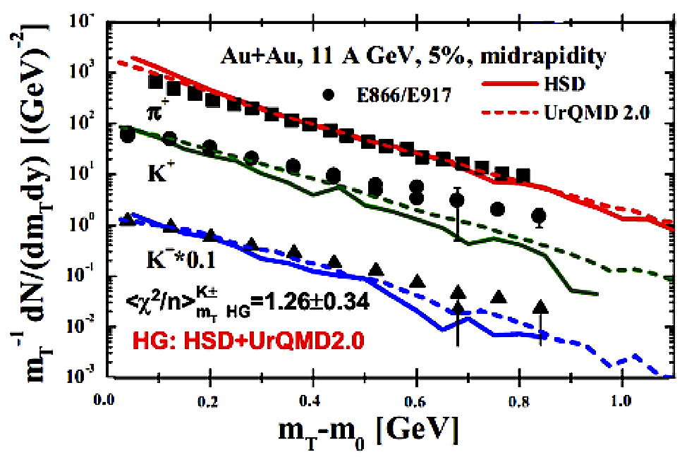
Figure 1: (Color online) Comparison of transverse mass spectra of $K^{+}$ and $K^{-}$ mesons at midrapidity from HSD (solid curves) and UrQMD 2.0 (dashed curves) for $\sqrt{s_{NN}}\,=$ 4.87 GeV taken from Fig. 7 of S4.9KL . The result for $\langle\chi^{2}/n\rangle^{K^{\pm}}_{m_{T}}\biggl{|}_{aa\overline{HG}}$ shown in this figure is described in the text.

The scan of curves and experimental data points allowed us to get the following results for the arithmetic averaging

$$\left.\begin{array}[]{l}\langle\chi^{2}/n\rangle^{K^{+}}_{m_{T}}\biggl{|}_{HSD}=1.9\pm 0.83\\ \langle\chi^{2}/n\rangle^{K^{+}}_{m_{T}}\biggl{|}_{UrQMD2.0}=1.05\pm 0.62\\ \end{array}\right\}~{}\Rightarrow~{}\langle\chi^{2}/n\rangle^{K^{+}}_{m_{T}}\biggl{|}_{aa\overline{HG}}=1.47\pm 0.52\,,$$ (13)

$$\left.\begin{array}[]{l}\langle\chi^{2}/n\rangle^{K^{-}}_{m_{T}}\biggl{|}_{HSD}=1.35\pm 0.7\\ \langle\chi^{2}/n\rangle^{K^{-}}_{m_{T}}\biggl{|}_{UrQMD2.0}=0.75\pm 0.52\\ \end{array}\right\}~{}\Rightarrow~{}\langle\chi^{2}/n\rangle^{K^{-}}_{m_{T}}\biggl{|}_{aa\overline{HG}}=1.05\pm 0.44\,.$$ (16)

Averaging the above results over types of hadrons one finds that $\langle\chi^{2}/n\rangle^{K^{\pm}}_{m_{T}}\biggl{|}_{aa\overline{HG}}=1.26\pm 0.34$. At the same time the weighted averaging gives us practically the same result $\langle\chi^{2}/n\rangle^{K^{\pm}}_{m_{T}}\biggl{|}_{wa\overline{HG}}=1.125\pm 0.32$.

In the same way we determined the QDD of the longitudinal rapidity distributions of kaons $\langle\chi^{2}/n\rangle^{K^{\pm}}_{y_{L}}\biggl{|}_{aa\overline{QGP}}$ for $\sqrt{s_{NN}}\,=$ 4.87 GeV using the results of QuarkComb. model QComb (see Fig. 2 and $K^{\pm}$ set 1 in Table I for details)

$$\left.\begin{array}[]{l}\langle\chi^{2}/n\rangle^{K^{+}}_{y_{L}}\biggl{|}_{QuarkComb}=4.47\pm 1.22\\ \langle\chi^{2}/n\rangle^{K^{-}}_{y_{L}}\biggl{|}_{QuarkComb}=0.236\pm 0.28\\ \end{array}\right\}~{}\Rightarrow~{}\langle\chi^{2}/n\rangle^{K^{\pm}}_{y_{L}}\biggl{|}_{{QuarkComb}}=2.353\pm 0.63\,.$$ (19)

The weighted averaging gives us a different result $\langle\chi^{2}/n\rangle^{K^{\pm}}_{y_{L}}\biggl{|}_{{QuarkComb}}=0.448\pm 0.273$, which within error bars is more close to the value of negative kaons in (19).

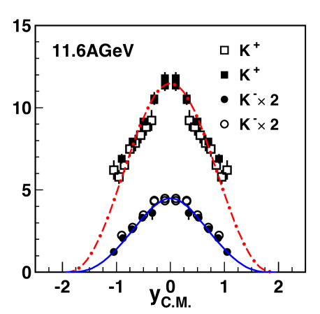
Figure 2: (Color online) The longitudinal rapidity spectra of $K^{+}$ and $K^{-}$ mesons (symbols) reproduced by the QuarkComb. model QComb . This is part of Fig. 5 of QComb which was used to determine $\langle\chi^{2}/n\rangle^{K^{\pm}}_{y_{L}}\biggl{|}_{aa\overline{QGP}}$.

Similarly, from Fig. 2 of S4.9KL we found the QDD of the midrapidity multiplicity of kaons for $\sqrt{s_{NN}}\,=$ 4.87 GeV, i.e. $\langle\chi^{2}/n\rangle^{K^{\pm}}_{\frac{dN}{dy}}\biggl{|}_{aa\overline{HG}}$. In particular, from Fig. 3 we determined the desired quantities for all values of collision energy given in this figure

$$\left.\begin{array}[]{l}\langle\chi^{2}/n\rangle^{K^{+}}_{\frac{dN}{dy}}\biggl{|}_{HSD}=12.44\pm 7.05\\ \langle\chi^{2}/n\rangle^{K^{+}}_{\frac{dN}{dy}}\biggl{|}_{UrQMD1.3}=0.32\pm 1.14\\ \langle\chi^{2}/n\rangle^{K^{+}}_{\frac{dN}{dy}}\biggl{|}_{UrQMD2.0}=14.62\pm 7.64\\ \end{array}\right\}~{}\Rightarrow~{}\langle\chi^{2}/n\rangle^{K^{+}}_{\frac{dN}{dy}}\biggl{|}_{aa\overline{HG}}=9.126\pm 3.5\,,$$ (23)

$$\left.\begin{array}[]{l}\langle\chi^{2}/n\rangle^{K^{-}}_{\frac{dN}{dy}}\biggl{|}_{HSD}=2.4\pm 3.1\\ \langle\chi^{2}/n\rangle^{K^{-}}_{\frac{dN}{dy}}\biggl{|}_{UrQMD1.3}=0.4\pm 1.27\\ \langle\chi^{2}/n\rangle^{K^{-}}_{\frac{dN}{dy}}\biggl{|}_{UrQMD2.0}=4.76\pm 4.36\\ \end{array}\right\}~{}\Rightarrow~{}\langle\chi^{2}/n\rangle^{K^{+}}_{\frac{dN}{dy}}\biggl{|}_{aa\overline{HG}}=2.52\pm 1.83\,.$$ (27)

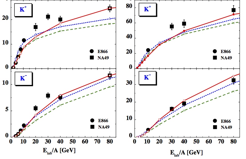
Figure 3: (Color online) The yields of $K^{+}$ and $K^{-}$ mesons (symbols) reproduced by the following HG models: HSD (solid curves), UrQMD1.3 (short dashed curve) and UrQMD2.1 (long dashed curve). The left column corresponds to the particle yields measured at midrapidity, while the right column gives the total yields in $4\pi$ solid angle. This is part of Fig. 2 of S4.9KL which was used to determine $\langle\chi^{2}/n\rangle^{K^{\pm}}_{\frac{dN}{dy}}\biggl{|}_{aa\overline{HG}}$ and $\langle\chi^{2}/n\rangle^{K^{\pm}}_{4\pi}\biggl{|}_{aa\overline{HG}}$ for all energies given in the plots.

In the same way we determined the arithmetic average of the QDD of the total $K^{\pm}$ multiplicities $\langle\chi^{2}/n\rangle^{K^{\pm}}_{4\pi}\biggl{|}_{aa\overline{HG}}$

$$\left.\begin{array}[]{l}\langle\chi^{2}/n\rangle^{K^{+}}_{4\pi}\biggl{|}_{HSD}=9.55\pm 6.2\\ \langle\chi^{2}/n\rangle^{K^{+}}_{4\pi}\biggl{|}_{UrQMD1.3}=1.\pm 2.\\ \langle\chi^{2}/n\rangle^{K^{+}}_{4\pi}\biggl{|}_{UrQMD2.0}=4.\pm 4.\\ \end{array}\right\}~{}\Rightarrow~{}\langle\chi^{2}/n\rangle^{K^{+}}_{4\pi}\biggl{|}_{aa\overline{HG}}=4.85\pm 2.55\,,$$ (31)

$$\left.\begin{array}[]{l}\langle\chi^{2}/n\rangle^{K^{-}}_{4\pi}\biggl{|}_{HSD}=0.67\pm 1.63\\ \langle\chi^{2}/n\rangle^{K^{-}}_{4\pi}\biggl{|}_{UrQMD1.3}=0.07\pm 0.54\\ \langle\chi^{2}/n\rangle^{K^{-}}_{4\pi}\biggl{|}_{UrQMD2.0}=1.2\pm 2.2\\ \end{array}\right\}~{}\Rightarrow~{}\langle\chi^{2}/n\rangle^{K^{-}}_{4\pi}\biggl{|}_{aa\overline{HG}}=0.646\pm 0.93\,.$$ (35)

From Eqs. (23) and (31) we found the corresponding average over two multiplicity sets for positive kaons, while Eqs. (27) and (35) allowed us to determine a similar average for negative kaons

$$\left.\begin{array}[]{l}\langle\chi^{2}/n\rangle^{K^{+}}_{aa\overline{\frac{dN}{dy}}}\biggl{|}_{aa\overline{HG}}=7.\pm 2.165\\ \langle\chi^{2}/n\rangle^{K^{-}}_{aa\overline{\frac{dN}{dy}}}\biggl{|}_{aa\overline{HG}}=1.6\pm 1.026\\ \end{array}\right\}~{}\Rightarrow~{}\langle\chi^{2}/n\rangle^{K^{\pm}}_{aa\overline{\frac{dN}{dy}}}\biggl{|}_{aa\overline{HG}}=4.3\pm 1.2\,,$$ (38)

where in the last step we averaged the results over two kinds of kaons. Repeating the same sequence of steps for the weighted averaging of Eqs. (6) and (7), we found $\langle\chi^{2}/n\rangle^{K^{\pm}}_{wa\overline{\frac{dN}{dy}}}\biggl{|}_{wa\overline{HG}}=0.5\pm 0.41$.

A few additional words should be said about various short hand notations used in Tables I and III-XI, which contain only the results of arithmetic averaging. Tables III-XI are given at the end of this work. To shorten our remarks inside these tables the sign $\&$ is used to demonstrate the fact that the corresponding value of $\langle\chi^{2}/n\rangle$ is averaged over two sets of data or over the results of models. For example, the notation $\frac{dN}{dy}\bigl{|}_{y=0}\&\quad 4\pi$ used in Table I shows that the value of $\langle\chi^{2}/n\rangle$ is averaged over the yields measured at midrapidity and in the full solid angle. Similarly, the notation ‘HSD & UrQMD2.0’ means that we give the value of $\langle\chi^{2}/n\rangle$ averaged over the results of models HSD and UrQMD2.0. In Table I, the notation ‘$m_{T}$+y’ made for $\Lambda$ hyperons (set 2) means that we give the value of $\langle\chi^{2}/n\rangle$ averaged over $m_{T}$- and y-distributions. More explaining remarks can be found in the captions of corresponding Tables.

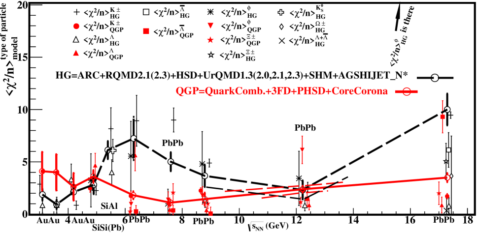
Figure 4: (Color online) KTBO plot 1: Comparison of $\langle\chi^{2}/n\rangle^{aa\overline{\{h\}}}_{aa\overline{\{A\}}}\biggl{|}_{aa\overline{HG}}$ (black symbols and dashed curve) and $\langle\chi^{2}/n\rangle^{aa\overline{\{h\}}}_{aa\overline{\{A\}}}\biggl{|}_{aa\overline{QGP}}$ (red symbols and solid curve) as functions of collision energy obtained for the arithmetic averaging. The symbols of different hadrons which correspond to the same collision energy are slightly spread around the energy value for better perception. The symbols are connected by the lines to guide the eye.

IV RESULTS

Our major results are shown in Figs. 4 and 6 and in Table II. The auxiliary results are given in the Tables I, III–XI. As one can see from the KTBO-plot 1, i.e. Fig. 4, there are several matches of the QDDs by HG and QGP models. At low collision energies the HG quantity $\langle\chi^{2}/n\rangle^{aa\overline{\{h\}}}_{aa\overline{\{A\}}}\biggl{|}_{aa\overline{HG}}$ is smaller than the one of QGP models, i.e. QDD is higher for HG generators. Although at energies below 4.87 GeV the QGP models are represented by the results of 3FD model, we stress that it would be extremely hard to reach a better description of the data by these models compared to the HG ones. It is so, since the latter provide almost an excellent description of the analyzed data for 3.1 GeV $\leq\sqrt{s_{NN}}\leq 4.2$ GeV, as one can see from Table II.

At the collision energies $\sqrt{s_{NN}}\,=$ 4.2 GeV ,$\sqrt{s_{NN}}\,=$ 4.87 GeV and $\sqrt{s_{NN}}\,=$ 12.3 GeV one finds

$$\langle\chi^{2}/n\rangle^{aa\overline{\{h\}}}_{aa\overline{\{A\}}}\biggl{|}_{aa\overline{HG}} = \langle\chi^{2}/n\rangle^{aa\overline{\{h\}}}_{aa\overline{\{A\}}}\biggl{|}_{aa\overline{QGP}}\,.$$ (39)

In the collision energy ranges 4.87 GeV $<\sqrt{s_{NN}}<$ 12.3 GeV and 12.3 GeV $<\sqrt{s_{NN}}<$ 17.3 GeV the QGP models describe the data essentially better. Therefore, the arithmetic averaging meta-analysis suggests that at energies below 4.2 GeV there is hadron phase, while in the region 4.2 GeV $\leq\sqrt{s_{NN}}\leq$ 4.87 GeV there is hadron-QGP mixed phase, while at higher energies there exists QGP. Such a picture is well fit into the recent findings of the generalized shock adiabat model Bugaev:2014a ; Bugaev:2014b . However, the most interesting question is how should we interpret the coincidence of two sets of results at the collision energy $\sqrt{s_{NN}}=$ 12.3 GeV?

 

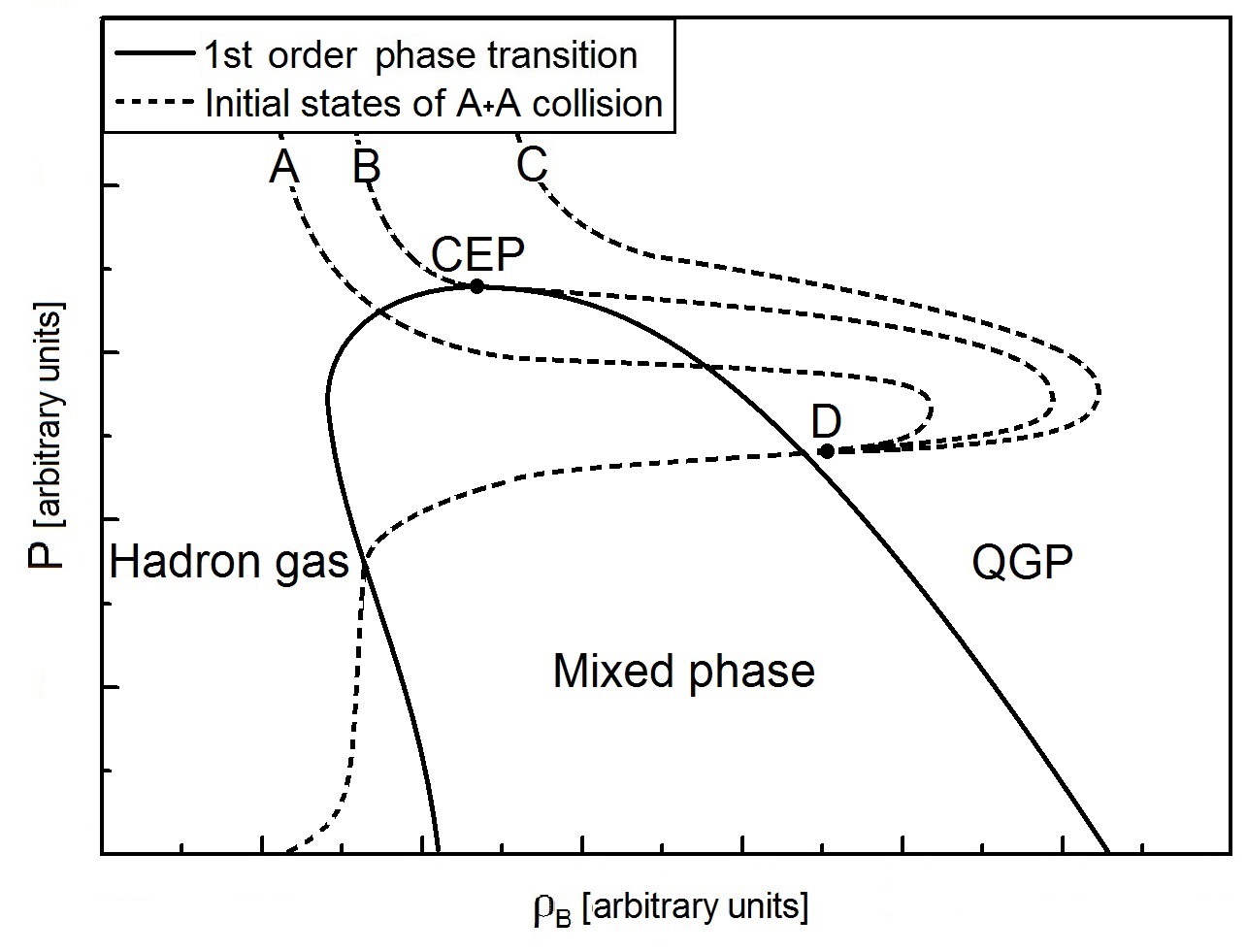
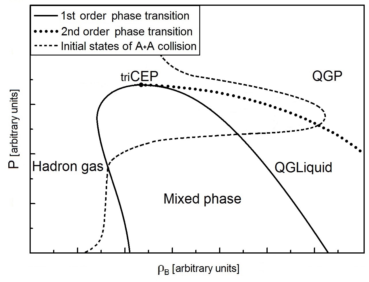
Figure 5: Schematic pictures of possible locations of the initial states of matter formed in A+A collisions are shown on the plane of baryonic density and pressure. Each point on these trajectories (dashed curves) corresponds to a single collision energy value. Left panel: As it is argued in the text the possible initial states correspond to the trajectories AD or BD as it follows from KTBO-plot 1 for the case of critical endpoint. The trajectory CD is located far from the mixed phase region and, hence, it cannot generate the second region in which the QDDs of HG and QGP models are equally good. Right panel: In case of the tricritical endpoint the second region in which the QDDs of HG and QGP models are equally good may, alternatively, appear due to the second phase transition.

At first glance it seems that at the collision energy $\sqrt{s_{NN}}=$ 12.3 GeV the QGP states created by the corresponding generators touch the phase boundary with hadron phase. However, one must remember that both curves depicted in Fig. 4 have, in fact, finite width defined by the error bars. Taking into account an overlap of the curves with finite error bars, one immediately concludes that the overlap region is rather wide on collision energy scale, namely it ranges from $\sqrt{s_{NN}}\simeq$ 10 GeV to $\sqrt{s_{NN}}\simeq$ 13.5 GeV. Recalling that the collision energy width of the mixed phase at low values of $\sqrt{s_{NN}}$ is below 1 GeV, one may guess that the most probable scenario is that the initial equilibrated states of the matter formed in A+A collisions at $\sqrt{s_{NN}}\simeq$ 10 GeV return into the hadron-QGP mixed phase, while at $\sqrt{s_{NN}}\simeq$ 13.5 GeV they return from the mixed phase into QGP.

From the present meta-analysis results it is hard to tell, whether the initial equilibrated states of the matter formed in A+A collisions at $\sqrt{s_{NN}}\in$ [10; 13.5] GeV reach the hadronic phase or they correspond to the mixed phase alone. However, such a wide range of collision energy of about 3.8 GeV should correspond to something entirely new, compared to the mixed phase located at the range $\sqrt{s_{NN}}\in$ [4.2; 4.87] GeV. We believe that the energy range $\sqrt{s_{NN}}\in$ [10; 13.5] GeV may correspond to the vicinity of the critical endpoint of the QCD phase diagram. The most probable locations on phase diagram of the initial states which formed in A+A collisions are schematically shown in the left panel of Fig. 5 in case of the critical endpoint. Our main reasons in favor of such a hypothesis are as follows. Recalling argumentation of Ref. Quarkyonic on the location of (tri)critical endpoint, we have to stress that the vicinity of collision energy 10 GeV was independently found in this work as the second entrance into the mixed phase from QGP. On the other hand, the lattice QCD results on the baryonic chemical potential $\mu_{B}$ dependence of pseudo-critical temperature $T_{ps}(\mu_{B})$ found from maximum of chiral susceptibility ChirSusc1 ; ChirSusc2 or from chiral limit ChirLim1 ; ChirLim2 show that the chemical freeze-out states at $\sqrt{s_{NN}}=$ 17.3 GeV Bugaev13:Horn ; Bugaev13:SFO correspond to the cross-over, but to the critical endpoint (see Karsch13 for an extended discussion). Therefore, we conclude that such a point should exist at collision energies below 17.3 GeV, i.e. close to the discussed region of collision energies.

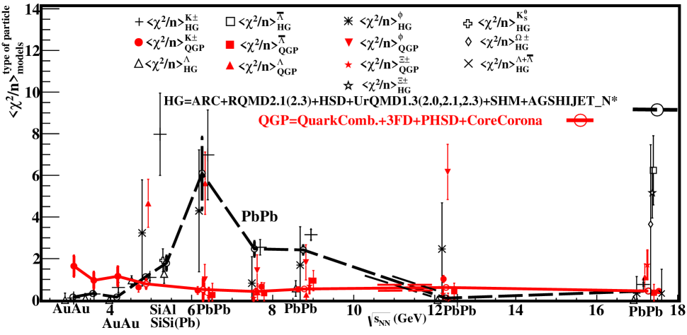
Figure 6: (Color online) KTBO plot 2: Comparison of $\langle\chi^{2}/n\rangle^{wa\overline{\{h\}}}_{wa\overline{\{A\}}}\biggl{|}_{wa\overline{HG}}$ (black symbols and dashed curve) and $\langle\chi^{2}/n\rangle^{wa\overline{\{h\}}}_{wa\overline{\{A\}}}\biggl{|}_{wa\overline{QGP}}$ (red symbols and solid curve) as functions of collision energy obtained for the wighted averaging. The symbols of different hadrons which correspond to the same collision energy are slightly spread around the energy value for better perception. The symbols are connected by the lines to guide the eye. The thin straight lines below collision energy 12 GeV demonstrate the intersection region due to finite error bars.

Of course, alternatively, the second mixed phase region found here at $\sqrt{s_{NN}}$= 10–13.5 $=11.75\pm 1.75$ GeV may correspond to the second phase transition (chiral), but even in this case the (tri)critical endpoint of the QCD phase diagram should be located nearby. Such a situation is depicted in the right panel of Fig. 5.

In order to better determine the energy range of the second entrance inside the mixed phase, let us verify our conclusions on the meta-analysis results shown in the KTBO-plot 2 (see Fig. 6). This KTBO-plot contains the meta-analysis results for the weighted averaging. Comparing KTBO-plot 1 and KTBO-plot 2 one can see that in many cases the values of $\langle\chi^{2}/n\rangle^{wa\overline{\{h\}}}_{wa\overline{\{A\}}}\biggl{|}_{wa\overline{QGP}}$ and $\langle\chi^{2}/n\rangle^{wa\overline{\{h\}}}_{wa\overline{\{A\}}}\biggl{|}_{wa\overline{HG}}$ are essentially smaller than the corresponding values obtained by the arithmetic averaging. This is a clear demonstration of the fact that the weighted averaging (6) and (7) ‘prefers’ the results with minimal error bars, which in our case means the smaller value of $\langle\chi^{2}/n\rangle^{h}_{A}\biggl{|}_{M}$ due to Eq. (2). Therefore, one has to be careful with this kind of averaging because at each energy there are only a few hadronic characteristics which have low value of $\langle\chi^{2}/n\rangle^{h}_{A}\biggl{|}_{M}$. Nevertheless, our main conclusions from this plot are qualitatively similar to the case of the KTBO-plot 1, although there are some quantitative difference. Thus, the equality

$$\langle\chi^{2}/n\rangle^{wa\overline{\{h\}}}_{wa\overline{\{A\}}}\biggl{|}_{wa\overline{HG}} = \langle\chi^{2}/n\rangle^{wa\overline{\{h\}}}_{wa\overline{\{A\}}}\biggl{|}_{wa\overline{QGP}}\,,$$ (40)

holds for the collisions energies $\sqrt{s_{NN}}\,=$ 4.87 GeV, $\sqrt{s_{NN}}\,=$10.8–12 GeV and $\sqrt{s_{NN}}\,=$ 17.3 GeV. Accounting for the finite error bars, we found that within the error bars the HG and QGP models describe the data equally well in the following region of collision energy: 4.4–5 GeV, 10.8–12 GeV and 14.3–17.3 GeV. In other words, within the present meta-analysis the region of energy $\sqrt{s_{NN}}=$ 4.2–4.87 GeV which we associated above with the hadron-QGP mixed phase remains almost the same, giving us the overlapping region of energies $\langle\sqrt{s_{NN}}\rangle_{overlap}=$ 4.4–4.87 GeV. However, instead of a single region of reentering the mixed phase now we found two ones. The most peculiar thing is that at the collision energies $\sqrt{s_{NN}}\,=$ 11.3–17.3 GeV the weighted averaging of HG models demonstrates somewhat better description of the data than the one of QGP models (see Fig. 6).

How can one understand these results? Our interpretation is as follows. We used two entirely different ways of averaging in order to study the stability of the results, and hence the most probable results of KTBO-plots 1and 2 are the ones which coincide. Therefore, the most probable energy range for the second mixed phase region is $\langle\sqrt{s_{NN}}\rangle_{overlap}=$ 10.8–12 = $11.4\pm 0.6$ GeV.

	Arithmetic averaging		Weighted averaging
$\sqrt{s_{NN}}$ (GeV)	HG models	QGP models	HG models	QGP models
3.1	$1.85\pm 0.575$	$4.1\pm 1.84$	$0.104\pm 0.077$	$1.62\pm 0.49$
3.6	$0.913\pm 0.442$	$3.976\pm 1.725$	$0.272\pm 0.1$	$0.94\pm 0.395$
4.2	$2.086\pm 0.762$	$2.616\pm 1.306$	$0.1042\pm 0.08$	$1.14\pm 0.46$
4.9	$2.813\pm 0.9$	$3.57\pm 0.608$	$1.086\pm 0.13$	$0.772\pm 0.22$
5.4	$6.1\pm 0.854$	N/A	$1.733\pm 0.346$	N/A
6.3	$7.24\pm 2.06$	$1.78\pm 0.37$	$6.044\pm 1.737$	$0.493\pm 0.54$
7.6	$5\pm 0.9$	$1.08\pm 0.27$	$2.4\pm 0.358$	$0.405\pm 0.126$
8.8	$3.66\pm 1.06$	$1.41\pm 0.613$	$2.355\pm 0.208$	$0.53\pm 0.1$
12.3	$2.29\pm 0.9$	$2.38\pm 0.33$	$0.0564\pm 0.027$	$0.6\pm 0.11$
17.3	$10\pm 1.51$	$3.475\pm 0.427$	$0.38\pm 0.0531$	$0.434\pm 0.12$

Table 2: The resulting QDD values provided by two ways of averaging. These results of HG and QGP models are shown in KTBO-plots 1 and 2.

As an independent check up, let us consider the energy ranges $\sqrt{s_{NN}}=\{11.75\pm 1.75;11.4\pm 0.6;15.5\pm 1.5\}$ GeV of the second mixed phase region which we found from the KTBO-plots 1 and 2 as the results of independent meta-measurements. Then applying to them the both ways of averaging, i.e. using Eqs. (4) and (6), we obtain

$$\langle\sqrt{s_{NN}}\rangle_{aa}=12.9\pm 0.8~{}{\rm GeV}\,,\quad\langle\sqrt{s_{NN}}\rangle_{wa}=11.95\pm 0.53~{}{\rm GeV}\,.$$ (41)

The weighted averaging in (41) gives us nearly the same estimate which we found from the overlapping regions in the KTBO-plots 1 and 2, while the arithmetic averaging provides us with a more conservative estimate. We suggest to use this value $\langle\sqrt{s_{NN}}\rangle_{aa}=12.9\pm 0.8$ GeV as the most probable estimate for the (tri)critical endpoint collision energy. The main reason is that the two other estimates, i.e. $\langle\sqrt{s_{NN}}\rangle_{overlap}=11.4\pm 0.6$ GeV and $\langle\sqrt{s_{NN}}\rangle_{wa}=11.95\pm 0.53$ GeV, correspond to the second mixed phase region and, hence, it is logical to assume that the (tri)critical endpoint energy is located more close to the upper boundary of these estimates or even at a slightly higher energy. This is exactly the region provided by the arithmetic averaging of the collision energy values. Also such a conclusion is supported by the fact that the endpoint was, so far, not found at $\sqrt{s_{NN}}=$ 11.5 GeV and $\sqrt{s_{NN}}=$ 12.3 GeV. Recall also the main conclusion of RHIC Beam Energy Scan Mohanty13 that the properties of strongly interacting matter created in A+A collisions at energies below and above $\sqrt{s_{NN}}\,=\,11.5$ GeV are different. Hence, the value $\langle\sqrt{s_{NN}}\rangle_{aa}=12.9\pm 0.8$ GeV is the present days best estimate which is provided by the suggested meta-analysis. Hopefully, it can be improved further, if one accounts for the RHIC Beam Energy Scan results measured at the collision energies $\sqrt{s_{NN}}=11.5$ GeV and $\sqrt{s_{NN}}=19.6$ GeV.

V Conclusions and Perspectives

Here we performed the meta-analysis of the QDD of the existing A+A event generators without and with QGP existence which allow one to extract physical information of principal importance. These kinds of generators are, respectively, called the HG and QGP model. A priori we assumed that, despite their imperfectness, these models contain the grain of truth on the QGP formation in central nuclear collisions which we would like to distillate using the suggested meta-analysis. For each collision energy we consider the set of QDD $\langle\chi^{2}/n\rangle^{h}_{A}\biggl{|}_{M}$ of the experimental quantity $A$ of hadron $h$ described by the model $M\in\{HG;QGP\}$ as the results of independent meta-measurements. The studied experimental quantities include the transverse mass spectra, the longitudinal rapidity distributions and yields measured at midrapidity and/or in the full solid angle. In this work we analyzed the strange hadrons only, since they provide us with one of the most popular probes both of experimental measurements and of theoretical investigations. Using two ways of averaging for the QDD $\langle\chi^{2}/n\rangle^{h}_{A}\biggl{|}_{M}$ and its error, we were able to extract the QDD by two kinds of models at each collision energy.

Comparing the results found by these two kinds of models we were able to locate the regions of their equal QDD at the collision energies $\langle\sqrt{s_{NN}}\rangle_{overlap}=$ 4.4–4.87 GeV and $\langle\sqrt{s_{NN}}\rangle_{overlap}=$ 10.8–12 GeV, which we identified with the mixed phase regions. As expected, at center of mass energies below 4.2 GeV the HG models ‘work’ better than the QGP ones. As it is seen from the KTBO-plots 1 and 2, in the collision energy range $\sqrt{s_{NN}}\,=$ 5–10.8 GeV the HG models fail to reproduce the vast majority of data, while the QGP models reproduce data rather well. Therefore, this region we associated with QGP. Unfortunately, results of the A+A event generators used here did not allow us yet to uniquely interpret our findings at the collision energies above 12 GeV. Our educated guess is that the energy range $\langle\sqrt{s_{NN}}\rangle_{aa}=12.9\pm 0.8$ GeV corresponds to the vicinity of the (tri)critical endpoint. Such a guess is, on the one hand, supported by the phenomenological arguments of Ref. Quarkyonic on the location of (tri)critical endpoint. On the other hand, our hypothesis is also confirmed by the results of lattice QCD ChirSusc1 ; ChirSusc2 ; ChirLim1 ; ChirLim2 that the chemical freeze-out states at $\sqrt{s_{NN}}=$ 17.3 GeV belong to the cross-over region and, hence, the (tri)critical endpoint should be located at lower energies of collision.

Of course, the energies $\langle\sqrt{s_{NN}}\rangle_{aa}=12.97\pm 0.92$ GeV may correspond to the second phase transition of QCD, but even in this case the (tri)critical endpoint of the QCD phase diagram should be located nearby. Perhaps, our findings may help to interpret the conclusions of the RHIC Beam Energy Scan Program Mohanty13 that below and above $\sqrt{s_{NN}}\,=\,11.5$ GeV one, respectively, probes the different phases of QGP which have different properties. We hope that this question could be answered, if the RHIC Beam Energy Scan data measured at center of mass energies 11.5 GeV and 19.7 GeV were analyzed by the event generators and then reanalyzed using the present approach. We would like to stress that the present work strongly supports conclusions of the generalized shock adiabat model Bugaev:2014a ; Bugaev:2014b that the hadron-QGP mixed phase is located between the center of mass energies 4.2 GeV and 4.87 GeV. On the other hand, there is absolutely no evidence for the onset of deconfinement at the center of mass collision energy 7.6 GeV, as it is claimed in Horn ; Step ; Gazd_rev:10 . Therefore, we believe that without establishing a much more convincing relation between the irregularities discussed in Gazd_rev:10 and the deconfinement phase transition one simply cannot consider them to be signals of deconfining transition.

The current set of analyzed models does not cover the full spectrum of existing ones, but already this sample was sufficient to obtain interesting results and show the power of the suggested meta-analysis. Also it is worth to note that to essentially change the results of present meta-analysis it would be necessary to greatly improve the description of existing data either by HG models in the center of mass collision energy range 5.4–12.3 GeV or by QGP models at energies below 4.2 GeV. Otherwise, it would be hard to change the obtained results, since they are based on the analysis of more than 100 different experimental data sets.

Due to absence of necessary information on the QDD of A+A collisions, we were forced to make the tantalizing efforts in order to scan both the experimental data and their description by the event generators of such collisions from the published figures. Such efforts could be avoided, if all existing experimental data on A+A collisions were collected together like it is done in the Particle Data Group for collisions of elementary particles. Also the success of present meta-analysis suggests that the results of theoretical works which describe data should be presented not only in figures, but also they should be available as the numbers in the form of QDD $\langle\chi^{2}/n\rangle^{h}_{A}\biggl{|}_{M}$ and as the total mean deviation squared per degree of freedom (if such a number can be found). Then the first of them can be used for the meta-analysis we performed here, while the second ones will help us to determine the most successful A+A event generators of available data. Such an information can be used for planning the collision energy of ongoing experiments and for further improvement of the existing A+A event generators. We believe that only along this way the heavy ion collisions community will be able to solve its ultimate tasks, i.e. to locate the hadron-QGP mixed phase and to discover the QCD phase diagram endpoint. Therefore, as the first step in this direction in Tables I and III-XI we present the values of QDD used in our meta-analysis for the arithmetic averaging along with the final values for the both ways of averaging used in the KTBO-plots 1 and 2 (see Table II). The values of QDD obtained for the weighted averaging will be published elsewhere.

As the first practical steps we suggest to the RHIC Beam Energy Scan Program to make a few measurements in the center of mass collision energy ranges from 3.9 GeV to 5.15 GeV and from 10.8 GeV to 15.5 GeV. The first of them may lead to a discovery of the hadron-QGP mixed phase, while the second one may lead to a location of the QCD phase diagram endpoint.

Acknowledgements. The authors would like to thank M. Bleicher, A.I. Ivanytskyi, L.M. Satarov and A. Taranenko for fruitful discussions. Special thanks go to D. H. Rischke for his valuable comments. This work was supported in part by the Program of Fundamental Research of the Department of Physics and Astronomy of NAS of Ukraine. K.A.B. acknowledges a partial support provided by the Helmholtz International Center for FAIR within the framework of the LOEWE program launched by the State of Hesse.

VI Appendix: Description of the models compared

Here we briefly discuss characteristics of the models used in the present meta-analysis. We have to apologize for giving a few basic references only. The main criterion for choosing these models was the wide acceptance of their results by heavy ion community and a requirement that their results are well documented. In our analysis we on purpose included not only cascades, hadronic or partonic, but also statistical (SHM) and hydrodynamical (3FD) models, since we believe that the meta-analysis works better, if the models of different kinds are included. We consider a model to be of a QGP type, if in it, explicitly or implicitly, there appears a dense medium of quarks and gluons (partons), whose properties are entirely different from the ones of hadronic medium employed in this model.

ARC (A Relativistic Cascade) Arc ; Schlagel:1992fh is a purely hadronic cascade, developed in the Brookhaven National Laboratory in the early 90s. ARC is designed for and limited to AGS energies. It does not include any potentials, mean field effects, off-shellness, strings or in-medium effects. Hadrons participate in $2\to 2$ elastic and inelastic collisions, resonance formations and decays. Cross-sections and their parameterizations are taken from CERN-HERA and LBL compilations as well as from papers ARC_cross_sections . Collisions are triggered using a geometrical criterion: if distance between particles $r_{ij}\leq(\sigma_{ij}/\pi)^{1/2}$, where $\sigma_{ij}$ is corresponding total cross-section, then collision happens. Formation time of 1 fm/c is introduced. Apparently, this is a HG model.

RQMD (Relativistic Quantum Molecular Dynamics) Sorge:1989vt ; Sorge:1995dp is a hadron cascade, developed since 1989 in the Institute of Theoretical Physics of the University of Frankfurt upon Main. It employs nuclear potentials, implemented in a Lorentz-covariant manner, at low energies and fills cross-section with interacting strings at higher energies. Interactions of energy up to 2-3 GeV mainly proceed through hadronic resonances, such as $\rho$, $\eta$, $K^{*}$, $\phi$, $\Delta$, $N^{\prime}$, parametrized by many-channels Breit-Wigner formula. Unknown cross-sections are calculated using additive quark model, namely, $\sigma_{tot}\sim(1-0.4x_{1})(1-0.4x_{2})$, where $x_{1,2}=\frac{N_{s}}{N_{u}+N_{d}}$ - strange to non-strange quarks ratio in the corresponding hadron. Like in ARC, there is a formation time of 1 fm/c and geometrical collision criterion. Hadronic cross-sections are taken from different sources, compared to ARC RQMD_cross_sections . At higher energies interactions go via strings using phenomenological Lund model, extended by possibility for strings to interact, forming so-called ropes (see Bierlich:2014xba for review). RQMD is often believed to be valid at a broad collision energies range from $\sim$50 MeV to hundreds GeV per nucleon.

UrQMD (Ultra-relativistic Quantum Molecular Dynamics) is a successor of RQMD, developed in Frankfurt ITP in the late 90s Bass98 . Most recent version can be run as a hybrid model, but we consider only earlier pure hadronic cascade versions. Unlike RQMD, UrQMD employs non-relativistic nuclear potentials, that are switched off at relative momentum of colliding hadrons above 2 GeV. Resonance table is significantly improved compared to RQMD. Cross-sections are mainly taken from Particle Data Group (PDG) and CERN-HERA compilations and are parametrized using multi-channel Breit-Wigner ansatz. Experimentally unknown channels, such as resonance-resonance or hyperon-resonance scattering, are parametrized using phenomenological additive quark model. As RQMD and HSD, UrQMD employs Lund string model at center of mass collision energies $\sqrt{s_{NN}}>3$ GeV. Unlike RQMD, UrQMD strings do not interact.

HSD (Hadron String Dynamics) is a hadron cascade developed at Giessen in the mid-90s HSDgen ; S5.4a . It employs potentials, implemented as a relativistic mean-field. HSD particles propagate off-shell and their self-energies are modified in the medium. In the hadronic scattering part HSD is the successor of BUU code, developed by the Giessen group Wolf:1993pja . Collisions happen according to the geometrical criterion, as in ARC and RQMD. Cross-sections are taken from similar sources to ARC plus CERN ISR compilation. In some cases strange particle cross-sections are re-parametrized to change cross-section behavior in the energy regions, where data are not available Cassing:1996xx . At the center of mass collision energies of nucleons higher than 2.6 GeV interaction proceeds via strings HSDgen , operating according to Lund string model. Strings cannot interact: ropes and string fusion like in RQMD are not implemented. Parameters of Lund model are changed from energy to energy to match experimental data S5.4a .

AGSHIJET HIJETa is a hadron cascade inheriting from HIJET Shor:1988vk , which, in turn, comes from a ISAJET generator for $p+p$ collisions Paige:1986kt . All these models were developed at Brookhaven National Laboratory in late 80s - early 90s. AGSHIJET operates with strings and uses not the Lund model, but a Field-Feynmann model, which has a different parametrization for fragmentation functions. HIJET simulates A+A collision as a sequence of independent $NN$ collisions, where individual $NN$ collisions are treated using ISAJET. Further HIJET applies a hadron cascade, similar to ARC, to the obtained products. In the AGSHIJET resonance treatment was improved, $N^{*}$ added and Field-Feynmann model parameters were adjusted to reproduce $p+p$ reaction cross-section at laboratory frame momentum below 50 GeV.

SHM (Statistical Hadronization Model) is not a microscopic, but a pure statistical model of hadron gas Becattini:2003wp ; SHMgen , which allows one to obtain hadron yields (but not spectra) under the assumption of a sharp chemical freeze-out. In this model it is assumed that before chemical freeze-out matter is in thermal and chemical equilibrium and after it inelastic reactions are frozen and only resonance decays and elastic reactions occur. Thermal yields of hadrons are calculated from the equilibrium ideal gas partition function and read as $N=\frac{gV|\gamma_{s}|^{n_{s}}}{2\pi^{2}}\int\frac{k^{2}dk}{e^{(E-\mu)/T}\pm 1}$. Temperature $T$, volume $V$, baryon chemical potential $\mu$ and strangeness suppression factor $\gamma_{s}$ are free parameters, adjusted at each collision energy to provide the best fit of experimental hadronic yields. Interaction between hadrons is taken into account via adding resonances as independent components of ideal gas.

QuarkComb (Quark Combination model) QComb is a phenomenological gluonless model, which generates effective quarks with rapidity distribution of $\frac{dN_{q}}{N_{q}\,dy}=B\left(e^{-|y|^{a}/2\sigma^{2}}-e^{-|y_{beam}|^{a}/2\sigma^{2}}\right)$, where $B$ is normalization constant, while $a$ and $\sigma$ are adjustable parameters. Number and flavour of quarks are generated according to a phenomenological model of hadronization introduced by Xie and Liu in 1988 Xie:1988wi and tuned to describe hadron production in $e^{+}+e^{-}$ collisions. Effective (anti)quarks are sorted in rapidity and neighbors in the array are combined into mesons or baryons: $qq\bar{q}$ and its permutations give a meson and one quark remains in the array, while $qqq$ gives a baryon. To obtain final spectra hadron resonances are decayed. According to our criterion this is QGP model.

3FD (3-fluid dynamics) is a hydrodynamical model of heavy ion collision, developed by Ivanov and Russkikh 3FDgen . It considers ion collision as three fluids: two baryon-rich fluids corresponding to projectile and target and the third one, corresponding to produced particles. A following system of coupled equations of perfect fluid dynamics

$$\partial_{\mu}T^{\mu\nu}_{p} = -F_{p}^{\nu}+F_{fp}^{\nu}\,,$$ (42)

$$\partial_{\mu}T^{\mu\nu}_{t} = -F_{t}^{\nu}+F_{ft}^{\nu}\,,$$ (43)

$$\partial_{\mu}T^{\mu\nu}_{f} = F_{p}^{\nu}-F_{fp}^{\nu}+F_{t}^{\nu}-F_{ft}^{\nu}\,,$$ (44)

is solved for the equation of state with the first order phase transition between hadronic matter and QGP 3FDII ; 3FDIII . The left hand side of system (42) is standard for relativistic hydrodynamics, while its right hand side represents interaction between fluids. Since $\partial_{\mu}(T^{\mu\nu}_{p}+T^{\mu\nu}_{t}+T^{\mu\nu}_{f})=0$, total energy and momentum are conserved. Freeze-out is performed using a modified Cooper-Frye procedure and, hence, it experiences the typical problems of other hydrodynamic models discussed in Freeze:96 . After freeze-out the obtained resonances are decayed. For considered two phase equation of state we assign 3FD approach to QGP models.

PHSD (Parton-Hadron-String Dynamics) PHSDgen is the most advanced cascade model based on HSD. It combines the HSD hadronic sector with a new model for partonic transport and hadronization, so-called DQPM (Dynamical Quasi-Particle Model). DQPM describes QCD properties in terms of single-particle Green’ s functions (in the sense of a two-particle irreducible approximation). Elastic and inelastic $q+q\leftrightarrow q+q$, $g+g\leftrightarrow g+g$, $g+g\leftrightarrow g$, $q+\bar{q}\leftrightarrow g$ reaction are included, fulfilling the detailed balance condition. Hadronization is occurring continuously based on Lorentz-invariant transition rates. Obtained hadron is embedded to the HSD cascade. If the hadron mass is too large, then it is considered as a HSD string. Apparently, this is QGP model.

Core-Corona Model CoreCorMa is a phenomenological approach suggested in 2005 to parameterize and to represent experimental data in a simple, but effective way. It was further developed in CoreCorMb . This model is based on the assumption that the fireball created in nuclear collisions is composed of a core, which has the same properties as a very central collision system, and a corona, which has different properties and is considered as a superposition of independent nucleon-nucleon interactions. The sizes of core and corona are defined by the condition that the corona is formed by those nucleon-nucleon collisions in which both participants interact only once during the entire process of A+A collision. The fraction of single scatterings is calculated using straight line geometry as described in the Glauber model Glauber . Since nowadays there are no doubts that at sufficiently high energies in central A+A collisions the QGP is formed, therefore at such energies we regard a core state of this model as an implicit parameterization of QGP state.

	$\sqrt{s_{NN}}\,=$ 3.1 GeV
	$m_{T}$-distribution	rapidity distribution	Yields
$\langle\chi^{2}/n\rangle=$			$0.856\pm 0.755$ $\left(\frac{dN}{dy}\bigl{|}_{y=0}\&\quad 4\pi\right)$
$\Lambda(\Sigma^{0})$	N/A	N/A	HSD & UrQMD1.3(2.1)
			Figs. 1, Ref. S4.9KL
$\langle\chi^{2}/n\rangle=$	$1.575\pm 0.724$		$5.9\pm 4.85$
$K^{+}$ set1	3FD	N/A	3FD
	Fig. 1, Ref. 3FDIII		Fig. 9, Ref. 3FDII
$\langle\chi^{2}/n\rangle=$	$1.49\pm 0.676$		$7.43\pm 5.45$
$K^{-}$ set1	3FD	N/A	3FD
	Fig. 1, Ref. 3FDIII		Fig. 9, Ref. 3FDII
$\langle\chi^{2}/n\rangle=$	$1.35\pm 0.476$		$8.246\pm 3.316$ $\frac{dN}{dy}\bigl{|}_{y=0}$
$K^{+}$ set 2	HSD & UrQMD2.0	N/A	HSD & UrQMD1.3(2.1)
			Fig. 1 or 2, Ref. S4.9KL
$\langle\chi^{2}/n\rangle=$	$1.7\pm 0.51$		$0.0714\pm 0.31$ $\frac{dN}{dy}\bigl{|}_{y=0}$
$K^{-}$ set 2	HSD & UrQMD2.0	N/A	HSD & UrQMD1.3(2.1)
			Figs.1 or 2, Ref. S4.9KL
$\langle\chi^{2}/n\rangle=$	$1.525\pm 0.35$
$K^{\pm}$	HSD & UrQMD2.0	N/A	N/A
	Fig. 7, Ref. S4.9KL

Table 3: Same as in Table 1, but for collision energy $\sqrt{s_{NN}}\,=$ 3.1 GeV.

	$\sqrt{s_{NN}}\,=$ 3.6 GeV
	$m_{T}$-distribution	rapidity distribution	Yields
$\langle\chi^{2}/n\rangle=$			$0.862\pm 0.76$ $\left(\frac{dN}{dy}\bigl{|}_{y=0}\&\quad 4\pi\right)$
$\Lambda(\Sigma^{0})$	N/A	N/A	HSD & UrQMD1.3(2.1)
			Figs. 1, Ref. S4.9KL
$\langle\chi^{2}/n\rangle=$	$5.53\pm 2.74$		$2.13\pm 1.7$ $\left(\frac{dN}{dy}\bigl{|}_{y=0}\right)$
$K^{+}$ set 1	$m_{T}$-distr.+Yield:3FD	N/A	HSD & UrQMD1.3(2.1)
	$m_{T}$:Fig.1,Ref.3FDIII ;Yield:Fig.9,Ref.3FDII		Fig. 1 or 2, Ref. S4.9KL
$\langle\chi^{2}/n\rangle=$	$1.17\pm 0.46$
$K^{+}$ set 2	HSD & UrQMD2.0	N/A	N/A
	Fig. 7, Ref. S4.9KL
$\langle\chi^{2}/n\rangle=$	$0.453\pm 0.286$		$0.0824\pm 0.332$ $\left(\frac{dN}{dy}\bigl{|}_{y=0}\right)$
$K^{-}$ set1	HSD & UrQMD2.0	N/A	HSD & UrQMD1.3(2.1)
	Fig. 7, Ref. S4.9KL		Fig. 1 or 2, Ref. S4.9KL
$\langle\chi^{2}/n\rangle=$	$0.494\pm 0.424$		$4.35\pm 4.17$
$K^{-}$ set2	3FD	N/A	3FD
	Fig. 1, Ref. 3FDIII		Fig. 9, Ref. 3FDII
	$\sqrt{s_{NN}}\,=$ 4.2 GeV
	$m_{T}$-distribution	rapidity distribution	Yields
$\langle\chi^{2}/n\rangle=$			$3.35\pm 1.47$ $\left(\frac{dN}{dy}\bigl{|}_{y=0}\&\quad 4\pi\right)$
$\Lambda(\Sigma^{0})$	N/A	N/A	HSD & UrQMD1.3(2.1)
			Fig. 1, Ref. S4.9KL
$\langle\chi^{2}/n\rangle=$	$0.81\pm 0.3$		$0.8343\pm 0.75$ $\left(\frac{dN}{dy}\bigl{|}_{y=0}\right)$
$K^{\pm}$	HSD & UrQMD2.0	N/A	HSD & UrQMD1.3(2.1)
	Fig. 7, Ref. S4.9KL		Fig. 1 or 2, Ref. S4.9KL
$\langle\chi^{2}/n\rangle=$	$3.367\pm 1.22$		$5.7\pm 4.78$
$K^{+}$	3FD	N/A	3FD
	Fig. 1, Ref. 3FDIII		Fig. 9, Ref. 3FDII
$\langle\chi^{2}/n\rangle=$	$0.73\pm 0.54$		$.665\pm 1.63$
$K^{-}$	3FD	N/A	3FD
	Fig. 1, Ref. 3FDIII		Fig. 9, Ref. 3FDII

Table 4: Same as in Table 1, but for collision energies $\sqrt{s_{NN}}\,=$ 3.6 and 4.2 GeV.

	$\sqrt{s_{NN}}\,=$ 5.4 GeV
	$m_{T}$-distribution	rapidity distribution	Yields
$\langle\chi^{2}/n\rangle=$		$8.17\pm 2$
$K^{\pm}$	N/A	HSD	N/A
		Fig. 14, Ref. S5.4a
$\langle\chi^{2}/n\rangle=$		$0.45\pm 0.6,$ $1.64\pm 1.14$	$1.1\pm 2.1,$ $1.35\pm 2.3$
$\Lambda$ set 1	N/A	ARC(SiSi(Pb))	ARC(SiSi(Pb))
		Figs. 4-5, Ref. S5.4b	Ref. S5.4b
$\langle\chi^{2}/n\rangle=$		$2.24\pm 1.3,$ $6.1\pm 2.2$	$8.9\pm 6,$ $10.2\pm 6.4$
$\Lambda$ set 2	N/A	AGSHIJET-N*(SiSi(Pb))	AGSHIJET-N*(SiSi(Pb))
		Figs. 4-5, Ref. S5.4b	Ref. S5.4b
$\langle\chi^{2}/n\rangle=$		$11.7\pm 3,$ $22\pm 4$	$1\pm 2,$ $0.3\pm 1$
$K_{S}^{0}$	N/A	ARC(SiSi(Pb))	ARC(SiSi(Pb))
		Figs. 2-3, Ref. S5.4b	Ref. S5.4b
$\langle\chi^{2}/n\rangle=$		$1.06\pm 0.9,$ $2.4\pm 1.4$	$3.5\pm 3.7,$ $7\pm 5$
$\Lambda$ set 3	N/A	AGSHIJET-N*(SiSi(Pb))	AGSHIJET-N*(SiSi(Pb))
		Figs. 2-3, Ref. S5.4b	Ref. S5.4b

Table 5: Same as in Table 1, but for the collision energy $\sqrt{s_{NN}}\,=$ 5.4 GeV. The notation ‘ARC(SiSi(Pb))’ used for $\Lambda$ hyperons (set 1) of $y$-distribution means that at preceding row of this column we give two values of $\langle\chi^{2}/n\rangle$ which correspond to Si+Si and Si+Pb collisions calculated for the event generator ARC.

	$\sqrt{s_{NN}}\,=$ 6.3 GeV
	$m_{T}$-distribution	rapidity distribution	Yields
$\langle\chi^{2}/n\rangle=$	$1.215\pm 0.73$	$2.28\pm 0.522$
$K^{\pm}$	$m_{T}$-distr.+Yield:3FD	QuarkComb. model	N/A
	$m_{T}$:Fig.1,Ref.3FDIII ;Yield:Fig.9,Ref.3FDII	Fig. 2 Ref. QComb
$\langle\chi^{2}/n\rangle=$		$1\pm 0.72$	$2.91\pm 3.41,$ $8.2\pm 5.73$
$\phi$	N/A	QuarkComb. model	SHM, UrQMD
		Fig. 2 Ref. QComb	Fig. 17 Ref. Blume
$\langle\chi^{2}/n\rangle=$		$5.645\pm 1.5$
$\Lambda$	N/A	QuarkComb. model	N/A
		Fig. 2, Ref. QComb
$\langle\chi^{2}/n\rangle=$		$0.266\pm 0.516$
$\bar{\Lambda}$	N/A	QuarkComb. model	N/A
		Fig. 2, Ref. QComb
$\langle\chi^{2}/n\rangle=$		$0.277\pm 0.39$
$\Xi^{-}$	N/A	QuarkComb. model	N/A
		Fig. 2, Ref. QComb

Table 6: Same as in Table 1, but for the collision energy $\sqrt{s_{NN}}\,=$ 6.3 GeV.

	$\sqrt{s_{NN}}\,=$ 7.6 GeV
	$m_{T}$-distribution	rapidity distribution	Yields
$\langle\chi^{2}/n\rangle=$	$1.51\pm 0.53$	$0.6\pm 0.265$
$K^{\pm}$	3FD	QuarkComb. model	N/A
	Fig. 1, Ref. 3FDIII	Fig. 2 Ref. QComb
$\langle\chi^{2}/n\rangle=$		$1.413\pm 0.752$	$0.567\pm 1.5,$ $1.44\pm 2.4$
$\phi$	N/A	QuarkComb. model	SHM,UrQMD
		Fig. 2, Ref. QComb	Fig. 17, Ref. Blume
$\langle\chi^{2}/n\rangle=$		$0.4\pm 0.4$
$\Lambda$	N/A	QuarkComb. model	N/A
		Fig. 2, Ref. QComb
$\langle\chi^{2}/n\rangle=$		$0.363\pm 0.5$
$\bar{\Lambda}$	N/A	QuarkComb. model	N/A
		Fig. 2, Ref. QComb
$\langle\chi^{2}/n\rangle=$		$2.16\pm 0.856$
$\Xi^{\pm}$	N/A	QuarkComb. model	N/A
		Fig. 2, Ref. QComb

Table 7: Same as in Table 1, but for the collision energy $\sqrt{s_{NN}}\,=$ 7.6 GeV.

	$\sqrt{s_{NN}}\,=$ 8.8 GeV
	$m_{T}$-distribution	rapidity distribution	Yields
$\langle\chi^{2}/n\rangle=$	$4.03\pm 0.9$	$2.76\pm 0.56,$ $3.826\pm 0.654$	$0.1\pm 0.3$
$K^{\pm}$ set 1	3FD	HSD, PHSD	Core Corona
	Fig.1,Ref. 3FDIII	Fig. 15 Ref. Phsd	Fig. 10 Ref. CoreCor
$\langle\chi^{2}/n\rangle=$	$2.33\pm 0.7$	$0.98\pm 0.333$	$10.7\pm 0.7$
$K^{\pm}$ set 2	PHSD	QuarkComb. model	y+Yield: HSD & UrQMD2.3
	Fig. 16 Ref. Phsd	Fig. 2 Ref. QComb	Figs. 6-7,10 Ref. CoreCor
$\langle\chi^{2}/n\rangle=$		$1.8\pm 0.846$	$0.94\pm 1.94,$ $8.614\pm 5.9$
$\phi$	N/A	QuarkComb. model	SHM,UrQMD
		Fig. 2, Ref. QComb	Fig. 17, Ref. Blume
$\langle\chi^{2}/n\rangle=$		$1.51\pm 0.78,$ $0.185\pm 0.27;$ $0.6\pm 0.5$
$\Lambda(\Sigma^{0})$	N/A	HSD, PHSD; QuarkComb. model	N/A
		Fig. 17 Ref. Phsd ; Fig. 2 Ref. QComb
$\langle\chi^{2}/n\rangle=$		$2.535\pm 1.126,$ $0.586\pm 0.54$
$\bar{\Lambda}$	N/A	PHSD, QuarkComb. model	N/A
		Fig. 18 Ref. Phsd , Fig. 2 Ref. QComb
$\langle\chi^{2}/n\rangle=$		$1.14\pm 0.7,$ $0.95\pm 0.667$
$\Xi^{\pm}$	N/A	PHSD, QuarkComb. model	N/A
		Figs. 19-20 Ref. Phsd , Fig. 2 Ref. QComb

Table 8: Same as in Table 1, but for the collision energy $\sqrt{s_{NN}}\,=$ 8.8 GeV. The notation ‘y+Yield’ used for $K^{\pm}$ mesons (set 2) means that we show the value of $\langle\chi^{2}/n\rangle$ averaged over the y-distribution and the particles yield, first, and then the results obtained for positive and negative kaons are arithmetically averaged again. Note that the results taken from Fig. 10 of Ref. CoreCor include the most central collisions with $N_{wound}>300$.

	$\sqrt{s_{NN}}\,=$ 12.3 GeV
	$m_{T}$-distribution	rapidity distribution	Yields
$\langle\chi^{2}/n\rangle=$	$1.26\pm 0.4,$ $5.05\pm 0.75$	$1.3\pm 0.4,$ $2.2\pm 0.5;$ $0.63\pm 0.27$
$K^{\pm}$	PHSD, 3FD	HSD, PHSD; QuarkComb. model	N/A
	Fig. 16 Ref. Phsd ,	Fig. 15 Ref. Phsd ;
	Fig. 1, Ref. 3FDIII	Fig. 2 Ref. QComb
$\langle\chi^{2}/n\rangle=$		$6.16\pm 1.326$	$1.6\pm 2.53,$ $5.264\pm 4.6$
$\phi$	N/A	QuarkComb.model	SHM,UrQMD
		Fig. 2 Ref. QComb	Fig. 17 Ref. Blume
$\langle\chi^{2}/n\rangle=$		$0.553\pm 0.526,$ $0.076\pm 0.2;$ $1.7\pm 0.923$
$\Lambda(\Sigma^{0})$	N/A	HSD,PHSD;QuarkComb.model	N/A
		Fig. 17 Ref. Phsd ; Fig. 2 Ref. QComb
$\langle\chi^{2}/n\rangle=$		$3.2\pm 1.46,$ $0.24\pm 0.4$
$\bar{\Lambda}(\bar{\Sigma^{0}})$	N/A	PHSD,QuarkComb.model	N/A
		Fig. 18 Ref. Phsd ,Fig. 2 Ref. QComb
$\langle\chi^{2}/n\rangle=$		$0.74\pm 0.6,$ $1.453\pm 0.7$
$\Xi^{\pm}$	N/A	PHSD,QuarkComb.model	N/A
		Figs. 19-20 Ref. Phsd , Fig. 2 Ref. QComb

Table 9: Same as in Table 1, but for the collision energy $\sqrt{s_{NN}}\,=$ 12.3 GeV.

	$\sqrt{s_{NN}}\,=$ 17.3 GeV
	$m_{T}$-distribution	rapidity distribution	Yields
$\langle\chi^{2}/n\rangle=$	$1.83\pm 0.2$	$25.03\pm 0.81$	$0.6\pm 0.44$ $\left(\frac{dN}{dy}\bigl{|}_{y=0}\&\quad 4\pi\right)$
$K^{\pm}$ set 1	5 versions of HSD&	2 versions of HSD&	HSD & UrQMD1.3(2.1)
	UrQMD2.0(2.1)	UrQMD2.0(2.1)
	Figs. 7,8,10,12 Ref. S4.9KL	Figs. 9,11 Ref. S4.9KL	Fig. 1 Ref. S4.9KL
$\langle\chi^{2}/n\rangle=$	$2.675\pm 0.667,$ $0.724\pm 0.348$	$4.1\pm 0.665,$ $18.11\pm 0.7$	$1.3\pm 0.81,$ $0.0165\pm 0.19$
$K^{\pm}$ set 2	3FD, PHSD	PHSD, HSD & UrQMD2.3	HSD&UrQMD2.3,
	Fig.1, Ref. 3FDIII ;	Fig. 15 Ref. Phsd ,	CoreCorona
	Fig. 16 Ref. Phsd	Figs. 6-7 Ref. CoreCor	Fig. 10 Ref. CoreCor
$\langle\chi^{2}/n\rangle=$		$1.53\pm 0.78,$ $1.314\pm 0.725$	$0.66\pm 0.66$ $\left(\frac{dN}{dy}\bigl{|}_{y=0}\&\quad 4\pi\right)$
$\Lambda(\Sigma^{0})$ set 1	N/A	HSD,PHSD	HSD & UrQMD1.3(2.1)
		Fig. 17 Ref. Phsd	Fig. 1 Ref. S4.9KL
$\langle\chi^{2}/n\rangle=$			$0.512\pm 1.43,$ $0.44\pm 1.327$
$\Lambda(\Sigma^{0})$ set 2	N/A	N/A	HSD, PHSD
			Fig. 21 Ref. Phsd
$\langle\chi^{2}/n\rangle=$		$10.87\pm 2.33,$ $18.57\pm 3.05$	$1.4\pm 2.37,$ $0.0415\pm 0.4$
$\bar{\Lambda}(\bar{\Sigma^{0}})$	N/A	HSD, PHSD	HSD, PHSD
		Fig. 18 Ref. Phsd	Fig. 21 Ref. Phsd

Table 10: Same as in Table 1, but for collision energy $\sqrt{s_{NN}}\,=$ 17.3 GeV. The notation ‘5 versions of HSD&UrQMD2.0(2.1)’ shown for $K^{\pm}$ meson (set 1) means we give the values of $\langle\chi^{2}/n\rangle$ averaged over 5 types of HSD parameterization (see Ref. S4.9KL ) and over 2 versions of UrQMD (see ibid.). Note that the results taken from Fig. 21 of Ref. Phsd and from Fig. 10 of Ref. CoreCor include the most central collisions with $N_{wound}>300$.

	$\sqrt{s_{NN}}\,=$ 17.3 GeV
	$m_{T}$-distribution	rapidity distribution	Yields
$\langle\chi^{2}/n\rangle=$			$44.6\pm 9.44$
$\phi$	N/A	N/A	SHM & UrQMD
			Fig. 17 Ref. Blume
$\langle\chi^{2}/n\rangle=$		$9.19\pm 1.75,$ $1.98\pm 0.812$	$0\pm 0;$ $5.513\pm 3.32,$ $2.02\pm 2.01$
$\Xi^{\pm}$	N/A	HSD,PHSD	UrQMD with reduced masses;
			HSD,PHSD
		Figs. 19-20 Ref. Phsd	Fig. 2 Ref. Blume ; Fig. 22 Ref. Phsd
$\langle\chi^{2}/n\rangle=$			$0.34\pm 1.166$
$\Lambda+\bar{\Lambda}$	N/A	N/A	UrQMD with reduced masses
			Fig. 2 Ref. Blume
$\langle\chi^{2}/n\rangle=$			$3.65\pm 3.82$
$\Omega^{\pm}$	N/A	N/A	UrQMD with reduced masses
			Fig. 2 Ref. Blume

Table 11: Continuation of Table 10 for collision energy $\sqrt{s_{NN}}\,=$ 17.3 GeV. Note that the results taken from Fig. 22 of Ref. Phsd and from Fig. 2 of Ref. Blume include the most central collisions with $N_{wound}>300$.

References

- (1) M. Bleicher, M. Nahrgang, J. Steinheimer and P. Bicudo, Acta Phys. Polon. B 43, (2012) 731.
- (2) M. A. Ilieva, V. Kolesnikov, D. Suvarieva, V. Vasendina and A. Zinchenko, PoS BaldinISHEPPXXII (2014) 132.
- (3) K. Fukushima and T. Hatsuda. Rept. Prog. Phys. 74, (2011) 014001.
- (4) B. Mohanty, PoS CPOD 2013, (2013) 001; arXiv:1308.3328 [nucl-ex].
- (5) C. Alt et al. (NA49 Collaboration), Phys. Rev. C 77, (2008) 024903; arXiv:0710.0118 [nucl-ex].
- (6) F. Wang, M. Nahrgang and M. Bleicher, Phys. Rev. C. 85, (2012) 031902(R).
- (7) C. Alt et al. (NA49 Collaboration), Phys. Rev. C 78, (2008) 034918; arXiv:0804.3770 [nucl-ex].
- (8) M. Gazdzicki and M. I. Gorenstein, Acta Phys. Polon. B 30, (1999) 2705.
- (9) M. I. Gorenstein, M. Gazdzicki and K. A. Bugaev, Phys. Lett. B 567, (2003) 175.
- (10) M. Gazdzicki, M.I. Gorenstein and P. Seyboth, Acta Phys. Polon. B 42, (2011) 307.
- (11) K. A. Bugaev, D. R. Oliinychenko, A. S. Sorin and G. M. Zinovjev, Eur. Phys. J. A 49, (2013) 30.
- (12) K. A. Bugaev Europhys. Lett. 104, (2013) 22002.
- (13) V. V. Sagun, Ukr. J. Phys. 59, (2014) 755.
- (14) J. Letessier and J. Rafelski, Eur. Phys. J. A 35, (2008) 221.
- (15) K. A. Bugaev et al., Phys. Part. Nucl. Lett. 12, (2015) 238.
- (16) K. A. Bugaev et al., arXiv:1412.0718 [nucl-th].
- (17) K. A. Bugaev et al., Ukr. J. Phys. 60, (2015) 181.
- (18) A. Andronic et. al., Nucl.Phys. A 837, (2010) 65.
- (19) C.M. Hung and E.V. Shuryak, Phys. Rev. C 57, (1998) 1891.
- (20) J. R. Taylor, “An introduction to error analysis”, University Science Book Mill Valley, California (1982).
- (21) S. Ahmad et al., Phys. Lett. B 382, (1996) 35.
- (22) Y. Pang, T. J. Schlagel and S.H. Kahana, Phys. Rev. Lett. 68, (1992) 2743.
- (23) H. Sorge, Phys. Rev. C 52, (1995) 3291.
- (24) W. Ehehalt and W. Cassing, Nucl. Phys. A 602, (1996) 449; W. Cassing and E. L. Bratkovskaya, Phys. Rep. 308, (1999) 65.
- (25) J. Geiss, W. Cassing and C. Greiner, Nucl. Phys. A 644, (1998) 107.
- (26) S. A. Bass et al., Prog. Part. Nucl. Phys. 41, (1998) 225; arXiv:9803035 [nucl-th].
- (27) F. Becattini, J. Manninen, and M. Gazdzicki, Phys. Rev. C 73, (2006) 044905 .
- (28) R. Longacre, preprint BNL-48648, C93-01-13.
- (29) S. E. Eiseman et al., Phys. Lett. B 297, (1992) 44.
- (30) J. Barette et al., Phys. Rev. C 63, (2001) 014902; nucl-ex/0007007.
- (31) E. L. Bratkovskaya et al., Phys. Rev. C 69, (2004) 054907; nucl-th/0402026.
- (32) C. Blume and C. Markert, Prog. Part. Nucl. Phys. 66, (2011) 834; arXiv:1105.2798[nucl-ex].
- (33) C. Alt et al. (NA49 Collaboration), Phys. Rev. C 78, (2008) 044907.
- (34) L. X. Sun, R. Q. Wang, J. Song and F. L. Shao, Chin. Phys. C 36, (2012) 55.
- (35) Yu. B. Ivanov and V. N. Russkikh, Phys. Rev. C 78, (2008) 064902.
- (36) Yu. B. Ivanov, Phys. Rev. C 87, (2013) 064905; arXiv:0809.1001.
- (37) Yu. B. Ivanov, Phys. Rev. C 89, (2014) 024903.
- (38) W. Cassing and E. L. Bratkovskaya, Phys. Rev. C 78, (2008) 034919; W. Cassing, Eur. Phys. J. ST 168, (2009) 3.
- (39) W. Cassing and E. L. Bratkovskaya, Nucl. Phys. A 831, (2009) 215.
- (40) P. Bozek, Acta Phys. Pol. B 36, (2005) 3071.
- (41) K. Werner, Phys. Rev. Lett. 98, (2007) 152301.
- (42) T. Anticic, B. Baatar, D. Barna, J. Bartke, H. Beck, L. Betev, H. Bialkowska and C. Blume et al., Phys. Rev. C 86 (2012) 054903; arXiv:1207.0348 [nucl-ex].
- (43) A. Bazavov et al., Phys. Rev. D 85, 054503 (2012).
- (44) O. Kaczmarek et al., Phys. Rev. D 83, 014504 (2011).
- (45) Y. Aoki et al., JHEP 0906, 088 (2009).
- (46) G. Endrodi, Z. Fodor, S. D. Katz and K. K. Szabo, PoS LATTICE 2008, 205 (2008).
- (47) F. Karsch, PoS CPOD 2013, (2013) 046; arXiv:1307.3978.
- (48) T. J. Schlagel, Y. Pang and S. H. Kahana, BNL-48405, C92-10-15.
- (49) V. Blobel, et al., Nucl. Phys. B 69, 454 (1974); A. M. Rossi, et al., Nucl. Phys. B 84, 269 (1975) and references therein.
- (50) H. Sorge, H. Stoecker and W. Greiner, Nucl. Phys. A 498, 567C (1989).
- (51) H. Sorge, Phys. Rev. C 52, 3291 (1995).
- (52) G. Bertsch, M. Gong, L. McLerran, V. Ruuskanen and E. Sarkkinen, Phys. Rev. D 37, (1987) 1202; C. B. Dover and G. E. Walker, Phys. Rep. 89, (1982) 1; W. Zwermann, Mod. Phys. Lett. A 3, (1988) 251.
- (53) C. Bierlich, G. Gustafson, L. Lönnblad and A. Tarasov, JHEP 1503, (2015) 148.
- (54) G. Wolf, G. Batko, W. Cassing, U. Mosel, K. Niita and M. Schaefer, Nucl. Phys. A 517, 615 (1990). G. Wolf, W. Cassing, W. Ehehalt and U. Mosel, Prog. Part. Nucl. Phys. 30, (1993) 273.
- (55) W. Cassing, E. L. Bratkovskaya, U. Mosel, S. Teis and A. Sibirtsev, Nucl. Phys. A 614, 415 (1997).
- (56) A. Shor and R. S. Longacre, Phys. Lett. B 218, (1989) 100.
- (57) F. E. Paige and S. D. Protopopescu, Conf. Proc. C 860623, (1986) 320.
- (58) F. Becattini, M. Gazdzicki, A. Keranen, J. Manninen and R. Stock, Phys. Rev. C 69, 024905 (2004).
- (59) Q. B. Xie and X. M. Liu, Phys. Rev. D 38, 2169 (1988).
- (60) K. A. Bugaev, Nucl. Phys. A 606, (1996) 559; Acta. Phys. Polon. B 40, (2009) 1045.
- (61) R. J. Glauber, Phys. Rev. 100, 242 (1955).