Master equation approach to transient quantum transport incorporating with initial correlations

Abstract

In this paper, the exact transient quantum transport of non-interacting nanostructures is investigated in the presence of initial system-lead correlations and initial lead-lead correlations for a device system coupled to general electronic leads. The exact master equation incorporating with initial correlations is derived through the extended quantum Langevin equation. The effects of the initial correlations are manifested through the time-dependent fluctuations contained explicitly in the exact master equation. The transient transport current incorporating with initial correlations is obtained from the exact master equation. The resulting transient transport current can be expressed in terms of the single-particle propagating and correlation Green functions of the device system. We show that the initial correlations can affect quantum transport not only in the transient regime, but also in the steady-state limit when system-lead couplings are strong enough so that electron localized bound states occur in the device system.

I Introduction

Quantum transport incorporating with initial correlations in nanostructures is a long-standing problem in mesoscopic physics.Haug2008 In the past two decades, investigations of quantum transport are mainly focused on steady-state phenomena,Datta1995 ; Blanter2000 ; Imry2002 where initial correlations are not essential due to the memory loss effect. Recent experimental developments allow one to measure transient quantum transport in different nano and quantum devices.Lu03422 ; Bylander05361 ; Gustavsson08152101 In the transient transport regime, initial correlations could induce different transport effects. In this paper, using the exact master equation approach.Tu2008 ; Jin2010 we shall attempt to address the transient quantum transport incorporating with initial correlations.

Conventional approaches for studying quantum transport include the scattering theory,Buttiker1992 ; Imry2002 the nonequilibrium Green function technique,Wingreen1993 ; Haug2008 and the master equation approach.Schoeller1994 ; Jin2008a ; Tu2008 ; Jin2010 ; Li2005 In the steady-state quantum transport regime, the famous Landauer-Büttiker formulaButtiker1992 has been widely utilized to calculate successfully various transport properties in semiconductor nanostructures.Datta1995 ; Imry2002 In the Landauer-Büttiker formula, the transport current is given in terms of a simple transmission coefficient obtained from the single-particle scattering matrix. However, the scattering theory considers the reservoirs connecting to the scattering region (the device system) to be always in equilibrium and electrons in the reservoir are always incoherent. Thus, the Landauer-Büttiker formula becomes invalid to transient quantum transport. The scattering theory method could be extended to deal with time-dependent transport phenomena, through the so-called the Floquet scattering theory,Moskalets2004 but it is only applicable to the case of the time-dependent quantum transport for systems driven by periodic time-dependent external fields.

The nonequilibrium Green function technique based on Keldysh formalismSchwinger1961 has also been used extensively to investigate the steady-state quantum transport in mesoscopic systems, where the initial correlations were also ignored.Wingreen1993 ; Haug2008 In comparison with the scattering theory approach, the nonequilibrium Green function technique provides a more microscopic picture to electron transport by formulating the transport current or more specifically the transmission coefficients in terms of the nonequilibrium electron Green functions of the device system in the nanostructures.Haug2008 Wingreen et al. extended Keldysh’s nonequilibrium Green function technique to time-dependent quantum transport under time-dependent external bias and gate voltages.Wingreen1993 But in the Keldysh formalism, nonequilibrium Green functions are defined with the initial time $t_{0}\rightarrow-\infty$, where the initial correlations are hardly taken into account, which makes the technique to be useful mostly in the nonequilibrium steady-state regime.

The transient quantum transport was first proposed by Cini, Cini805887 under the so-called partition-free scheme. In this scheme, the whole system (the device system plus the leads together) is in thermal equilibrium up to time $t=0$, and then one applies the external bias to let electrons flow. Thus, the device system and the leads are initially correlated. Stefanucci et. al. Stef04195318 ; Stef07195115 adapted nonequilibrium Green functions with the Kadanoff-Baym formalismKadanoff1962 to investigate the transient quantum transport with the partition-free scheme proposed by Cini.Cini805887 They obtained an analytic transient transport current in the wide-band limit. But in these works,Stef04195318 ; Stef07195115 the transport solution is given with the nonequilibrium Green functions of the total system, rather than the Green functions for the device part of the nanostructure.Wingreen1993 Thus the advantage of simplifying the microscopic picture of quantum transport in terms of nonequilibrium Green functions of the device system may not be so obvious as in the Meir-Wingreen formula.Meir1992

On the other hand, the master equation approachSchoeller1994 ; Gurvitz1996 concerns the dynamic properties of the device system in terms of the time evolution of the reduced density matrix $\rho(t)=\rm{Tr_{E}}\rho_{tot}(t)$, where $\rm{Tr_{E}}$ is the trace over the environmental degrees of freedom. The dissipation and fluctuation dynamics of the device system induced by the reservoirs are fully manifested through the master equation. Also, all the transport properties can be derived from the master equation. In principle, the master equation for the quantum transport can be investigated in terms of the real-time diagrammatic expansion approach up to all the orders.Schoeller1994 However, most of master equations are obtained by the perturbation theory up to the second order of the system-lead couplings, which is mainly applicable in the sequential tunneling regime.Li2005 An interesting development of master equations in quantum transport systems is the hierarchical expansion of the equations of motion for the reduced density matrix,Jin2008a which provided a systematical and also quite useful numerical calculation scheme to quantum transport.

A few years ago, we derived the exact master equation for non-interacting nano-devices,Tu2008 ; Jin2010 using the Feynman-Vernon influence functional approachFeynmanVernon in the coherent-state representation. The obtained exact master equation not only describes the quantum state dynamics of the device system but also takes into account all the transient electronic transport properties. The transient transport current can be directly obtained from the exact master equation, which turns out to be expressed by the nonequilibrium Green functions of the device system. This unifies the master equation approach and the nonequilibrium Green function technique for quantum transport. However, the exact master equation given in Ref. [Tu2008, ; Jin2010, ] is derived in the partitioned scheme in which the system and the leads are initially uncorrelated. The result transport current is consistent with the Meir-Wingreen formula.Wingreen1993 This new theory has also been used to study quantum transport (including the transient transport) for various nanostructures recently.Tu2008 ; Tu2012 However, realistically, it is possible and often unavoidable in experiments that the device system and the leads are initially correlated. Therefore, the transient transport theory based on master equation that takes the effect of initial correlations into account deserves of a further investigation.

In this paper, we obtain the exact master equation including the effect of initial correlations for non-interacting nanostructures through the extended quantum Langevin equation.Yang14115411 We find that the initial correlations only affect on the fluctuation dynamics of the device system, while the dissipation dynamics remains the same as in the case of initially uncorrelated states. The transient transport current in the presence of initial system-lead and lead-lead correlations are also obtained directly from the exact master equation. This transient transport theory is suitable for arbitrary initial states between the system and its reservoirs, so that it naturally covers both the partitioned and partition-free schemes studied in previous works.Wingreen1993 ; Stef04195318 ; Stef07195115 Taking an experimentally realizable nano-fabrication system, a single-level quantum dot coupled to two one-dimensional tight-binding leads, as an specific example, we examine in detail the initial correlation effects in the transient transport current as well as in the electron occupation of the device system.

In particular, we find that the electron occupation and transport current in the transient and also in the steady-state regimes can be different for partitioned and partition-free schemes when the system-lead couplings become strong, where localized bound states will appear in the dot system. The quantum transport in the presence of localized bound states has also been studied in the literatures.boundstate1 ; boundstate2 ; boundstate3 ; Dhar06085119 ; Stef07195115 In fact, Dhar and Sen considered a wire connected to reservoirs that is modeled by a tight-binding noninteracting Hamiltonian in the partitioned scheme,Dhar06085119 and they gave the steady-state solution of the density matrix and the current. Their results show that the memory effects induced by the localized bound states can be observed such that the density matrix of the system is initial-state dependent. Stefanucci used the Kadanoff-Baym formalism to formally study the localized bound state effects in the quantum transport in the partition-free scheme.Stef07195115 He found that the biased system with localized bound states does not evolve toward a stationary state. In this paper, we present the detailed time evolution of the density matrix and the transient transport current for both the partitioned and partition-free schemes. The initial-state dependance of the density matrix in the partitioned scheme is obvious in our formalism, as given in Eq. (11). Meanwhile, the result of the system being unable to reach a stationary state found by StefanucciStef07195115 is also reproduced in our calculation. Moreover, we find that this result is sensitive to the applied bias, as we will show in the paper.

The rest of the paper is organized as following. In Sec. II, the transient quantum transport with initial correlations is formulated for non-interacting device system coupled to leads through the master equation approach. In Sec. III, the transport dynamics with or without the initial correlations are explored in detail with a quantum dot device coupled to two leads modeled by one-dimensional tight-binding chains. The initial correlation effects in the electron occupation and in the transient transport current are explicitly calculated. Finally, a summary and discussion are given in Sec.IV.

II Master equation with initial correlations

To study transient quantum transport incorporating with initial correlations, we utilize the master equation approach. Consider a nanostructure consisting of a quantum device coupled with two leads (the source and drain), which can be described by a Fano-Anderson Hamiltonian,

$$H(t)= H_{S}(t)+H_{E}(t)+H_{SE}(t)$$

$$= \sum_{ij}\bm{\varepsilon}_{ij}(t)a^{\dagger}_{i}a_{j}+\sum_{\alpha k}\epsilon_{\alpha k}(t)c_{\alpha k}^{\dagger}c_{\alpha k}$$

$$+\sum_{i\alpha k}\big{[}V_{i\alpha k}(t)a^{\dagger}_{i}c_{\alpha k}+V^{*}_{i\alpha k}(t)c_{\alpha k}^{\dagger}a_{i}\big{]},$$ (1)

where the electron-electron interactions are not considered. Here, $a_{i}^{{\dagger}}$ ($a_{i}$) and $c_{\alpha k}^{{\dagger}}$ ($c_{\alpha k}$) are creation (annihilation) operators of electrons in the device system and the lead $\alpha$, respectively; $\bm{\varepsilon}_{ij}(t)$ and $\epsilon_{\alpha k}(t)$ are the corresponding energy levels, and $V_{i\alpha k}(t)$ is the tunneling amplitude between the orbital state $i$ in the device system and the orbital state $k$ in the lead $\alpha$. These time-dependent parameters in Eq. (1) can be controlled by external bias and gate voltages in experiments.

Because the system and the leads are coupled only by the electron tunneling effect, and the leads are made by electrodes, the master equation describing the time evolution of the reduced density matrix $\rho(t)=\rm{Tr}_{E}[\rho_{tot}(t)]$ should have in general the following form:Tu2008 ; Tu2012 ; Jin2010 ; Yang14115411

$${d\rho(t)\over dt}= -i\big{[}H^{\prime}_{S}(t),\rho(t)\big{]}+\sum_{ij}\big{\{}\bm{\gamma}_{ij}(t)\big{[}2a_{j}\rho(t)a_{i}^{{\dagger}}$$

$$-a_{i}^{{\dagger}}a_{j}\rho(t)-\rho(t)a_{i}^{{\dagger}}a_{j}\big{]}+\widetilde{\bm{\gamma}}_{ij}(t)\big{[}a_{i}^{{\dagger}}\rho(t)a_{j}$$

$$-a_{j}\rho(t)a_{i}^{{\dagger}}+a_{i}^{{\dagger}}a_{j}\rho(t)-\rho(t)a_{j}a_{i}^{{\dagger}}\big{]}\big{\}}$$

$$= -i\big{[}H_{S}(t),\rho(t)\big{]}+\sum_{\alpha}\big{[}\mathcal{L}^{+}_{\alpha}(t)+\mathcal{L}^{-}_{\alpha}(t)\big{]}\rho(t),$$ (2)

where the renormalized Hamiltonian $H^{\prime}_{S}(t)=\sum_{ij}\bm{\varepsilon}^{\prime}_{ij}(t)a_{i}^{{\dagger}}a_{j}$, the coefficient $\bm{\varepsilon}^{\prime}_{ij}(t)$ is the corresponding renormalized energy matrix of the device system, including the energy shift of each level and the lead-induced couplings between different levels. The time-dependent dissipation coefficients $\bm{\gamma}_{ij}(t)$ and the fluctuation coefficients $\widetilde{\bm{\gamma}}_{ij}(t)$ take into account all the back-actions between the device system and the reservoirs. The current superoperators of lead $\alpha$, $\mathcal{L}^{+}_{\alpha}(t)$ and $\mathcal{L}^{-}_{\alpha}(t)$ give the transport current from lead $\alpha$ to the device system such that

$$I_{\alpha}(t)= -e\langle\frac{dN_{\alpha}(t)}{dt}\rangle$$

$$= e\rm{Tr}\big{[}\mathcal{L}^{+}_{\alpha}(t)\rho(t)\big{]}=\!-e\rm{Tr}\big{[}\mathcal{L}^{-}_{\alpha}(t)\rho(t)\big{]},$$ (3)

where $N_{\alpha}(t)=\sum_{k}c^{\dagger}_{\alpha k}(t)c_{\alpha k}(t)$ is the particle number of the lead $\alpha$.

II.1 Without initial correlations

When the whole system is initially partitioned, namely, $\rho_{tot}(t_{0})=\rho(t_{0})\otimes\rho_{E}(t_{0})$, in which the system can be in arbitrary initial state $\rho(t_{0})$ and the leads are initially at equilibrium $\rho_{E}(t_{0})=\frac{1}{Z}e^{-\sum_{\alpha}\beta_{\alpha}(H_{\alpha}-\mu_{\alpha}N_{\alpha})}$. In this case, there is no system-lead and lead-lead correlations in the initial state. Then the time-dependent coefficients in Eq. (2) can be exactly derived using the Feynman-Vernon influence functional approach in fermion coherent state representation,Jin2010 ; Tu2008 with the results

$$\bm{\varepsilon}^{\prime}_{ij}(t)= \frac{i}{2}\big{[}\dot{\bm{u}}(t,t_{0})\bm{u}^{-1}(t,t_{0})-{\rm H.c.}\big{]}_{ij}$$

$$=\bm{\varepsilon}_{ij}(t)-\frac{i}{2}\sum_{\alpha}[\bm{\kappa}_{\alpha}(t)-\bm{\kappa}^{\dagger}_{\alpha}(t)]_{ij},$$ (4a)

$$\bm{\gamma}_{ij}(t)= -\frac{1}{2}\big{[}\dot{\bm{u}}(t,t_{0})\bm{u}^{-1}(t,t_{0})+{\rm H.c.}\big{]}_{ij}$$

$$=\frac{1}{2}\sum_{\alpha}[\bm{\kappa}_{\alpha}(t)+\bm{\kappa}^{\dagger}_{\alpha}(t)]_{ij},$$ (4b)

$$\widetilde{\bm{\gamma}}_{ij}(t)= \,\,\frac{d}{dt}\bm{v}_{ij}(t,t)-[\dot{\bm{u}}(t,t_{0})\bm{u}^{-1}(t,t_{0})\bm{v}(t,t)+\rm H.c.]_{ij}$$

$$=-\sum_{\alpha}[\bm{\lambda}_{\alpha}(t)+\bm{\lambda}^{\dagger}_{\alpha}(t)]_{ij},$$ (4c)

The current superoperators of lead $\alpha$, $\mathcal{L}^{+}_{\alpha}(t)$ and $\mathcal{L}^{-}_{\alpha}(t)$, are explicitly given by

$$\mathcal{L}^{+}_{\alpha}(t)\rho(t)= -\sum_{ij}\big{\{}\bm{\lambda}_{\alpha ij}(t)\big{[}a^{\dagger}_{i}a_{j}\rho(t)+a^{\dagger}_{i}\rho(t)a_{j}\big{]}$$

$$+\bm{\kappa}_{\alpha ij}(t)a^{\dagger}_{i}a_{j}\rho(t)+\rm H.c.\big{\}},$$ (5a)

$$\mathcal{L}^{-}_{\alpha}(t)\rho(t)= \sum_{ij}\big{\{}\bm{\lambda}_{\alpha ij}(t)\big{[}a_{j}\rho(t)a^{\dagger}_{i}+\rho(t)a_{j}a^{\dagger}_{i}\big{]}$$

$$+\bm{\kappa}_{\alpha ij}(t)a_{j}\rho(t)a^{\dagger}_{i}+\rm H.c.\big{\}}.$$ (5b)

In Eq. (4), $\bm{u}(t,t_{0})$ and $\bm{v}(\tau,t)$ are related to the nonequilibrium Green functions of the device system in the nonequilibrium formalism.Kadanoff1962 These Green functions obey the following Kadanoff-Baym integro-differential equations,

$$\frac{d}{d\tau}\bm{u}(\tau,t_{0})+i\bm{\varepsilon}\bm{u}(\tau,t_{0})+\sum_{\alpha}\int_{t_{0}}^{\tau}d\tau^{\prime}\bm{g}_{\alpha}(\tau,\tau^{\prime})\bm{u}(\tau^{\prime},t_{0})=0,$$ (6a)

$$\frac{d}{d\tau}\bm{v}(\tau,t)+i\bm{\varepsilon}\bm{v}(\tau,t)+\sum_{\alpha}\int_{t_{0}}^{\tau}d\tau^{\prime}\bm{g}_{\alpha}(\tau,\tau^{\prime})\bm{v}(\tau^{\prime},t)$$

$$~{}~{}~{}~{}~{}~{}~{}~{}~{}~{}~{}~{}~{}~{}~{}~{}~{}~{}~{}~{}~{}~{}~{}~{}~{}~{}~{}~{}~{}~{}~{}=\sum_{\alpha}\int_{t_{0}}^{t}d\tau^{\prime}\bm{\widetilde{g}}_{\alpha}(\tau,\tau^{\prime})\bm{u}^{{\dagger}}(t,\tau^{\prime}),$$ (6b)

subject to the boundary conditions $\bm{u}(t_{0},t_{0})=1$ and $\bm{v}(t_{0},t)=0$ with $t_{0}\leq\tau\leq t$. Here, the self-energy correlation functions from the lead to the device system, $\bm{g}_{\alpha}(\tau,\tau^{\prime})$ and $\bm{\widetilde{g}}_{\alpha}(\tau,\tau^{\prime})$, are found to be

$$\bm{g}_{\alpha ij}(\tau,\tau^{\prime}) =\sum_{k}V_{i\alpha k}(\tau)V^{*}_{j\alpha k}(\tau^{\prime})e^{-i\int_{\tau^{\prime}}^{\tau}\epsilon_{\alpha k}(\tau_{1})d\tau_{1}},$$ (7a)

$$\widetilde{\bm{g}}_{\alpha ij}(\tau,\tau^{\prime}) =\sum_{k}V_{i\alpha k}(\tau)V^{*}_{j\alpha k}(\tau^{\prime})f_{\alpha}(\epsilon_{\alpha k})e^{-i\int_{\tau^{\prime}}^{\tau}\epsilon_{\alpha k}(\tau_{1})d\tau_{1}}.$$ (7b)

In Eq. (7b), $f_{\alpha}(\epsilon_{\alpha k})=[e^{\beta_{\alpha}(\epsilon_{\alpha k}-\mu_{\alpha})}+1]^{-1}$ is the Fermi-Dirac distribution of lead $\alpha$ at initial time $t_{0}$. Solving the inhomogeneous equation Eq. (6b) with the initial condition $\bm{v}(t_{0},t)=0$, we obtain

$$\bm{v}(\tau,t)=\sum_{\alpha}\int_{t_{0}}^{\tau}\!\!\!d\tau^{\prime}\!\!\int_{t_{0}}^{t}\!\!\!d\tau^{\prime\prime}\bm{u}(\tau,\tau^{\prime})\widetilde{\bm{g}}_{\alpha}(\tau^{\prime},\tau^{\prime\prime})\bm{u}^{{\dagger}}(t,\tau^{\prime\prime}).$$ (8)

In fact, $\bm{u}_{ij}(t,t_{0})=\langle\{a_{i}(t),a^{\dagger}_{j}(t_{0})\}\rangle$ is the electron spectral Green function and $\bm{v}(\tau,t)$ is the electron correlation Green function of the device system in the non-equilibrium Green function technique.Zhang12170402 The functions $\bm{\kappa}_{\alpha}(t)$ and $\bm{\lambda}_{\alpha}(t)$ in Eq. (4) can be solved from Eq. (6),

$$\bm{\kappa}_{\alpha}(t) =\int^{t}_{t_{0}}d\tau\bm{g}_{\alpha}(t,\tau)\bm{u}(\tau,t_{0})[\bm{u}(t,t_{0})]^{-1},$$ (9a)

$$\bm{\lambda}_{\alpha}(t)= \int^{t}_{t_{0}}d\tau[\bm{g}_{\alpha}(t,\tau)\bm{v}(\tau,t)-\widetilde{\bm{g}}_{\alpha}(t,\tau)\bm{u}^{\dagger}(t,\tau)]$$

$$-\bm{\kappa}_{\alpha}(t)\bm{v}(t,t).$$ (9b)

The transient transport current flowing from lead $\alpha$ to the device system can be obtained directly from the current superoperators in the master equation (2), and it is

$$I_{\alpha}(t)= -e\rm{Tr}[\bm{\lambda}_{\alpha}(t)+\bm{\kappa}_{\alpha}(t)\bm{\rho}^{(1)}(t)+H.c.]$$

$$= -\!\!2e{\rm Re}{\rm Tr}\!\!\int_{t_{0}}^{t}\!\!\!d\tau[\bm{g}_{\alpha}(t,\tau)\bm{\rho}^{(1)}(\tau,t)-\bm{\widetilde{g}}_{\alpha}(t,\tau)\bm{u}^{{\dagger}}(t,\tau)].$$ (10)

In Eq. (10), the single-particle correlation function of the device system $\bm{\rho}^{(1)}(\tau,t)$ is given by

$$\bm{\rho}^{(1)}_{ij}(\tau,t) =\langle a^{\dagger}_{j}(t)a_{i}(\tau)\rangle$$

$$= \big{[}\bm{u}(\tau,t_{0})\bm{\rho}^{(1)}(t_{0})\bm{u}^{{\dagger}}(t,t_{0})+\bm{v}(\tau,t)\big{]}_{ij},$$ (11)

where $\bm{\rho}^{(1)}_{ij}(t_{0})=\langle a^{\dagger}_{j}(t_{0})a_{i}(t_{0})\rangle$, is the initial single-particle density matrix, and $\bm{\rho}^{(1)}_{ij}(\tau,t)=-iG^{<}_{ij}(\tau,t)$ is indeed the lesser Green function in the nonequilibrium Green function technique, including a term induced by the initial occupation of the device system (i.e. the first term in Eq. (11)). Thus, the transient transport current obtained from the master equation has the exact same formula as that using the nonequilibrium Green function technique,Wingreen1993 except for the above mentioned term originated from the initial occupation of the device system which was not considered in Ref. [Wingreen1993, ].

II.2 Including initial correlations

When the device system and the leads are initially correlated, i.e. $\rho_{tot}(t_{0})\neq\rho(t_{0})\otimes\rho_{E}(t_{0})$, it would be challenging to use the Feynman-Vernon influence functional approach to derive the master equation. Alternately, in our previously work,Yang14115411 we have used the extended quantum Langevin equation to correctly determine the time-dependent coefficients in the master equation in the absence of initial correlations. Here, we shall use the same technique to determine the time-dependent coefficients in the master equation when the initial correlations are presented. The extended quantum Langevin equation for the device system operators can be derived from the Heisenberg equation of motion:Yang14115411

$$\frac{d}{dt}a_{i}(t)= -i\sum_{j}\bm{\varepsilon}_{ij}(t)a_{j}(t)-\sum_{\alpha j}\int_{t_{0}}^{t}d\tau\bm{g}_{\alpha ij}(t,\tau)a_{j}(\tau)$$

$$-i\sum_{\alpha k}V_{i\alpha k}(t)c_{\alpha k}(t_{0})e^{-i\int_{t_{0}}^{t}\bm{\epsilon}_{\alpha k}(\tau_{1})d\tau_{1}},$$ (12)

where the first term gives the evolution of the device system itself. The second term is the dissipation which arises from the coupling between the device system and the leads, and which is independent of initial state. As a result, the initial correlations cannot affect on dissipation dynamics. The last term is the fluctuation induced by the reservoirs (the leads), which depends explicitly on the initial state of the whole system, so does initial correlations. The non-local time-correlation function $\bm{g}_{\alpha ij}(t,\tau)$ in Eq. (12) is given in Eq. (7a), which characterizes the dissipation induced by the back-actions from the lead $\alpha$ to the device system. Since this quantum Langevin equation is derived exactly from Heisenberg equation of motion, it is valid for arbitrary initial state of the device system and the leads, including the case of the device system and the leads being initially correlated.

Because of the linearity in the extended quantum Langevin equation (12), its general solution can be expressed as

$$a_{i}(t)=\sum_{j}\bm{U}_{ij}(t,t_{0})a_{j}(t_{0})+F_{i}(t),$$ (13)

where $\bm{U}_{ij}(t,t_{0})$ is the single-particle electron propagating function, and $F_{i}(t)$ is an color-noise force induced by the electronic reservoirs (the leads). From Eq. (12), one can find that $\bm{U}_{ij}(t,t_{0})$ and $F_{i}(t)$ must obey the following equations,

$$\frac{d}{dt}\bm{U}_{ij}(t,t_{0}) +i\big{[}\bm{\varepsilon}\bm{U}(t,t_{0})\big{]}_{ij}$$

$$+\sum_{\alpha}\int_{t_{0}}^{t}d\tau\big{[}\bm{g}_{\alpha}(t,\tau)\bm{U}(\tau,t_{0})\big{]}_{ij}=0,$$ (14a)

$$\frac{d}{dt}F_{i}(t)+i \sum_{j}\bm{\varepsilon}_{ij}(t)F_{j}(t)+\sum_{\alpha j}\int_{t_{0}}^{t}d\tau\bm{g}_{\alpha ij}(t,\tau)F_{j}(\tau)$$

$$=-i\sum_{\alpha k}V_{i\alpha k}(t)c_{\alpha k}(t_{0})e^{-i\int_{t_{0}}^{t}\epsilon_{\alpha k}(\tau_{1})d\tau_{1}},$$ (14b)

subject to the initial conditions $\bm{U}_{ij}(t_{0},t_{0})=\delta_{ij}$ and $F_{i}(t_{0})=0$. It is easy to prove that the propagating function $\bm{U}_{ij}(t,t_{0})$ is equal to the spectral Green function $\bm{u}_{ij}(t,t_{0})$ of Eq. (6a):

$$\bm{u}_{ij}(t,t_{0})=\langle\{a_{i}(t),a^{\dagger}_{j}(t_{0})\}\rangle=\bm{U}_{ij}(t,t_{0}),$$ (15)

and the solution of Eq. (14b) is given by

$$F_{i}(t)\!\!=\!\!-i\!\sum_{\alpha kj}\!\int_{t_{0}}^{t}\!\!\!\!d\tau\!\big{[}\bm{u}_{ij}(t,\tau)V_{j\alpha k}(\tau)e^{-i\int_{t_{0}}^{\tau}\epsilon_{\alpha k}(\tau_{1})d\tau_{1}}\big{]}\!c_{\alpha k}(t_{0}).$$ (16)

To determine the time-dependent coefficients in the master equation (2), we compute the equation of motion of the single-particle density matrix of the device system, $\bm{\rho}^{(1)}_{ij}(t)=\langle a_{j}^{\dagger}(t)a_{i}(t)\rangle={\rm Tr}[a_{j}^{\dagger}a_{i}\rho(t)]$. From the master equation (2), the result is given by

$$\frac{d}{dt}\bm{\rho}^{(1)}_{ij}(t)= \big{\{}\bm{\rho}^{(1)}(t)\big{[}i\bm{\varepsilon}^{\prime}(t)-\bm{\gamma}(t)\big{]}\big{\}}_{ij}$$

$$-\big{\{}\big{[}i\bm{\varepsilon}^{\prime}(t)+\bm{\gamma}(t)\big{]}\bm{\rho}^{(1)}(t)\big{\}}_{ij}+\widetilde{\bm{\gamma}}_{ij}(t).$$ (17)

On the other hand, this equation can also be derived from the quantum Langevin equation. Explicitly, the single-particle correlation function of the device system calculated from the solution Eq. (13) is given by

$$\bm{\rho}^{(1)}_{ij}(\tau,t) =\langle a^{\dagger}_{j}(t)a_{i}(\tau)\rangle$$

$$=\big{[}\bm{u}(\tau,t_{0})\bm{\rho}^{(1)}(t_{0})\bm{u}^{{\dagger}}(t,t_{0})\big{]}_{ij}+\bm{v}^{\prime}_{ij}(\tau,t).$$ (18)

Here,

$$\bm{v}^{\prime}_{ij}(\tau,t) =\bm{\nu}_{ij}(\tau,t)\!+\!\big{[}\bm{\chi}(\tau,t_{0})\bm{u}^{{\dagger}}(t,t_{0})+\bm{u}(\tau,t_{0})\bm{\chi}^{{\dagger}}(t,t_{0})\big{]}_{ij},$$ (19)

with

$$\bm{\chi}_{ij}(t,t_{0})= \langle a_{j}^{\dagger}(t_{0})F_{i}(t)\rangle=-\!\sum_{\alpha}\!\int_{t_{0}}^{t}d\tau[\bm{u}(t,\tau)\bm{g}^{\chi}_{\alpha}(\tau,t_{0})]_{ij},$$ (20a)

$$\bm{\nu}_{ij}(\tau,t)= \langle F_{j}^{\dagger}(t)F_{i}(\tau)\rangle$$

$$= \!\!\sum_{\alpha}\!\!\int_{t_{0}}^{\tau}\!\!d\tau^{\prime}\!\!\!\int_{t_{0}}^{t}d\tau^{\prime\prime}[\bm{u}(\tau,\tau^{\prime})\widetilde{\bm{g}}^{\prime}_{\alpha}(\tau^{\prime},\tau^{\prime\prime})\bm{u}^{{\dagger}}(t,\tau^{\prime\prime})]_{ij},$$ (20b)

$$\bm{g}^{\chi}_{\alpha ij}(\tau,t_{0})= i\sum_{k}V_{i\alpha k}(\tau)e^{-i\int_{t_{0}}^{\tau}\epsilon_{\alpha k}(\tau_{1})d\tau_{1}}\langle a_{j}^{\dagger}(t_{0})c_{\alpha k}(t_{0})\rangle,$$ (20c)

$$\widetilde{\bm{g}}^{\prime}_{\alpha ij}(\tau,\tau^{\prime})= \sum_{\alpha^{\prime}}\sum_{kk^{\prime}}V_{i\alpha k}(\tau)e^{-i\int_{t_{0}}^{\tau}\epsilon_{\alpha k}(\tau_{1})d\tau_{1}}$$

$$\times\!V^{*}_{j\alpha^{\prime}k^{\prime}}(\tau^{\prime})e^{i\int_{t_{0}}^{\tau^{\prime}}\epsilon_{\alpha^{\prime}k^{\prime}}(\tau_{1})d\tau_{1}}\langle c_{\alpha^{\prime}k^{\prime}}^{\dagger}(t_{0})c_{\alpha k}(t_{0})\rangle.$$ (20d)

Physically, $\bm{g}^{\chi}_{\alpha}(\tau,t_{0})$ characterizes the initial system-lead correlations, and $\widetilde{\bm{g}}^{\prime}_{\alpha}(\tau,\tau^{\prime})$ is a time-correlation function associated with the initial electron correlations in the leads. Compare Eq. (11) with Eq. (18), as one can see, the initial correlations modify the last term $\bm{v}(\tau,t)$ in Eq. (11) by $\bm{v}^{\prime}(\tau,t)$. Eq. (18) indeed gives the exact solution of the lesser Green function incorporating with initial correlations.

From Eq. (18), we can find

$$\frac{d}{dt}\bm{\rho}_{ij}^{(1)}(t)= [\dot{\bm{u}}(t,t_{0})\bm{u}^{-1}(t,t_{0})\bm{\rho}^{(1)}(t)+{\rm H.c.}]_{ij}$$

$$-[\dot{\bm{u}}(t,t_{0})\bm{u}^{-1}(t,t_{0})\bm{v}^{\prime}(t,t)+{\rm H.c.}]_{ij}$$

$$+\frac{d}{dt}\bm{v}^{\prime}_{ij}(t,t).$$ (21)

Now, by comparing Eq. (17) with Eq. (21), we can uniquely determine the time-dependent renormalized energy $\bm{\varepsilon}^{\prime}_{ij}(t)$, the dissipation, and fluctuation coefficients $\bm{\gamma}_{ij}(t)$ and $\widetilde{\bm{\gamma}}_{ij}(t)$ in the master equation incorporating with initial correlations. The results are given as follows,

$$\bm{\varepsilon}^{\prime}_{ij}(t) =\frac{i}{2}\big{[}\dot{\bm{u}}(t,t_{0})\bm{u}^{-1}(t,t_{0})-{\rm H.c.}\big{]}_{ij}$$

$$=\bm{\varepsilon}_{ij}(t)-\frac{i}{2}\sum_{\alpha}[\bm{\kappa}_{\alpha}(t)-\bm{\kappa}^{\dagger}_{\alpha}(t)]_{ij},$$ (22a)

$$\bm{\gamma}_{ij}(t) =-\frac{1}{2}\big{[}\dot{\bm{u}}(t,t_{0})\bm{u}^{-1}(t,t_{0})+{\rm H.c.}\big{]}_{ij}$$

$$=\frac{1}{2}\sum_{\alpha}[\bm{\kappa}_{\alpha}(t)+\bm{\kappa}^{\dagger}_{\alpha}(t)]_{ij},$$ (22b)

$$\widetilde{\bm{\gamma}}_{ij}(t) =\frac{d}{dt}\bm{v}^{\prime}_{ij}(t,t)-[\dot{\bm{u}}(t,t_{0})\bm{u}^{-1}(t,t_{0})\bm{v}^{\prime}(t,t)+\rm H.c.]_{ij}$$

$$=-\sum_{\alpha}[\bm{\lambda}^{\prime}_{\alpha}(t)+\bm{\lambda}^{\prime{\dagger}}_{\alpha}(t)]_{ij}.$$ (22c)

From the above results, one can see that the renormalized energy and the dissipation coefficients are independent of the initial correlations and are identical to the results given in Eq. (4a) and (4b) for the decoupled initial state. The fluctuation coefficients also have the same form as that in the uncorrelated case, but the function $\bm{v}(t,t_{0})$ which characterizes thermal fluctuation of the leads in the uncorrelated case is now modified by $\bm{v}^{\prime}(t,t_{0})$ which involves both the initial system-lead and the initial lead-lead correlations. In other words, initial correlations only contribute to the fluctuations dynamics of the device system.

Correspondingly, $\bm{\kappa}_{\alpha}(t)$ in Eq. (22) is the same as Eq. (9a), but $\bm{\lambda}_{\alpha}(t)$ is modified by the initial correlations:

$$\bm{\lambda}^{\prime}_{\alpha}(t)= \int^{t}_{t_{0}}d\tau[\bm{g}_{\alpha}(t,\tau)\bm{v}^{\prime}(\tau,t)-\widetilde{\bm{g}}^{\prime}_{\alpha}(t,\tau)\bm{u}^{\dagger}(t,\tau)]$$

$$-\bm{\kappa}_{\alpha}(t)\bm{v}^{\prime}(t,t)+\bm{g}^{\chi}_{\alpha}(t,t_{0})\bm{u}^{\dagger}(t,t_{0})$$ (23)

Thus, the transient transport current $I_{\alpha}(t)$ incorporating with the initial correlations is given by

$$I_{\alpha}(t)= -e\rm{Tr}[\bm{\lambda}^{\prime}_{\alpha}(t)+\bm{\kappa}_{\alpha}(t)\bm{\rho}^{(1)}(t)+H.c.]$$

$$= -2e{\rm Re}{\rm Tr}\big{[}\int_{t_{0}}^{t}d\tau[\bm{g}_{\alpha}(t,\tau)\bm{\rho}^{(1)}(\tau,t)$$

$$-\widetilde{\bm{g}}^{\prime}_{\alpha}(t,\tau)\bm{u}^{{\dagger}}(t,\tau)]+\bm{g}^{\chi}_{\alpha}(t,t_{0})\bm{u}^{{\dagger}}(t,t_{0})\big{]}.$$ (24)

where $\widetilde{\bm{g}}^{\prime}_{\alpha}(t,\tau)=\sum_{\alpha^{\prime}}\widetilde{\bm{g}}^{\prime}_{\alpha\alpha^{\prime}}(t,\tau)$. Eq. (24) contains all the information of transient transport physics incorporating with initial correlations, and is purely expressed in terms of nonequilibrium Green functions of the device system. It is easy to see that, if the whole system is in the partitioned scheme, then, $\bm{g}^{\chi}_{\alpha}(t,t_{0})=0$ and $\widetilde{\bm{g}}^{\prime}_{\alpha}(t,\tau)$ is reduced to $\widetilde{\bm{g}}_{\alpha}(t,\tau)$ in Eq. (7b). The single-particle correlation function Eq. (18) goes back to Eq. (11), and Eq. (24) recovers the transient transport current Eq. (10) for the partitioned scheme.

In conclusion, the master equation (2) with the time-dependent coefficients of Eq. (22) can be used to describe the non-Markovian dynamics of nano-device systems coupled to leads involved initial system-lead and lead-lead correlations. It should be pointed out that if the leads are made by superconductors where there may be initial pairing correlations. Then, the form of Eq. (2) may need to be modified further. We leave this problem for further investigation. Nevertheless, the master equation (2) is sufficient for the description of the transient quantum transport of nanostructures with initial correlations. The memory effects, including the initial-state dependence, are fully embedded into these time-dependent dissipation and fluctuation coefficients in our master equation.

II.3 Relation to the nonequilibrium Green function of the total system

In this subsection, as a consistent check, we prove that Eq. (18) can be reexpressed to the result obtained by Stefanucci and Almbladh in terms of the nonequilibrium Green functions of the total system (i.e. Eq.(4) in Ref.[Stef04195318, ]). As we have shown, $\bm{u}_{ij}(t,t_{0})$ is the spectral Green function, $\bm{u}_{ij}(t,t_{0})=\langle\{a_{i}(t),a^{\dagger}_{j}(t_{0})\}\rangle$, the retarded and advanced Green functions of the device system can be expressed by $\bm{u}_{ij}(t,t_{0})$:

$$G^{R}_{ij}(t,t_{0}) =-i\theta(t-t_{0})\langle\{a_{i}(t),a^{\dagger}_{j}(t_{0})\}\rangle=-i\bm{u}_{ij}(t,t_{0}),$$ (25)

$$G^{A}_{ij}(t_{0},t^{\prime}) =i\theta(t^{\prime}-t_{0})\langle\{a_{i}(t_{0}),a^{\dagger}_{j}(t^{\prime})\}\rangle=i\bm{u}^{\dagger}_{ij}(t^{\prime},t_{0}).$$ (26)

Here, we have used the fact that the step function $\theta(t-t_{0})=\theta(t^{\prime}-t_{0})=1$ because $t$ and $t^{\prime}$ are always larger than initial time $t_{0}$. The initial single-particle density matrix is associated with the lesser Green function of the device system: $\bm{\rho}^{(1)}_{ij}(t_{0})=-iG^{<}_{ij}(t_{0},t_{0})=\langle a^{\dagger}_{j}(t_{0})a_{i}(t_{0})\rangle$. On the other hand, the nonequilibrium system-lead Green functions can be expressed by $\bm{u}_{ij}(\tau,\tau^{\prime})$:

$$G^{R}_{i,\alpha k}(t,t_{0}) =-i\theta(t-t_{0})\langle\{a_{i}(t),c^{\dagger}_{\alpha k}(t_{0})\}\rangle$$

$$=\!-\!\sum_{l}\!\!\int^{t}_{t_{0}}\!\!d\tau^{\prime}\bm{u}_{il}(t,\tau^{\prime})V_{l\alpha k}(\tau^{\prime})e^{-i\int^{\tau^{\prime}}_{t_{0}}\epsilon_{\alpha k}(\tau_{1})d\tau_{1}},$$ (27a)

$$G^{A}_{\alpha k,j}(t_{0},t^{\prime}) =i\theta(t^{\prime}-t_{0})\langle\{c_{\alpha k}(t_{0}),a^{\dagger}_{j}(t^{\prime})\}\rangle$$

$$=\!-\!\sum_{l}\!\!\int^{t^{\prime}}_{t_{0}}\!\!d\tau^{\prime}e^{i\int^{\tau^{\prime}}_{t_{0}}\epsilon_{\alpha k}(\tau_{1})d\tau_{1}}V^{*}_{l\alpha k}(\tau^{\prime})\bm{u}^{\dagger}_{lj}(t,\tau^{\prime}).$$ (27b)

Thus, it is straightforward to find that

$$i\bm{\rho}^{(1)}_{ij}(t,t^{\prime})= i[\bm{u}(t,t_{0})\bm{\rho}^{(1)}(t_{0})\bm{u}^{\dagger}(t^{\prime},t_{0})]_{ij}+i[\bm{u}(t,t_{0})\bm{\chi}^{\dagger}(t^{\prime},t_{0})]_{ij}+i[\bm{\chi}(t,t_{0})\bm{u}^{\dagger}(t^{\prime},t_{0})]_{ij}+i\bm{\nu}_{ij}(t,t^{\prime})$$

$$= \sum_{i^{\prime}j^{\prime}}G^{R}_{ii^{\prime}}(t,t_{0})G^{<}_{i^{\prime}j^{\prime}}(t_{0},t_{0})G^{A}_{j^{\prime}j}(t_{0},t^{\prime})+\sum_{i^{\prime}}\sum_{\alpha k}G^{R}_{ii^{\prime}}(t,t_{0})G^{<}_{i^{\prime},\alpha k}(t_{0},t_{0})G^{A}_{\alpha k,j}(t_{0},t^{\prime})$$

$$+\!\!\sum_{i^{\prime}}\sum_{\alpha k}G^{R}_{i,\alpha k}(t,t_{0})G^{<}_{\alpha k,i^{\prime}}(t_{0},t_{0})G^{A}_{i^{\prime}j}(t_{0},t^{\prime})+\sum_{\alpha k}\sum_{\alpha^{\prime}k^{\prime}}G^{R}_{i,\alpha k}(t,t_{0})G^{<}_{\alpha k,\alpha^{\prime}k^{\prime}}(t_{0},t_{0})G^{A}_{\alpha^{\prime}k^{\prime},j}(t_{0},t^{\prime})$$

$$= [G^{R}(t,t_{0})G^{<}(t_{0},t_{0})G^{A}(t_{0},t^{\prime})]_{ij}=G^{<}_{ij}(t,t^{\prime}),$$ (28)

with

$$G^{<}_{i^{\prime},\alpha k}(t_{0},t_{0}) =i\langle c^{\dagger}_{\alpha k}(t_{0})a_{i^{\prime}}(t_{0})\rangle,$$

$$G^{<}_{\alpha k,i^{\prime}}(t_{0},t_{0}) =i\langle a^{\dagger}_{i^{\prime}}(t_{0})c_{\alpha k}(t_{0})\rangle,$$ (29)

and

$$G^{<}_{\alpha k,\alpha^{\prime}k^{\prime}}(t_{0},t_{0})=i\langle c^{\dagger}_{\alpha^{\prime}k^{\prime}}(t_{0})c_{\alpha k}(t_{0})\rangle.$$ (30)

This shows that the single-electron correlation function obtained by the extended quantum Langevin equation gives the same results as the lesser Green function obtained by Stefanucci in terms of the nonequilibrium Green function of the total system.Stef04195318

III Illustration of initial correlation effects

In this section, we utilize the theory developed in the previous section to study the effect of initial correlations on transport dynamics. To be specific, we consider an experimentally realizable nano-fabrication system, a single-level quantum dot coupled to the source and the drain which are modeled by two one-dimensional tight-binding leads. The Hamiltonian of the whole system is given by

$$H(t)= \,\,\varepsilon_{c}a^{\dagger}a-\sum_{\alpha}(\lambda_{\alpha 1}a^{{\dagger}}c_{\alpha 1}+\lambda^{*}_{\alpha 1}c_{\alpha 1}^{{\dagger}}a)$$

$$+\sum_{\alpha}\sum_{n=1}^{\mathcal{N}}[\epsilon_{\alpha}+U_{\alpha}(t)]c_{\alpha n}^{\dagger}c_{\alpha n}$$

$$-\sum_{\alpha}\sum_{n=1}^{\mathcal{N}-1}(\lambda_{\alpha}c_{\alpha n}^{{\dagger}}c_{\alpha n+1}+\lambda^{*}_{\alpha}c_{\alpha n+1}^{{\dagger}}c_{\alpha n}),$$ (31)

where $a$ ($a^{\dagger}$) is the annihilation (creation) operator of the single-level dot with the energy level $\varepsilon_{c}$, and $c_{\alpha n}$ ($c_{\alpha n}^{\dagger}$) the annihilation (creation) operator of lead $\alpha$ at site $n$. All the sites in lead $\alpha$ have an equal on-site energy $\epsilon_{\alpha}$. $U_{\alpha}(t)$ is the time-dependent bias voltage applied on lead $\alpha$ to shift the on-site energy. The second term in Eq. (31) describes the coupling between the quantum dot and the first site of the lead $\alpha$ with the coupling strength $\lambda_{\alpha 1}$. The last term characterizes the electron tunneling between two consecutive sites in the lead $\alpha$ with tunneling amplitude $\lambda_{\alpha}$, and $\mathcal{N}$ is the total number of sites.

Using the Fourier transformation, the electron operator at site $n$ can be expressed in the k-space,

$$c_{\alpha n}=\sqrt{\frac{2}{\mathcal{N}}}e^{-in\phi}\sum_{k}\sin(nk)c_{\alpha k},$$ (32)

where $k=\frac{\pi l}{\mathcal{N}}$, $l=1\cdot\cdot\cdot\mathcal{N}$, corresponding to the Bloch modes, and $\phi=\arg(\lambda_{\alpha})$. Then, the Hamiltonian (31) becomes

$$H(t)= \varepsilon_{c}a^{\dagger}a+\sum_{\alpha k}\epsilon_{\alpha k}(t)c_{\alpha k}^{\dagger}c_{\alpha k}$$

$$+\sum_{\alpha k}[V_{\alpha k}a^{{\dagger}}c_{\alpha k}+V^{*}_{\alpha k}c^{{\dagger}}_{\alpha k}a],$$ (33)

where

$$\epsilon_{\alpha k}(t) =\epsilon_{\alpha k}+U_{\alpha}(t)~{},~{}~{}\epsilon_{\alpha k}=\epsilon_{\alpha}-2|\lambda_{\alpha}|\cos k,$$ (34a)

$$V_{\alpha k} =-\sqrt{\frac{2}{\mathcal{N}}}\lambda_{\alpha 1}e^{-i\phi}\sin k.$$ (34b)

The Hamiltonian (33) has the same structure as the Hamiltonian (1) in Sec. II. In the following, we consider two different initial states that are discussed the most in the literatures. One is partition-free scheme in which the whole system is in equilibrium before the external bias is switched on. The other one, which does not have any initial correlation, is the partitioned scheme in which the initial state of the dot system is uncorrelated to the leads before the tunneling couplings are turned on. The dot can be in any arbitrary initial state $\rho(t_{0})$ and the leads are initially at separated equilibrium state. Both of these two schemes can be realized through different experimental setup. By comparing the transient transport dynamics for these two different initial schemes, one can see under what circumstances the initial correlations will affect on quantum transport in the transient regime as well as in the steady-state limit.

III.1 Partition-free scheme

In the partition-free scheme, the whole system is in equilibrium before the external bias voltage $U_{\alpha}(t)$ is turned on. The applied bias voltage is set to be uniform on each lead such that $U_{\alpha}(t)=U_{\alpha}\Theta(t-t_{0})$, so $H(t\leq t_{0})=H$ is time-independent. The density matrix of the whole system is given by

$$\rho_{tot}(t_{0})=\frac{1}{Z}e^{-\beta(H-\mu N)}$$ (35)

where $H$ and $N$ are respectively the total Hamiltonian and the total particle number operator at initial time $t_{0}$. The whole system is initially at the temperature $\beta=1/k_{B}T$ with the chemical potential $\mu$. When $t>t_{0}$, we apply a uniform bias voltage on each lead. The whole system then suddenly change into a non-equilibrium state. When we take the site number $\mathcal{N}$ to be infinity, the non-local time correlation function $g_{\alpha}(t,\tau)$ can be expressed as

$$g_{\alpha}(t,\tau)=\int\frac{d\epsilon}{2\pi}\Gamma_{\alpha}(\epsilon)e^{-i(\epsilon+U_{\alpha})(t-\tau)},$$ (36)

Here the spectral density can be explicitly calculated from the tight-binding model with the result:

$$\Gamma_{\alpha}(\epsilon)=\left\{\begin{array}[]{ll}\eta^{2}_{\alpha}\sqrt{4|\lambda_{\alpha}|^{2}-(\epsilon-\epsilon_{\alpha})^{2}}&\mbox{if }|\epsilon-\epsilon_{\alpha}|\leq 2|\lambda_{\alpha}|,\\ \\ 0&\mbox{otherwise,}\end{array}\right.$$ (40)

and $\eta_{\alpha}$ is the coupling ratio $|\lambda_{\alpha 1}|/|\lambda_{\alpha}|$ of lead $\alpha$.

To calculate the initial system-lead and lead-lead correlations, $\langle a^{\dagger}(t_{0})c_{\alpha k}(t_{0})\rangle$ and $\langle c^{\dagger}_{\alpha^{\prime}k^{\prime}}(t_{0})c_{\alpha k}(t_{0})\rangle$, we diagonalize the total Hamiltonian of Eq. (33) without the external bias through the following transformation

$$a(t_{0}) =\sum_{\alpha k}V_{\alpha k}G^{R}(\epsilon_{\alpha k})b_{\alpha k},$$ (41a)

$$c_{\alpha k}(t_{0}) =b_{\alpha k}+\sum_{\alpha^{\prime}k^{\prime}}G^{R}(\epsilon_{\alpha^{\prime}k^{\prime}})\frac{V_{\alpha^{\prime}k^{\prime}}V^{*}_{\alpha k}}{\epsilon_{\alpha^{\prime}k^{\prime}}-\epsilon_{\alpha k}+i\delta}b_{\alpha^{\prime}k^{\prime}}.$$ (41b)

Thus, without applying external bias Eq. (33) can be written as

$$H(t_{0})=\sum_{\alpha k}\epsilon_{\alpha k}b^{\dagger}_{\alpha k}b_{\alpha k}.$$ (42)

In Eq. (41), $\delta\rightarrow 0^{+}$ and $G^{R}(\epsilon_{\alpha k})$ is the retarded Green function of the device system in the energy domain. The retarded (advanced) Green function is defined as

$$G^{R,A}(\epsilon_{\alpha k})=\frac{1}{\epsilon_{\alpha k}-\varepsilon_{c}-\Sigma^{R,A}(\epsilon_{\alpha k})},$$ (43)

with the retarded (advanced) self-energy,

$$\Sigma^{R,A}(\epsilon_{\alpha k})=\sum_{\alpha^{\prime}k^{\prime}}\frac{|V_{\alpha^{\prime}k^{\prime}}|^{2}}{\epsilon_{\alpha k}-\epsilon_{\alpha^{\prime}k^{\prime}}\pm i\delta}.$$ (44)

The initial system-lead and lead-lead correlations in the partition-free scheme are then given by

$$\langle a^{\dagger}(t_{0})c_{\alpha k}(t_{0})\rangle= V^{*}_{\alpha k}G^{A}(\epsilon_{\alpha k})f(\epsilon_{\alpha k})+\sum_{\alpha^{\prime}k^{\prime}}\frac{V^{*}_{\alpha k}}{\epsilon_{\alpha^{\prime}k^{\prime}}-\epsilon_{\alpha k}+i\delta}|V_{\alpha^{\prime}k^{\prime}}|^{2}G^{R}(\epsilon_{\alpha^{\prime}k^{\prime}})G^{A}(\epsilon_{\alpha^{\prime}k^{\prime}})f(\epsilon_{\alpha^{\prime}k^{\prime}}),$$ (45a)

$$\langle c^{\dagger}_{\alpha^{\prime}k^{\prime}}(t_{0})c_{\alpha k}(t_{0})\rangle= \delta_{\alpha k,\alpha^{\prime}k^{\prime}}f(\epsilon_{\alpha k})$$

$$+G^{R}(\epsilon_{\alpha^{\prime}k^{\prime}})f(\epsilon_{\alpha^{\prime}k^{\prime}})\frac{V_{\alpha^{\prime}k^{\prime}}V^{*}_{\alpha k}}{\epsilon_{\alpha^{\prime}k^{\prime}}-\epsilon_{\alpha k}+i\delta}+G^{A}(\epsilon_{\alpha k})f(\epsilon_{\alpha k})\frac{V_{\alpha^{\prime}k^{\prime}}V^{*}_{\alpha k}}{\epsilon_{\alpha k}-\epsilon_{\alpha^{\prime}k^{\prime}}+i\delta}$$

$$+\sum_{\alpha_{1}k_{1}}|V_{\alpha_{1}k_{1}}|^{2}G^{R}(\epsilon_{\alpha_{1}k_{1}})G^{A}(\epsilon_{\alpha_{1}k_{1}})f(\epsilon_{\alpha_{1}k1})\frac{V_{\alpha^{\prime}k^{\prime}}}{\epsilon_{\alpha_{1}k_{1}}-\epsilon_{\alpha^{\prime}k^{\prime}}+i\delta}\frac{V^{*}_{\alpha k}}{\epsilon_{\alpha_{1}k_{1}}-\epsilon_{\alpha^{\prime}k^{\prime}}+i\delta}.$$ (45b)

Using the initial correlations obtained above, we can calculate the initial density matrix in the dot, as well as the non-local time system-lead and lead-lead correlation functions,

$$\rho^{(1)}(t_{0})= \langle a^{\dagger}(t_{0})a(t_{0})\rangle=\sum_{\alpha k}|V_{\alpha k}|^{2}G^{R}(\epsilon_{\alpha k})G^{A}(\epsilon_{\alpha k})f(\epsilon_{\alpha k})=\int\frac{d\epsilon}{2\pi}A(\epsilon)f(\epsilon),$$ (46a)

$$g^{\chi}_{\alpha}(\tau,t_{0})= i\int\frac{d\epsilon}{2\pi}[\rm{Re}G^{R}(\epsilon)]\Gamma_{\alpha}(\epsilon)f(\epsilon)e^{-i(\epsilon+U_{\alpha})(\tau-t_{0})}+i\int\frac{d\epsilon}{2\pi}A(\epsilon)f(\epsilon)\big{[}\rm{P}\!\!\int\frac{d\epsilon^{\prime}}{2\pi}\frac{\Gamma_{\alpha}(\epsilon^{\prime})}{\epsilon-\epsilon^{\prime}}e^{-i(\epsilon^{\prime}+U_{\alpha})(\tau-t_{0})}\big{]},$$ (46b)

$$g^{v}_{\alpha}(t,\tau)= \int\frac{d\epsilon}{2\pi}\Gamma_{\alpha}(\epsilon)f(\epsilon)e^{-i(\epsilon+U_{\alpha})(t-\tau)}$$

$$+\sum_{\alpha^{\prime}}\int\frac{d\epsilon}{2\pi}A(\epsilon)f(\epsilon)\big{[}\mathcal{P}\int\frac{d\epsilon_{1}}{2\pi}\frac{\Gamma_{\alpha}(\epsilon_{1})}{\epsilon-\epsilon_{1}}e^{-i(\epsilon_{1}+U_{\alpha})(t-t_{0})}\big{]}\big{[}\mathcal{P}\int\frac{d\epsilon_{2}}{2\pi}\frac{\Gamma_{\alpha^{\prime}}(\epsilon_{2})}{\epsilon-\epsilon_{2}}e^{i(\epsilon_{2}+U_{\alpha^{\prime}})(\tau-t_{0})}\big{]}$$

$$+\sum_{\alpha^{\prime}}\int\frac{d\epsilon}{2\pi}[\rm{Re}G^{R}(\epsilon)]\Gamma_{\alpha^{\prime}}(\epsilon)f(\epsilon)e^{i(\epsilon+U_{\alpha^{\prime}})(\tau-t_{0})}\big{[}\mathcal{P}\int\frac{d\epsilon^{\prime}}{2\pi}\frac{\Gamma_{\alpha}(\epsilon^{\prime})}{\epsilon-\epsilon^{\prime}}e^{-i(\epsilon^{\prime}+U_{\alpha})(t-t_{0})}\big{]}$$

$$+\sum_{\alpha^{\prime}}\int\frac{d\epsilon}{2\pi}[\rm{Re}G^{R}(\epsilon)]\Gamma_{\alpha}(\epsilon)f(\epsilon)e^{-i(\epsilon+U_{\alpha})(t-t_{0})}\big{[}\mathcal{P}\int\frac{d\epsilon^{\prime}}{2\pi}\frac{\Gamma_{\alpha^{\prime}}(\epsilon^{\prime})}{\epsilon-\epsilon^{\prime}}e^{i(\epsilon^{\prime}+U_{\alpha^{\prime}})(\tau-t_{0})}\big{]}$$

$$-\frac{1}{4}\sum_{\alpha^{\prime}}\int\frac{d\epsilon}{2\pi}A(\epsilon)\Gamma_{\alpha}(\epsilon)\Gamma_{\alpha^{\prime}}(\epsilon)f(\epsilon)e^{-i(\epsilon+U_{\alpha})(t-t_{0})}e^{i(\epsilon+U_{\alpha^{\prime}})(\tau-t_{0})},$$ (46c)

where $\mathcal{P}$ represents the principal-value integral, and $f(\epsilon)=1/(e^{\beta(\epsilon-\mu)}+1)$ is the Fermi distribution of the total system after diagonalized the total Hamiltonian. Thus, $f(\epsilon)$ involves all the initial correlations in the partition-free scheme.

To simplify the calculation, we made the band center of the source and drain match each other ($\epsilon_{L}=\epsilon_{R}=\epsilon_{0}$) and take $\lambda_{L}=\lambda_{R}=\lambda_{0}$ to be the unit of energy. Also, it should be pointed out that the diagonalization of Eq. (41) is performed in the absence of localized states of the system. The localized bound states can be added back via the spectral function $A(\epsilon)=-2\rm{Im}G^{R}(\epsilon)$.Mahan1990 Without applying the external bias, the spectral function $A(\epsilon)$ is given by

$$A(\epsilon)= 2\pi\sum_{j=\pm}Z_{j}\delta(\epsilon-\epsilon_{j})\Theta(\eta^{2}-\eta^{2}_{\pm})$$

$$\!\!\!- \frac{2\rm{Im}\Sigma^{ret}(\epsilon)\Theta(4|\lambda_{0}|^{2}-(\epsilon-\epsilon_{0})^{2})}{[\epsilon-\epsilon_{c}-\rm{Re}\Sigma^{ret}(\epsilon)]^{2}+[\rm{Im}\Sigma^{ret}(\epsilon)]^{2}},$$ (47)

where $\eta^{2}=\eta^{2}_{L}+\eta^{2}_{R}$. In Eq. (III.1), the first term characterizes the localized bound state with energy $\epsilon_{j}$ lying outside the energy band when the total coupling ratio $\eta^{2}\geq\eta^{2}_{\pm}$, where $\eta^{2}_{\pm}=2\mp\frac{\Delta}{|\lambda_{0}|}$ is the critical coupling ratio, and $\Delta=\varepsilon_{c}-\epsilon_{0}$. As long as the energy bands of the two leads overlap, there are at most two localized bound states. The amplitude and the frequency of the localized bound state are given by

$$Z_{\pm} =\frac{1}{2}\frac{(\eta^{2}-2)\sqrt{4(\eta^{2}-1)|\lambda_{0}|^{2}+\Delta^{2}}\pm\eta^{2}\Delta}{(\eta^{2}-1)\sqrt{4(\eta^{2}-1)|\lambda_{0}|^{2}+\Delta^{2}}},$$ (48a)

$$\epsilon_{\pm} =\epsilon_{0}+\frac{(\eta^{2}-2)\Delta}{2(\eta^{2}-1)}\pm\frac{\eta^{2}\sqrt{4(\eta^{2}-1)|\lambda_{0}|^{2}+\Delta^{2}}}{2(\eta^{2}-1)},$$ (48b)

The effect of localized bound states are manifested in the second term of the system-lead and lead-lead correlation functions Eq. (46b) and (46b), respectively. Thus, the effect of initial correlations will be maintained in the steady-state limit. The second term in Eq. (III.1) is the contribution from the regime of the continuous band, which causes electron dissipation in the dot system. The retarded self-energy in Eq. (III.1) is

$$\Sigma^{\rm{ret}}(\epsilon)=\frac{1}{2}\eta^{2}[(\epsilon-\epsilon_{0})-i\sqrt{4|\lambda_{0}|^{2}-(\epsilon-\epsilon_{0})^{2}}].$$ (49)

The above calculations specify all quantities related to initial correlations.

III.2 Partitioned scheme

For the partitioned scheme, the dot and the leads are initially uncorrelated, and the leads are initially at equilibrium state $\rho_{E}(t_{0})=\frac{1}{Z}e^{-\sum_{\alpha}\beta_{\alpha}(H_{\alpha}-\mu_{\alpha}N_{\alpha})}$. After $t_{0}$ one can turn on the tunneling couplings between the dot and the leads to let the system evolve. In comparison with the partition-free scheme, we also shift each energy level in lead $\alpha$ by $U_{\alpha}$ to preserve the charge neutrality, i.e. $\epsilon_{\alpha k}\rightarrow\epsilon_{\alpha k}+U_{\alpha}$, and let $\beta_{L}=\beta_{R}=\beta$.Stef04195318 Then the non-local time correlation function $g_{\alpha}(t,\tau)$ is the same as Eq. (36) with the same spectral density of Eq. (40). The spectral Green function $u(\tau,t_{0})$ has the same solution as the one in the partition-free scheme. To demonstrate the initial-state differences between the partition-free and partitioned schemes, we consider an initial empty dot in the partitioned scheme. Thus, the initial correlations for the partitioned scheme are

$$\langle a^{\dagger}(t_{0})a(t_{0})\rangle =0,$$ (50a)

$$\langle a^{\dagger}(t_{0})c_{\alpha k}(t_{0}) =0,$$ (50b)

$$\langle c^{\dagger}_{\alpha^{\prime}k^{\prime}}(t_{0})c_{\alpha k}(t_{0})\rangle =\delta_{\alpha k,\alpha^{\prime}k^{\prime}}f_{\alpha}(\epsilon_{\alpha k}).$$ (50c)

In this case, the non-local time system-lead correlation function $g^{\chi}_{\alpha}(\tau,t_{0})=0$, and the non-local time lead-lead correlation function is given by,

$$g^{v}_{\alpha}(t,\tau) =\int\frac{d\epsilon}{2\pi}\Gamma_{\alpha}(\epsilon)f_{\alpha}(\epsilon+U_{\alpha})e^{-i(\epsilon+U_{\alpha})(\tau-t_{0})},$$ (51)

which is indeed just the first term in Eq. (46c), as an incoherent thermal effect from lead $\alpha$.

III.3 Transient transport dynamics

The purpose of this subsection is to inspect how the localized bound states and the applied bias affect the transient transport dynamics for the partition-free and partitioned schemes. The transient transport dynamics can be rationally described by the density matrix (i.e. electron occupation in the single-level quantum dot) and the transient transport current,

$$\rho^{(1)}(t)= u(t,t_{0})\rho^{(1)}(t_{0})u^{*}(t,t_{0})+v^{\prime}(t,t),$$ (52a)

$$I_{\alpha}(t)= -2e{\rm Re}\big{[}\int_{t_{0}}^{t}d\tau[g_{\alpha}(t,\tau)\rho^{(1)}(\tau,t)$$

$$-\widetilde{g}^{\prime}_{\alpha}(t,\tau)u^{*}(t,\tau)]+g^{\chi}_{\alpha}(t,t_{0})u^{*}(t,t_{0})\big{]}.$$ (52b)

For the partition-free system, initially, the whole system is in equilibrium with temperature $k_{B}T$, and chemical potential $\mu$. The source and the drain of the partitioned system are prepared at the same temperature ($k_{B}T_{L}=k_{B}T_{R}=k_{B}T$). The systems are said to be unbiased under the condition $eV_{SD}=\mu_{L}-\mu_{R}=U_{L}-U_{R}=0$.

The time evolution of the absolute value of the spectral Green function $|u(t)|=|u(t,t_{0}=0)|$ which describes electron dissipation in the dot system is the same for both the partition-free and partitioned schemes in the unbiased and biased cases, as shown in Fig. 1. For the unbiased case, the spectral Green function purely decays to zero when there is no localized bound state, namely, the total coupling ratio $\eta^{2}<2-\frac{\Delta}{|\lambda_{0}|}$. When one localized bound state appears, i.e. $2-\frac{\Delta}{|\lambda_{0}|}\leq\eta^{2}<2+\frac{\Delta}{|\lambda_{0}|}$, $|u(t)|$ oscillates with time and then approaches to a non-zero constant value in the steady-state limit. This phenomenon becomes stronger when two localized bound states occur for $\eta^{2}\geq 2+\frac{\Delta}{|\lambda_{0}|}$. One can find that $|u(t)|$ will oscillate in time forever when two localized bound states occur simultaneously.

When the system is biased, $|u(t)|$ decays slower in comparison with the unbiased system if the localized bound state has not appeared. But when one localized bound state occurs, $|u(t)|$ decays much faster and eventually approaches to zero. In other words, the effect of the localized bound state can be manipulated by the bias voltage. When two localized bound states appear, the situation is dramatically changed, $|u(t)|$ not only decays much faster in comparison with the unbiased case, but also the oscillation in the unbiased case is washed out in the steady-state limit, and $|u(t)|$ approaches to a constant value. Numerically, we found that the amplitude of one of the localized bound states will be dramatically reduced when the bias voltage is applied. In other words, the applied bias can suppress the effect of one of the localized bound states.

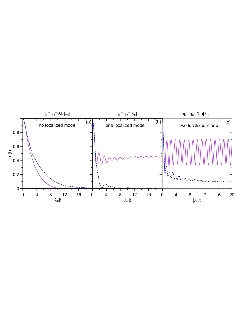
Figure 1: The absolute value of time-dependent spectral Green function $|u(t)|$ at different coupling ratios (a) $\eta_{L}=\eta_{R}=0.5|\lambda_{0}|$, (b) $\eta_{L}=\eta_{R}=1.0|\lambda_{0}|$, (c) $\eta_{L}=\eta_{R}=1.5|\lambda_{0}|$ with zero bias $eV_{SD}=\mu_{L}-\mu_{R}=U_{L}-U_{R}=0$ (magenta solid line) and a finite bias $eV_{SD}=\mu_{L}-\mu_{R}=U_{L}-U_{R}=3|\lambda_{0}|$ (navy blue dash line). The energy level of the quantum dot $\varepsilon_{c}=3|\lambda_{0}|$, and the band center of the two leads $\epsilon_{0}=2.5|\lambda_{0}|$. For the unbiased case, $\mu_{L}=\mu_{R}=2.5|\lambda_{0}|$, and $U_{L}=U_{R}=1.5|\lambda_{0}|$. For the biased case, $\mu_{L}=4|\lambda_{0}|$, $\mu_{R}=|\lambda_{0}|$, $U_{L}=3|\lambda_{0}|$, and $U_{R}=0$. We take $t_{0}=0$

The above different dissipation dynamics in the biased and unbiased cases will deeply change the transient and steady-state electron occupation in the dot and also the transport current. Fig. 2 shows the electron occupation in the dot and the transient transport current $I_{L}(t)=I_{R}(t)$ in the unbiased case for the partitioned and partition-free schemes. The partition-free system is initially at equilibrium so that the dot contains a fraction of an electron, while the dot is initially empty in the partitioned scheme. One can see that the effect of the initial correlations vanish in the long-time limit when there is no localized bound state. The steady-state electron occupation is the same for the partition-free and partitioned schemes. However, when one localized bound state appears, the electron occupation in the dot oscillates in time for both the partitioned and partition-free schemes, and approaches to different steady-state values. This indicates that the initial correlations can affect on the density matrix of the dot both in the transient and steady-state regimes due to the existence of localized bound state. When two localized bound states occur, it will generate an new oscillation with the frequency being the energy difference of the two localized bound states for the electron occupation and this oscillation will be maintained even in the steady state,Stef07195115 where the initial-correlation dependence becomes more significant, as shown in Fig. 2(c) for the electron occupation. The corresponding transient transport current for the partition-free and partitioned schemes approach to the same value in a every short time scale regardless whether the localized bound states exist or not. The steady-state current approaches to zero if there is no localized bound state. The current will also oscillate slightly when one localized bound state occurs and approaches to zero in the steady state. When both localized bound states appear, the current will keep oscillations around zero forever.Stef07195115 However, the initial-correlations dependence in the transport current is not as significant as in the electron occupation in both the transient and in the steady-state regimes, and even can be ignored in the steady-state limit, as shown in Fig. 2.

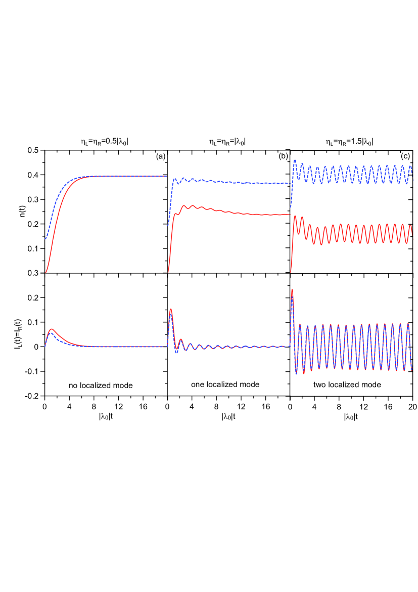
Figure 2: The transient electron occupation of the dot and the transient transport current for the unbiased case at different coupling ratios (a) $\eta_{L}=\eta_{R}=0.5|\lambda_{0}|$, (b) $\eta_{L}=\eta_{R}=|\lambda_{0}|$, (c) $\eta_{L}=\eta_{R}=1.5|\lambda_{0}|$ for the partition-free (blue-dash line) and partitioned (red solid line) schemes. The energy level of the quantum dot $\varepsilon_{c}=3|\lambda_{0}|$, the band center of the two leads $\epsilon_{0}=2.5|\lambda_{0}|$. For the partitioned scheme the leads are prepared at $\mu_{L}=\mu_{R}=2.5|\lambda_{0}|$, and $k_{B}T_{L}=k_{B}T_{R}=3|\lambda_{0}|$. For the partition-free scheme, the system is initially at equilibrium with $\mu=|\lambda_{0}|$ and $k_{B}T=3|\lambda_{0}|$. The applied bias voltage $U_{L}=U_{R}=1.5|\lambda_{0}|$ after $t_{0}=0$.

The time evolution of the electron occupation in the dot and the transient transport current for both the partitioned and the partition-free schemes for the biased case are shown in Fig. 3. Compare Fig. 2 with Fig. 3, one can find that the applied bias restrains most of the oscillation behavior in the electron occupation as well as in the transport current, except for the very beginning of the transient regime. Also, regardless of the existence of localized bound states, the electron occupation and also the transport current all approach to a steady-state value other than zero due to the non-zero bias. In other words, the localized bound state has a less effect on the electron occupation and the transport current when a bias is applied. This is because, as we have pointed out in the discussion of Fig.1(c), the applied bias can reduce significantly the amplitude of one of the localized bound states, which suppress the oscillation of the transport electrons between two localized bound states. However, the remaining localized bound state will result in a small different steady-state values for partition-free and partitioned schemes only in the electron occupation. The corresponding transient current flow through the left and right leads are quite different when a bias voltage is applied. In particular, the transient transport current in the right lead is positive in the beginning for the partitioned scheme because the dot is initially empty, and it approaches to a negative steady-state value in both schemes. But the steady-state current is almost independent of the initial correlations as shown in the inset graphs in Fig. 3. These result shows that the initial correlation effects are not so significant in the steady-state transport current in comparison with the electron occupation.

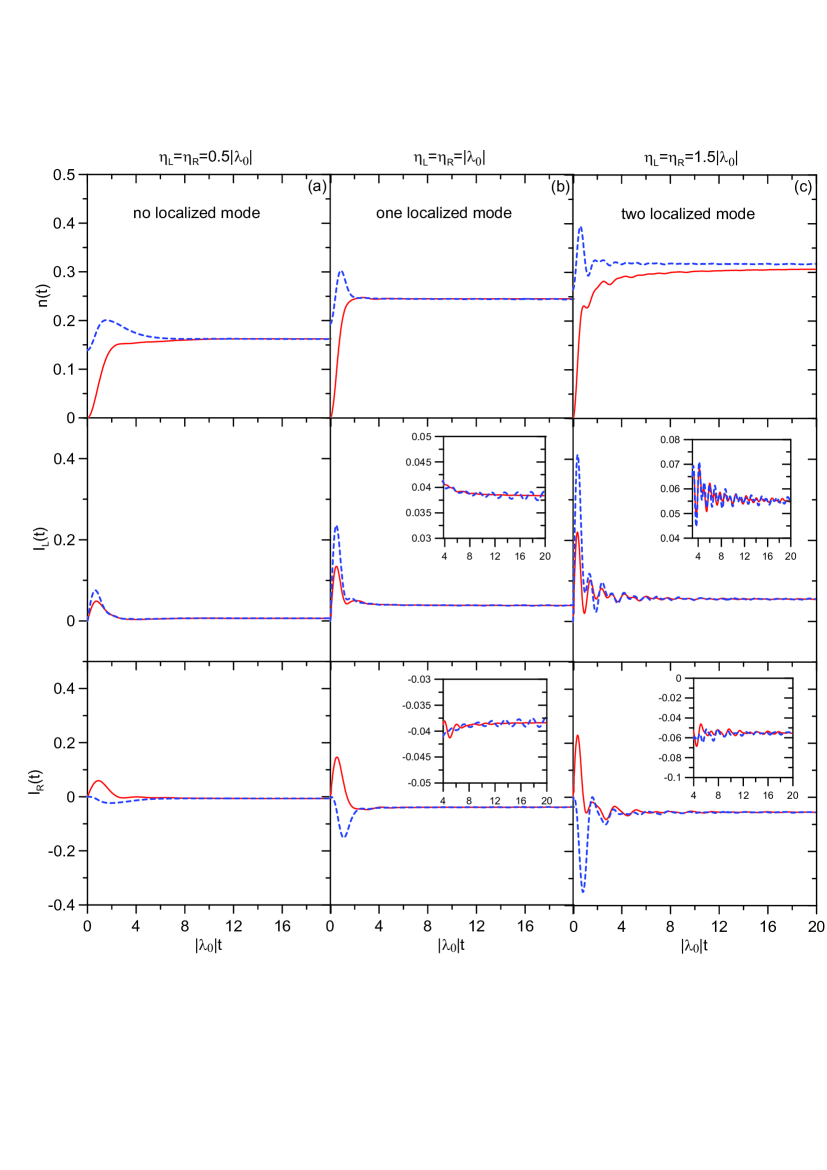
Figure 3: The transient electron occupation of the dot and the transient transport current for the biased case at different coupling ratios (a) $\eta_{L}=\eta_{R}=0.5|\lambda_{0}|$, (b) $\eta_{L}=\eta_{R}=|\lambda_{0}|$, (c) $\eta_{L}=\eta_{R}=1.5|\lambda_{0}|$ for the partition-free (blue-dash line) and partitioned (red solid line) schemes. The energy level of the quantum dot $\varepsilon_{c}=3|\lambda_{0}|$, the band center of the two leads $\epsilon_{0}=2.5|\lambda_{0}|$. For the partitioned scheme the leads are prepared at $\mu_{L}=4|\lambda_{0}|$, $\mu_{R}=|\lambda_{0}|$, and $k_{B}T_{L}=k_{B}T_{R}=3|\lambda_{0}|$. For the partition-free scheme, the system is initially at equilibrium with $\mu=|\lambda_{0}|$ and $k_{B}T=3|\lambda_{0}|$. The applied bias voltage $U_{L}=3|\lambda_{0}|$ and $U_{R}=0$ after $t_{0}=0$.

In the end, as a self-consistent check, we consider the case $U_{L}=U_{R}=0$. For the partition-free scheme, the system should stay in equilibrium. Our result is given in Fig. 4, which is expected. For the partitioned scheme, because of the appearance of two localized bound states, the electron occupation in the dot will keep oscillation around a steady-state value, and the system would never reach to equilibrium with the leads. Also, the current continuously oscillates with time around zero value. These results agree with the results obtained in Ref. [Stef07195115, ] and Ref. [Dhar06085119, ], in which one consider the effect of localized bound state in quantum transport for partition-free and partitioned schemes, respectively. In fact, these results also agree with the fact that Anderson pointed out in Anderson localization,Anderson namely, the system cannot approach to equilibrium when localized bound states occur.

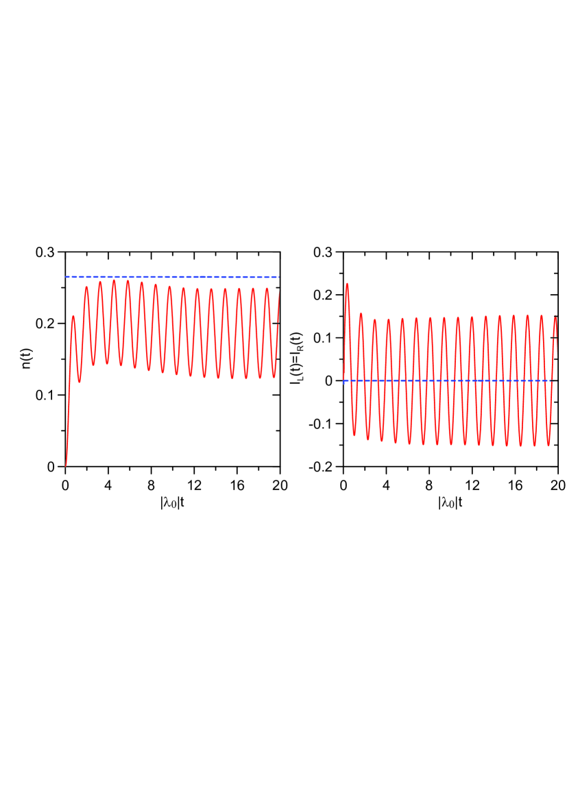
Figure 4: The transient electron occupation $n(t)$ and the transient transport current $I_{\alpha}(t)$ at the coupling ratio $\eta_{L}=\eta_{R}=1.5|\lambda_{0}|$ with no energy shift ($U_{L}=U_{R}=0$) for the partition-free (blue dash line) and partitioned system (red solid line). Other parameters are $\mu=\mu_{L}=\mu_{R}=|\lambda_{0}|$ and $k_{B}T=k_{B}T_{L}=k_{B}T_{R}=|\lambda_{0}|$

IV Summary and Discussion

In summary, we investigate the transport dynamics of nanostructured devices in the presence of initial system-lead and lead-lead correlations. By deriving the exact master equation through the extended quantum Langvein equation, the effect of initial correlations is explicitly built into the fluctuation coefficients in the master equation. The transient transport current incorporating with initial correlations is deduced from the master equation. Our transient transport theory based on master equation approach derived in this paper is suitable for arbitrary initial system-lead correlated state.

In application, we consider two initial states that are commonly discussed in the literatures, one is the partition-free scheme in which the initial correlations is presented explicitly. The other one is the partitioned scheme in which there is no initial correlations. The two schemes show the same steady-state behavior in the small system-lead coupling regime. When the coupling between the dot and the leads gets strong, localized bound states will appear, and these two schemes give some different results both in the transient regime and in the steady-state limit. It shows that the initial correlation effects can not be ignored if the localized bound states exist. Besides, when the localized bound states occur, the device system can not approach to equilibrium with the leads, and the initial correlation effects become more significant. These initial correlation effects accompanied by the localized bound state could be restrained by applying a finite bias voltage. Indeed, we find that a finite bias can suppress the oscillation behavior in the electron occupation and in the transport current induced by the simultaneous existence of two localized bound states. Compare with electron occupation in the dot, the steady-state current is insensitive to the initial states, so the results are not so distinguishable between the partitioned and the partition-free schemes. Nevertheless, the transport currents are quite different in the transient regime in these two schemes when the bias is applied. Although we only consider a noninteracting nanostructure as a model in the detailed exploration of the initial correlation effects, it is not difficult to extend to include electron-electron interactions in our theory because the coefficients of the master equation are expressed in terms of the nonequilibrium Green functions which can at least perturbatively or numerically handle the effect of electron-electron interactions. We leave this problem for further investigation.

References

• (1) H. Haug and A. P. Jauho, Quantum Kinetics in Transport and Optics of Semiconductors (Springer Series in Solid-State Sciences Vol. 123, 2008).
• (2) N. S. Wingreen, A. P. Jauho and Y. Meir, Phys. Rev. B 48, 8487(1993); idib. 50, 5528(1994).
• (3) Y. M. Blanter, and M. Büttiker, Phys. Rep 336, 1-166 (2000).
• (4) Y. Imry, Introduction to Mesoscopic Physics, (2nd Ed. Oxford, 2002).
• (5) S. Datta, Electronic Transport in Mesoscopic Systems(Cambridge, 1995).
• (6) J. Schwinger, J. Math. Phys. 2, 407 (1961); L. V. Keldysh, Sov. Phys. JETP 20, 1018 (1965).
• (7) L.P. Kadanoff and G. Baym, Quantum Statistical Mechanics(Benjamin, New York, 1962)
• (8) G. D. Mahan, Many Particle Physics (Plenum, New York, 1990), 2nd ed.
• (9) M. Büttiker, Phys. Rev. B 46, 12485 (1992).
• (10) Y. Meir, and N. S. Wingreen, Phys. Rev. Lett. 68, 2512(1992).
• (11) W. Lu, Z. Ji, L. Pfeiffer, K. W. West, and A. J. Rimberg, Nature (London) 423, 422 (2003).
• (12) J. Bylander, T. Duty, and P. Delsing, Nature (London) 434, 361 (2005)
• (13) S. Gustavsson, I. Shorubalko, R. Leturcq, S. Schön, and K. Ensslin, Appl. Phys. Lett. 92, 152101 (2008).
• (14) H. Schoeller and G. Schön, Phys. Rev. B 50, 18436 (1994).
• (15) S. A. Gurvitz and Ya. S. Prager, Phys. Rev. B 53, 19532 (1996).
• (16) X. Q. Li, J. Luo, Y. G. Yang, P. Cui, and Y. J. Yan, Phys. Rev. B 71, 205304 (2005).
• (17) J. S. Jin, X. Zheng, and Y. J. Yan, J. Chem. Phys. 128, 234703 (2008).
• (18) M. W. -Y. Tu and W. -M. Zhang, Phys. Rev. B 78, 235311 (2008); M. W. -Y. Tu, M.-T. Lee, and W. -M. Zhang, Quantum Inf. Processing (Springer) 8, 631 (2009).
• (19) J. S. Jin, M. W. -Y. Tu, W. -M. Zhang, and Y. J. Yan, New J. Phys. 12, 083013 (2010).
• (20) W. M. Zhang, P. Y. Lo, H. N. Xiong, M. W. Y. Tu, and F. Nori, Phys. Rev. Lett. 109, 170402 (2012).
• (21) M. W.-Y. Tu, W.-M. Zhang, J. S. Jin, O. Entin-Wohlman, and A. Aharony, Phys. Rev. B 86, 115453 (2012); M. W.-Y. Tu, A. Aharony, W.-M. Zhang, and O. Entin-Wohlman, Phys. Rev. B 90, 165422 (2014).
• (22) M. Moskalets and M. Büttiker, Phys. Rev. B 69, 205316 (2004).
• (23) M. Cini, Phys. Rev. B 22, 5887 (1980).
• (24) A. Dhar and D. Sen, Phys. Rev. B 73, 085119 (2006).
• (25) G. Stefanucci and C.-O. Almbladh, Phys. Rev. B 69, 195318 (2004).
• (26) G. Stefanucci, Phys. Rev. B 75, 195115 (2007).
• (27) J. Taylor, H. Guo, and J. Wang, Phys. Rev. B 63, 245407 (2001).
• (28) P. Pomorski, L. Pastewka, C. Roland, H. Guo, and J. Wang, Phys. Rev. B 69, 115418 (2004).
• (29) V. Vettchinkina, A. Kartsev, D. Karlsson, and C. Verdozzi, Phys. Rev. B 87, 115117 (2013).
• (30) P. W. Anderson, Phys. Rev. 109, 1492 (1958).
• (31) R. P. Feynman and F. L. Vernon, Ann. Phys. 24, 118 (1963).
• (32) P. Y. Yang, C. Y. Lin, and W. M. Zhang, Phys. Rev. B 89, 115411 (2014).
• (33) A. Schiller and S. Hershfield, Phys, Rev. B 58, 14978 (1998).