Linear interpolation method in ensemble Kohn–Sham and range-separated density-functional approximations for excited states

Abstract

Gross–Oliveira–Kohn density functional theory (GOK-DFT) for ensembles is in principle very attractive, but has been hard to use in practice. A novel, practical model based on GOK-DFT for the calculation of electronic excitation energies is discussed. The new model relies on two modifications of GOK-DFT: use of range separation and use of the slope of the linearly-interpolated ensemble energy, rather than orbital energies. The range-separated approach is appealing as it enables the rigorous formulation of a multi-determinant state-averaged DFT method. In the exact theory, the short-range density functional, that complements the long-range wavefunction-based ensemble energy contribution, should vary with the ensemble weights even when the density is held fixed. This weight dependence ensures that the range-separated ensemble energy varies linearly with the ensemble weights. When the (weight-independent) ground-state short-range exchange-correlation functional is used in this context, curvature appears thus leading to an approximate weight-dependent excitation energy. In order to obtain unambiguous approximate excitation energies, we propose to interpolate linearly the ensemble energy between equiensembles. It is shown that such a linear interpolation method (LIM) can be rationalized and that it effectively introduces weight dependence effects. As proof of principle, LIM has been applied to He, Be, H₂ in both equilibrium and stretched geometries as well as the stretched HeH⁺ molecule. Very promising results have been obtained for both single (including charge transfer) and double excitations with spin-independent short-range local and semi-local functionals. Even at the Kohn–Sham ensemble DFT level, that is recovered when the range-separation parameter is set to zero, LIM performs better than standard time-dependent DFT.

I Introduction

The standard approach for modeling excited states in the framework of density-functional theory (DFT) is the time-dependent (TD) linear response regime Casida and Huix-Rotllant (2012). Despite its success, due to its low computational cost and relatively good accuracy, standard TD-DFT still suffers from various deficiencies, one of them being the absence of multiple excitations in the spectrum. This is directly connected with the so-called adiabatic approximation that consists in using a frequency-independent exchange-correlation kernel in the linear response equations. In order to overcome such limitations, the combination of TD-DFT with density-matrix- Pernal (2012) or wavefunction-based Rebolini et al. (2013); Fromager et al. (2013); Hedegård et al. (2013) methods by means of range separation has been investigated recently.
In this work, we propose to explore a time-independent range-separated DFT approach for excited states that is based on ensembles Gross et al. (1988a, b). One of the motivation is the need for cheaper (in terms of computational cost) yet still reliable (in terms of accuracy) alternatives to standard second-order complete active space (CASPT2) Andersson et al. (1992) or N-electron valence state (NEVPT2) Angeli et al. (2001, 2002) perturbation theories for modeling, for example, photochemical processes Nikiforov et al. (2014); Filatov (2015). Ensemble range-separated DFT was initially formulated by Pastorczak et al. Pastorczak et al. (2013) The authors considered the particular case of Boltzmann ensemble weights. The latter were controlled by an effective temperature that can be used as a tunable parameter, in addition to the range-separation one. As shown in Ref. Franck and Fromager (2014), an exact adiabatic connection formula can be derived for the complementary short-range exchange-correlation energy of an ensemble. Exactly like in Kohn–Sham (KS) ensemble DFT Gross et al. (1988b); Yang et al. (2014); Pribram-Jones et al. (2014), that is also referred to as Gross–Oliveira–Kohn DFT (GOK-DFT), the variation of the short-range exchange-correlation density functional with the ensemble weights plays a crucial role in the calculation of excitation energies Franck and Fromager (2014). So far, short-range density-functional approximations have been developed only for the ground state, not for ensembles. Consequently, an approximate (weight-independent) ground-state functional was used in Ref. Pastorczak et al. (2013).
The weight dependence of the range-separated ensemble energy and the ambiguity in the definition of an approximate excitation energy, that may become weight-dependent when approximate functionals are used, will be analyzed analytically and numerically in this work. By analogy with the fundamental gap problem Stein et al. (2012), a simple and general linear interpolation method is proposed and interpreted for the purpose of defining unambiguously approximate weight-independent excitation energies. The method becomes exact if exact functionals and wavefunctions are used. The paper is organized as follows: After a brief introduction to ground-state range-separated DFT in Sec. II.1, GOK-DFT is presented in Sec. II.2 and its exact range-separated extension is formulated in Sec. II.3. The weight-independent density-functional approximation is then discussed in detail for a two-state ensemble. The linear interpolation method is introduced in Sec. II.4 and rationalized in Sec. II.5. The particular case of an approximate range-separated ensemble energy that is quadratic in the ensemble weight is then treated in Sec. II.6. Comparison is made with Ref. Pastorczak et al. (2013) and time-dependent adiabatic linear response theory in Sec. II.7. A generalization to higher excitations is then given in Sec. II.8. After the computational details in Sec. III, results obtained for He, Be, H₂ and HeH⁺ are presented and discussed in Sec. IV. We conclude this work with a summary in Sec. V.

II Theory

II.1 Range-separated density-functional theory for the ground state

According to the Hohenberg–Kohn (HK) theorem Hohenberg and Kohn (1964), the exact ground-state energy of an electronic system can be obtained variationally as follows,

$$E_{0} = \underset{n}{\rm min}\Big{\{}F[n]+\int{\rm d}{\bf r}\,v_{\rm ne}({\bf r})\,n({\bf r})\Big{\}},$$ (1)

where $v_{\rm ne}({\bf r})$ is the nuclear potential and the minimization is performed over electron densities $n({\bf r})$ that integrate to a fixed number $N$ of electrons. The universal Levy–Lieb (LL) functional Lieb (1983) equals

$$F[n]=\underset{\Psi\rightarrow n}{\rm min}\langle\Psi|\hat{T}+{\hat{W}_{\rm ee}}|\Psi\rangle,$$ (2)

where $\hat{T}$ and $\hat{W}_{\rm ee}\equiv\sum^{N}_{i<j}1/r_{ij}$ are the kinetic energy and regular two-electron repulsion operators, respectively. Following Savin Savin (1996), we consider the decomposition of the latter into long- and short-range contributions,

$${1}/{r_{12}} = w^{\rm lr,\mu}_{\rm ee}(r_{12})+w^{\rm sr,\mu}_{\rm ee}(r_{12}),$$

$$w^{\rm lr,\mu}_{\rm ee}(r_{12}) = {\rm erf}(\mu r_{12})/r_{12},$$ (3)

where $\rm erf$ is the error function and $\mu$ is a parameter in $[0,+\infty[$ that controls the range separation, thus leading to the partitioning

$$F[n]=F^{\rm lr,\mu}[n]+{E}^{\rm sr,\mu}_{\rm Hxc}[n],$$ (4)

with

$$F^{\rm lr,\mu}[n]=\underset{\Psi\rightarrow n}{\rm min}\langle\Psi|\hat{T}+{\hat{W}^{\rm lr,\mu}_{\rm ee}}|\Psi\rangle,$$ (5)

and $\hat{W}^{\rm lr,\mu}_{\rm ee}\equiv\sum^{N}_{i<j}w^{\rm lr,\mu}_{\rm ee}(r_{ij})$. The complementary $\mu$-dependent short-range density-functional energy ${E}^{\rm sr,\mu}_{\rm Hxc}[n]$ can be decomposed into Hartree (H) and exchange-correlation (xc) terms, in analogy with conventional KS-DFT,

$${E}^{\rm sr,\mu}_{\rm Hxc}[n] = {E}^{\rm sr,\mu}_{\rm H}[n]+{E}^{\rm sr,\mu}_{\rm xc}[n],$$

$$E^{{\rm sr},\mu}_{\rm H}[n] = \frac{1}{2}\int\int{\rm d}{\mathbf{r}}{\rm d}{\mathbf{r^{\prime}}}n(\mathbf{r})n(\mathbf{r^{\prime}})w^{\rm sr,\mu}_{\rm ee}\left(|{\bf r}-{\bf r^{\prime}}|\right).$$ (6)

Inserting Eq. (4) into Eq. (1) leads to the exact expression

$$E_{0} = {\displaystyle\underset{\Psi}{\rm min}\left\{\langle\Psi|\hat{T}+\hat{W}^{\rm lr,\mu}_{\rm ee}+\hat{V}_{\rm ne}|\Psi\rangle+E^{\rm sr,\mu}_{\rm Hxc}[n_{\Psi}]\right\}}$$ (7)

$$= \langle\Psi_{0}^{\mu}|\hat{T}+\hat{W}^{\rm lr,\mu}_{\rm ee}+\hat{V}_{\rm ne}|\Psi_{0}^{\mu}\rangle+E^{\rm sr,\mu}_{\rm Hxc}[n_{\Psi_{0}^{\mu}}],$$

where $\hat{V}_{\rm ne}=\int{\rm d}{\bf r}\,v_{\rm ne}({\bf r})\,\hat{n}({\bf r})$ and $\hat{n}(\mathbf{r})$ is the density operator. The electron density obtained from the trial wavefunction $\Psi$ is denoted $n_{\Psi}$. The exact minimizing wavefunction $\Psi_{0}^{\mu}$ in Eq. (7) has the same density $n^{0}$ as the physical fully-interacting ground-state wavefunction $\Psi_{0}$ and it fulfils the following self-consistent equation:

$$\hat{H}^{\mu}[n_{\Psi_{0}^{\mu}}]|{\Psi}^{\mu}_{0}\rangle={\mathcal{E}}^{\mu}_{0}|{\Psi}^{\mu}_{0}\rangle,$$ (8)

where

$$\hat{H}^{\mu}[n]=\hat{T}+\hat{W}^{\rm lr,\mu}_{\rm ee}+\hat{V}_{\rm ne}+\int{\rm d}\mathbf{r}\dfrac{\delta E^{{\rm sr,\mu}}_{\rm Hxc}[n]}{\delta n(\mathbf{r})}\hat{n}(\mathbf{r}).$$ (9)

It is readily seen from Eqs. (II.1) and (8) that the KS and Schrödinger equations are recovered in the limit of $\mu=0$ and $\mu\rightarrow+\infty$, respectively. An exact combination of wavefunction theory with KS-DFT is obtained in the range of $0<\mu<+\infty$.
In order to perform practical range-separated DFT calculations, local and semi-local short-range density functionals have been developed in recent years Toulouse et al. (2004a, b); Goll et al. (2005, 2009). In addition, various wavefunction-theory-based methods have been adapted to this context in order to describe the long-range interaction: Hartree–Fock (HF) Ángyán et al. (2005); Fromager et al. (2007), second-order Møller-Plesset (MP2) Ángyán et al. (2005); Fromager and Jensen (2008); Ángyán (2008), the random-phase approximation (RPA) Toulouse et al. (2009); Janesko et al. (2009), configuration interaction (CI) Leininger et al. (1997); Pollet et al. (2002), coupled-cluster (CC) Goll et al. (2005), the multi-configurational self-consistent field (MCSCF) Fromager et al. (2007), NEVPT2 Fromager et al. (2010), one-electron reduced density-matrix-functional theory Rohr et al. (2010) (RDMFT) and the density matrix renormalization group method Hedegård et al. (2015) (DMRG). In this work, CI will be used. The orbitals, referred to as HF short-range DFT (HF-srDFT) orbitals in the following, are generated by restricting the minimization on the first line of Eq. (7) to single determinantal wavefunctions. Note that, when $\mu=0$, the HF-srDFT orbitals reduce to the conventional KS ones.
Finally, in connection with the description of excited states, let us mention that the exact auxiliary excited states $\{\Psi_{i}^{\mu}\}_{i>0}$ that fulfil the eigenvalue equation,

$$\hat{H}^{\mu}[n_{\Psi_{0}^{\mu}}]|{\Psi}^{\mu}_{i}\rangle={\mathcal{E}}^{\mu}_{i}|{\Psi}^{\mu}_{i}\rangle,$$ (10)

can be used as starting points for reaching the physical excitation energies by means of extrapolation techniques Savin (2014); Rebolini et al. (2014, 2015a), perturbation theory Rebolini et al. (2015b), time-dependent linear response theory Fromager et al. (2013); Hedegård et al. (2013) or ensemble range-separated DFT Pastorczak et al. (2013); Franck and Fromager (2014), as discussed further in the following.

II.2 Ensemble density-functional theory for excited states

According to the GOK variational principle Gross et al. (1988a), that generalizes the seminal work of Theophilou Theophilou (1979) on equiensembles, the following inequality

$$E^{\mathbf{w}}\leq{\rm Tr}\left[\hat{\Gamma}^{\mathbf{w}}\hat{H}\right],$$ (11)

where $\hat{H}=\hat{T}+\hat{W}_{\rm ee}+\hat{V}_{\rm ne}$ and ${\rm Tr}$ denotes the trace, is fulfilled for any ensemble characterized by a set of weights $\mathbf{w}\equiv(w_{0},w_{1},\ldots,w_{M-1})$ with $w_{0}\geq w_{1}\geq\ldots\geq w_{M-1}>0$ and a set of $M$ orthonormal trial wavefunctions $\{\overline{\Psi}_{k}\}_{0\leq k\leq M-1}$ from which a trial density matrix can be constructed:

$$\hat{\Gamma}^{\mathbf{w}}=\sum^{M-1}_{k=0}w_{k}|\overline{\Psi}_{k}\rangle\langle\overline{\Psi}_{k}|.$$ (12)

The lower bound in Eq. (11) is the exact ensemble energy

$$E^{\mathbf{w}}=\sum_{k=0}^{M-1}w_{k}\langle\Psi_{k}|\hat{H}|\Psi_{k}\rangle=\sum_{k=0}^{M-1}w_{k}E_{k},$$ (13)

where $\Psi_{k}$ is the exact $k$th eigenfunction of $\hat{H}$ and $E_{0}\leq E_{1}\leq\ldots\leq E_{M-1}$. In the following, the ensemble will always contain complete sets of degenerate states (referred to as ”multiplets” in Ref. Gross et al. (1988b)). An important consequence of the GOK principle is that the HK theorem can be extended to ensembles of ground and excited states Gross et al. (1988b), thus leading to the exact variational expression for the ensemble energy,

$$E^{\mathbf{w}}=\underset{n}{\rm min}\left\{F^{\mathbf{w}}[n]+\int{\rm d}\mathbf{r}\;v_{\rm ne}(\mathbf{r})n(\mathbf{r})\right\},$$ (14)

where the universal LL ensemble functional is defined as follows,

$$F^{\mathbf{w}}[n]=\underset{\hat{\Gamma}^{\mathbf{w}}\rightarrow n}{\rm min}\left\{{\rm Tr}\left[\hat{\Gamma}^{\mathbf{w}}(\hat{T}+\hat{W}_{\rm ee})\right]\right\}.$$ (15)

The minimization in Eq. (15) is restricted to ensemble density matrices with the ensemble density $n$:

$${\rm Tr}\left[\hat{\Gamma}^{\mathbf{w}}\hat{n}(\mathbf{r})\right]=n_{\hat{\Gamma}^{\mathbf{w}}}(\mathbf{r})=n(\mathbf{r}).$$ (16)

Note that, in the following, we will use the convention $\sum_{k=0}^{M-1}w_{k}=1$ so that the ensemble density integrates to the number of electrons $N$. The minimizing density in Eq. (14) is the exact ensemble density of the physical system $n^{\mathbf{w}}(\mathbf{r})=\sum_{k=0}^{M-1}w_{k}\,n_{\Psi_{k}}(\mathbf{r})$.

In standard ensemble DFT Gross et al. (1988b), that is referred to as GOK-DFT in the following, the KS partitioning of the LL functional is used,

$$F^{\mathbf{w}}[n]=T_{\rm s}^{\mathbf{w}}[n]+E_{\rm Hxc}^{\mathbf{w}}[n],$$ (17)

where the non-interacting ensemble kinetic energy is defined as

$$T_{\rm s}^{\mathbf{w}}[n]=\underset{\hat{\Gamma}^{\mathbf{w}}\rightarrow n}{\rm min}\left\{{\rm Tr}\left[\hat{\Gamma}^{\mathbf{w}}\hat{T}\right]\right\},$$ (18)

and $E_{\rm Hxc}^{\mathbf{w}}[n]$ is the $\mathbf{w}$-dependent Hxc functional for the ensemble, thus leading to the exact ensemble energy expression, according to Eq. (14),

$$E^{\mathbf{w}}=\underset{\hat{\Gamma}^{\mathbf{w}}}{\rm min}\left\{{\rm Tr}\left[\hat{\Gamma}^{\mathbf{w}}(\hat{T}+\hat{V}_{\rm ne})\right]+E_{\rm Hxc}^{\mathbf{w}}[n_{\hat{\Gamma}^{\mathbf{w}}}]\right\}.$$ (19)

The minimizing GOK density matrix,

$$\hat{\Gamma}_{\rm s}^{\mathbf{w}}=\sum_{k=0}^{M-1}w_{k}|\Phi^{\mathbf{w}}_{k}\rangle\langle\Phi^{\mathbf{w}}_{k}|,$$ (20)

reproduces the exact ensemble density of the physical system,

$$n_{\hat{\Gamma}_{\rm s}^{\mathbf{w}}}(\mathbf{r})=n^{\mathbf{w}}(\mathbf{r}),$$ (21)

and it fulfils the stationarity condition $\delta\mathcal{L}^{\mathbf{w}}[\hat{\Gamma}_{\rm s}^{\mathbf{w}}]=0$ where

$$\mathcal{L}^{\mathbf{w}}[\hat{\Gamma}^{\mathbf{w}}] = {\rm Tr}\left[\hat{\Gamma}^{\mathbf{w}}(\hat{T}+\hat{V}_{\rm ne})\right]+E_{\rm Hxc}^{\mathbf{w}}[n_{\hat{\Gamma}^{\mathbf{w}}}]$$ (22)

$$+\sum_{k=0}^{M-1}w_{k}\mathcal{E}^{\mathbf{w}}_{k}\Big{(}1-\langle\overline{\Psi}_{k}|\overline{\Psi}_{k}\rangle\Big{)}.$$

The coefficients $\mathcal{E}^{\mathbf{w}}_{k}$ are Lagrange multipliers associated with the normalization of the trial wavefunctions $\overline{\Psi}_{k}$ from which the density matrix is built. Considering variations $\overline{\Psi}_{k}\rightarrow\overline{\Psi}_{k}+\delta\overline{\Psi}_{k}$ for each individual states separately leads to the self-consistent GOK equations Gross et al. (1988b):

$$\Bigg{(}\hat{T}+\hat{V}_{\rm ne}+\int{\rm d}\mathbf{r}\dfrac{\delta E_{\rm Hxc}^{\mathbf{w}}[n_{\hat{\Gamma}_{\rm s}^{\mathbf{w}}}]}{\delta n(\mathbf{r})}\hat{n}(\mathbf{r})\Bigg{)}|\Phi^{\mathbf{w}}_{k}\rangle$$

$$=\mathcal{E}^{\mathbf{w}}_{k}|\Phi^{\mathbf{w}}_{k}\rangle,\hskip 5.69046pt0\leq k\leq M-1.$$ (23)

II.3 Range-separated ensemble density-functional theory

In analogy with ground-state range-separated DFT, the LL ensemble functional in Eq. (15) can be range-separated as follows Pastorczak et al. (2013); Franck and Fromager (2014),

$$F^{\mathbf{w}}[n]=F^{\rm lr,\mu,\mathbf{w}}[n]+{E}^{\rm sr,\mu,\mathbf{w}}_{\rm Hxc}[n],$$ (24)

where

$$F^{\rm lr,\mu,\mathbf{w}}[n]=\underset{\hat{\Gamma}^{\mathbf{w}}\rightarrow n}{\rm min}\left\{{\rm Tr}\left[\hat{\Gamma}^{\mathbf{w}}(\hat{T}+\hat{W}^{\rm lr,\mu}_{\rm ee})\right]\right\}.$$ (25)

In the following, the short-range ensemble functional will be partitioned into $\mathbf{w}$-independent Hartree and $\mathbf{w}$-dependent exchange-correlation terms,

$${E}^{\rm sr,\mu,\mathbf{w}}_{\rm Hxc}[n] = {E}^{\rm sr,\mu}_{\rm H}[n]+{E}^{\rm sr,\mu,\mathbf{w}}_{\rm xc}[n].$$ (26)

Note that the decomposition is arbitrary and can be exact or not, depending on the short-range exchange-correlation functional used. In practical calculations, local and semi-local exchange-correlation functionals may not remove the so-called ”ghost interactions” Gidopoulos et al. (2002); Pastorczak and Pernal (2014) that are included into the short-range Hartree term. Such interactions are fictitious and unwanted. Their detailed analysis, in the context of range-separated ensemble DFT, is currently in progress and will be presented in a separate work.
Combining Eq. (14) with Eq. (24) leads to the exact range-separated ensemble energy expression

$$E^{\mathbf{w}}=\underset{\hat{\Gamma}^{\mathbf{w}}}{\rm min}\Big{\{} {\rm Tr}\left[\hat{\Gamma}^{\mathbf{w}}(\hat{T}+\hat{W}^{\rm lr,\mu}_{\rm ee}+\hat{V}_{\rm ne})\right]$$ (27)

$$+E_{\rm Hxc}^{\rm sr,\mu,\mathbf{w}}[n_{\hat{\Gamma}^{\mathbf{w}}}]\Big{\}}.$$

The minimizing long-range-interacting ensemble density matrix $\hat{\Gamma}^{\mu,\mathbf{w}}=\sum_{k=0}^{M-1}w_{k}|\Psi^{\mu,\mathbf{w}}_{k}\rangle\langle\Psi^{\mu,\mathbf{w}}_{k}|$ reproduces the physical ensemble density,

$$n_{\hat{\Gamma}^{\mu,\mathbf{w}}}(\mathbf{r})=n^{\mathbf{w}}(\mathbf{r}),$$ (28)

and, by analogy with Eq. (22), we conclude that it should fulfill the self-consistent equation

$$\Bigg{(}\hat{T}+\hat{W}^{\rm lr,\mu}_{\rm ee}+\hat{V}_{\rm ne}+\int{\rm d}\mathbf{r}\dfrac{\delta E_{\rm Hxc}^{\rm sr,\mu,\mathbf{w}}[n_{\hat{\Gamma}^{\mu,\mathbf{w}}}]}{\delta n(\mathbf{r})}\hat{n}(\mathbf{r})\Bigg{)}|\Psi^{\mu,\mathbf{w}}_{k}\rangle$$

$$=\mathcal{E}^{\mu,\mathbf{w}}_{k}|\Psi^{\mu,\mathbf{w}}_{k}\rangle,\hskip 5.69046pt0\leq k\leq M-1.$$ (29)

Note that the Schrödinger and GOK-DFT equations are recovered for $\mu\rightarrow+\infty$ and $\mu=0$, respectively.

In the rest of this work we will mainly focus on ensembles consisting of two non-degenerate states. In this case, the ensemble weights are simply equal to

$$w_{1}=w,\hskip 5.69046ptw_{0}=1-w,$$ (30)

where $0\leq w\leq 1/2$, and the exact ensemble energy is a linear function of $w$,

$$E^{w}=(1-w)E_{0}+w\,E_{1}.$$ (31)

Consequently, the first excitation energy $\omega=E_{1}-E_{0}$ can be written either as a first-order derivative,

$$\omega=\dfrac{{\rm d}E^{w}}{{\rm d}w},$$ (32)

or as the slope of the linear interpolation between $w=0$ and $w=1/2$,

$$\omega=2(E^{w=1/2}-E_{0}).$$ (33)

Let us stress that Eqs. (32) and (33) are equivalent in the exact theory. By using the decomposition (see Eqs. (27) and (28))

$$E^{w}=(1-w)\langle\Psi^{\mu,w}_{0}|\hat{T}+\hat{W}^{\rm lr,\mu}_{\rm ee}+\hat{V}_{\rm ne}|\Psi^{\mu,w}_{0}\rangle$$

$$+w\langle\Psi^{\mu,w}_{1}|\hat{T}+\hat{W}^{\rm lr,\mu}_{\rm ee}+\hat{V}_{\rm ne}|\Psi^{\mu,w}_{1}\rangle+E^{{\rm sr,\mu,}w}_{\rm Hxc}[n^{w}],$$ (34)

that can be rewritten in terms of the auxiliary long-range interacting energies as follows, according to Eq. (II.3),

$${E}^{w}=(1-w){\mathcal{E}}^{\mu,w}_{0}+w{\mathcal{E}}^{\mu,w}_{1}$$

$$-\int{\rm d}\mathbf{r}\dfrac{\delta E^{{\rm sr,\mu},w}_{\rm Hxc}[{n}^{w}]}{\delta n(\mathbf{r})}{n}^{w}(\mathbf{r})+E^{{\rm sr,\mu},w}_{\rm Hxc}[{n}^{w}],$$ (35)

where the physical ensemble density equals the auxiliary one (see Eq. (28)),

$$n^{w}(\mathbf{r})=(1-w)n_{\Psi^{\mu,w}_{0}}(\mathbf{r})+w\,n_{\Psi^{\mu,w}_{1}}(\mathbf{r}),$$ (36)

and by applying the Hellmann–Feynman theorem,

$$\dfrac{{\rm d}{\mathcal{E}}^{\mu,w}_{i}}{{\rm d}w}=\int{\rm d}\mathbf{r}\dfrac{\partial}{\partial w}\Bigg{(}\dfrac{\delta E^{{\rm sr,\mu},w}_{\rm Hxc}[{n}^{w}]}{\delta n(\mathbf{r})}\Bigg{)}{n}_{{\Psi}^{\mu,w}_{i}}(\mathbf{r}),$$ (37)

we finally recover from Eq. (32) the following expression for the first excitation energy Franck and Fromager (2014),

$$\omega = \mathcal{E}^{\mu,w}_{1}-\mathcal{E}^{\mu,w}_{0}+\left.\dfrac{\partial E^{{\rm sr,\mu,}w}_{\rm Hxc}[n]}{\partial w}\right|_{n=n^{w}}$$ (38)

$$= \Delta\mathcal{E}^{\mu,w}+\Delta_{\rm xc}^{\mu,w}.$$

It is readily seen from Eq. (38) that the auxiliary excitation energy $\Delta\mathcal{E}^{\mu,w}=\mathcal{E}^{\mu,w}_{1}-\mathcal{E}^{\mu,w}_{0}$ differs in principle from the physical one. They become equal when $\mu\rightarrow+\infty$. For finite $\mu$ values, the difference is simply expressed in terms of a derivative with respect to the ensemble weight $\Delta_{\rm xc}^{\mu,w}=\left.\partial E^{{\rm sr,\mu,}w}_{\rm xc}[n]/\partial w\right|_{n=n^{w}}$. Note that the Hartree term does not contribute to the second term on the right-hand side of Eq. (38) since it is, for a given density $n$, $w$-independent (see Eq. (26)). Interestingly, when $w\rightarrow 0$, an exact expression for the physical excitation energy is obtained in terms of the auxiliary one that is associated with the ground-state density (see Eq. (10)),

$$\omega = \mathcal{E}^{\mu}_{1}-\mathcal{E}^{\mu}_{0}+\left.\dfrac{\partial E^{{\rm sr,\mu,}w}_{\rm xc}[n^{0}]}{\partial w}\right|_{w=0}.$$ (39)

Note also that, when $\mu=0$ and the first excitation is a one-particle–one-hole excitation (single excitation), the GOK expression Gross et al. (1988b) is recovered from Eq. (38),

$$\omega=\Delta\epsilon^{w}+\Delta_{\rm xc}^{w},$$ (40)

where $\Delta\epsilon^{w}=\varepsilon^{w}_{1}-\varepsilon^{w}_{0}$ is the HOMO-LUMO gap for the non-interacting ensemble and $\Delta_{\rm xc}^{w}=\left.\partial E^{w}_{\rm xc}[n]/\partial w\right|_{n=n^{w}}$. In the $w\rightarrow 0$ limit, the exact excitation energy can be expressed in terms of the KS HOMO $\varepsilon_{0}$ and LUMO $\varepsilon_{1}$ energies as follows,

$$\omega=\varepsilon^{w\rightarrow 0}_{1}-\varepsilon_{0},$$ (41)

where $\varepsilon^{w\rightarrow 0}_{1}=\varepsilon_{1}+\Delta_{\rm xc}^{0}$. As shown analytically by Levy Levy (1995) and numerically by Yang et al. Yang et al. (2014), $\Delta_{\rm xc}^{0}$ corresponds to the jump in the exchange-correlation potential when moving from $w=0$ (ground state) to $w>0$ (ensemble of ground and excited states). This is known as the derivative discontinuity (DD) and should not be confused with the ground-state DD that is related to ionization energies and electron affinities, although there are distinct similarities at a formal level Kraisler and Kronik (2013, 2014); Gould and Toulouse (2014). Consequently, the quantity $\Delta_{\rm xc}^{\mu,w}$ introduced in Eq. (38) will be referred to in the following as short-range DD.

II.4 Weight-independent density-functional approximation and the linear interpolation method

Even though an exact adiabatic-connection-based expression exists for the short-range ensemble exchange-correlation functional (see Eq. (133) in Ref. Franck and Fromager (2014)), it has not been used yet for developing weight-dependent density-functional approximations. Let us stress that this is still a challenge also in the context of GOK-DFT Yang et al. (2014). A crude approximation simply consists in using the ground-state functional Pastorczak et al. (2013),

$$E^{{\rm sr,\mu,}w}_{\rm xc}[n]\rightarrow E^{{\rm sr,\mu}}_{\rm xc}[n],$$ (42)

thus leading to the approximate ensemble energy expression

$$\tilde{E}^{\mu,w}=(1-w)\langle\tilde{\Psi}^{\mu,w}_{0}|\hat{T}+\hat{W}^{\rm lr,\mu}_{\rm ee}+\hat{V}_{\rm ne}|\tilde{\Psi}^{\mu,w}_{0}\rangle$$

$$+w\langle\tilde{\Psi}^{\mu,w}_{1}|\hat{T}+\hat{W}^{\rm lr,\mu}_{\rm ee}+\hat{V}_{\rm ne}|\tilde{\Psi}^{\mu,w}_{1}\rangle+E^{{\rm sr,\mu}}_{\rm Hxc}[\tilde{n}^{\mu,w}],$$ (43)

that may depend on both $\mu$ and $w$, and where the approximate auxiliary ensemble density equals

$$\tilde{n}^{\mu,w}(\mathbf{r})=(1-w)n_{\tilde{\Psi}^{\mu,w}_{0}}(\mathbf{r})+w\,n_{\tilde{\Psi}^{\mu,w}_{1}}(\mathbf{r}),$$ (44)

with

$$\hat{H}^{\mu}[\tilde{n}^{\mu,w}]|\tilde{\Psi}^{\mu,w}_{i}\rangle=\tilde{\mathcal{E}}^{\mu,w}_{i}|\tilde{\Psi}^{\mu,w}_{i}\rangle,\hskip 8.5359pti=0,1.$$ (45)

In the following we refer to this approximation as weight-independent density-functional approximation (WIDFA). Note that, at the WIDFA level, the ground-state density-functional Hamiltonian $\hat{H}^{\mu}[n]$ (see Eq. (9)) is used. The auxiliary wavefunctions $\tilde{\Psi}^{\mu,w}_{i}$ associated with the bi-ensemble ($0<w\leq 1/2$) will therefore deviate from their ”ground-state” limits $\Psi^{\mu}_{i}$ ($w=0$) because of the ensemble density $\tilde{n}^{\mu,w}$ that is inserted into the short-range Hxc potential. Note that Eq. (45) should be solved self-consistently. Let us also stress that the ground-state short-range Hxc density-functional potential ${\delta E^{{\rm sr,\mu}}_{\rm Hxc}[n^{0}]}/{\delta n(\mathbf{r})}$ is recovered in the limit $w\rightarrow 0$, as readily seen from Eq. (45). In other words, the short-range DD is not modeled at the WIDFA level of approximation. Finally, the exact ($\mu$-independent) ground-state energy will still be recovered when $w\rightarrow 0$ if no approximation is introduced in the short-range exchange-correlation functional,

$$\tilde{E}^{\mu,0}=E_{0}.$$ (46)

Obviously, the exact ensemble energy will in general not be recovered for $w>0$. By rewriting the WIDFA ensemble energy as

$$\tilde{E}^{\mu,w}=(1-w)\tilde{\mathcal{E}}^{\mu,w}_{0}+w\tilde{\mathcal{E}}^{\mu,w}_{1}$$

$$-\int{\rm d}\mathbf{r}\dfrac{\delta E^{{\rm sr,\mu}}_{\rm Hxc}[\tilde{n}^{\mu,w}]}{\delta n(\mathbf{r})}\tilde{n}^{\mu,w}(\mathbf{r})+E^{{\rm sr,\mu}}_{\rm Hxc}[\tilde{n}^{\mu,w}],$$ (47)

and applying the Hellmann–Feynman theorem,

$$\dfrac{{\rm d}\tilde{\mathcal{E}}^{\mu,w}_{i}}{{\rm d}w}=\int{\rm d}\mathbf{r}\dfrac{\partial}{\partial w}\Bigg{(}\dfrac{\delta E^{{\rm sr,\mu}}_{\rm Hxc}[\tilde{n}^{\mu,w}]}{\delta n(\mathbf{r})}\Bigg{)}{n}_{\tilde{\Psi}^{\mu,w}_{i}}(\mathbf{r}),$$ (48)

we see that, within WIDFA, the first-order derivative of the ensemble energy reduces to the auxiliary excitation energy that is in principle $w$-dependent,

$$\dfrac{{\rm d}\tilde{E}^{\mu,w}}{{\rm d}w} = \tilde{\mathcal{E}}^{\mu,w}_{1}-\tilde{\mathcal{E}}^{\mu,w}_{0}=\Delta\tilde{\mathcal{E}}^{\mu,w}.$$ (49)

Therefore, in practical calculations, the WIDFA ensemble energy may not be strictly linear in $w$, as illustrated for He in Fig. 1. In the same spirit as Ref. Stein et al. (2012), we propose to restore the linearity by means of a simple linear interpolation between the ground state ($w=0$) and the equiensemble ($w=1/2$),

$$\overline{E}^{\mu,w}=E_{0}+2w(\tilde{E}^{\mu,1/2}-E_{0}).$$ (50)

This approach, that will be rationalized in Sec. II.5, is referred to as linear interpolation method (LIM) in the following. The approximate excitation energy is then unambiguously defined as

$$\omega_{\rm LIM}^{\mu}=\dfrac{{\rm d}\overline{E}^{\mu,w}}{{\rm d}w}=2(\tilde{E}^{\mu,1/2}-E_{0}).$$ (51)

Note that, according to Eq. (33), LIM becomes exact when the exact weight-dependent short-range exchange-correlation functional is used. By analogy with the grand canonical ensemble Stein et al. (2012), we can connect the linear interpolated and curved WIDFA ensemble energies as follows,

$$\overline{E}^{\mu,w}=\tilde{E}^{\mu,w}+\int^{w}_{0}{\rm d}\xi\;\Delta_{\rm eff}^{\mu,\xi},$$ (52)

so that, according to Eqs. (49) and (51),

$$\omega_{\rm LIM}^{\mu}=\Delta\tilde{\mathcal{E}}^{\mu,w}+\Delta_{\rm eff}^{\mu,w}.$$ (53)

As readily seen from Eqs. (38) and (53), $\Delta_{\rm eff}^{\mu,w}$ plays the role of an effective DD that corrects for the curvature of the WIDFA ensemble energy, thus ensuring strict linearity in $w$. A graphical representation of LIM is given in Fig. 2.

II.5 Rationale for LIM and the effective DD

The effective DD has been introduced in Eq. (52) for the purpose of recovering an approximate range-separated ensemble energy that is strictly linear in $w$. This choice can be rationalized when using a range-dependent generalized adiabatic connection formalism for ensembles (GACE) Franck and Fromager (2014), where the exact short-range ensemble potential is adjusted so that the auxiliary ensemble density equals the (weight-independent) density $n(\mathbf{r})$ for any weight $\xi$ and range-separation parameter $\nu$ values:

$$\Bigg{(}\hat{T}+\hat{W}^{\rm lr,\nu}_{\rm ee}+\int{\rm d}\mathbf{r}\,v^{\nu,\xi}(\mathbf{r})\hat{n}(\mathbf{r})\Bigg{)}|\Psi^{\nu,\xi}_{i}\rangle$$

$$=\mathcal{E}_{i}^{\nu,\xi}|\Psi^{\nu,\xi}_{i}\rangle,\hskip 17.07182pti=0,1,$$ (54)

where

$$(1-\xi)n_{\Psi_{0}^{\nu,\xi}}(\mathbf{r})+\xi n_{\Psi_{1}^{\nu,\xi}}(\mathbf{r})=n(\mathbf{r}).$$ (55)

It was shown Franck and Fromager (2014) that the exact short-range ensemble exchange-correlation density-functional energy can be formally connected with its ground-state limit ($w=0$) as follows,

$${E}^{{\rm sr},\mu,w}_{\rm xc}[n] = {E}^{{\rm sr},\mu}_{\rm xc}[n]+\int_{0}^{w}{\rm d}\xi\,\Delta^{{\rm sr},\mu,\xi}_{\rm xc}[n],$$ (56)

where the exact density-functional DD equals

$$\displaystyle\Delta^{{\rm sr},\mu,\xi}_{\rm xc}[n] = \Big{(}\mathcal{E}^{+\infty,\xi}_{1}-\mathcal{E}^{+\infty,\xi}_{0}\Big{)}-\Big{(}\mathcal{E}^{\mu,\xi}_{1}-\mathcal{E}^{\mu,\xi}_{0}\Big{)}.$$ (57)

When rewritting the WIDFA ensemble energy in Eq. (II.4) as

$$\tilde{E}^{\mu,w} = F^{{\rm lr},\mu,{w}}[\tilde{n}^{\mu,w}]+E^{{\rm sr,\mu}}_{\rm Hxc}[\tilde{n}^{\mu,w}]$$ (58)

$$+\int{\rm d}\mathbf{r}\;v_{\rm ne}(\mathbf{r})\tilde{n}^{\mu,w}(\mathbf{r}),$$

it becomes clear, from Eqs. (52) and (56), that LIM implicitly defines an approximate weight-dependent short-range exchange-correlation functional:

$${E}^{{\rm sr},\mu,w}_{\rm xc}[\tilde{n}^{\mu,w}]\rightarrow{E}^{{\rm sr},\mu}_{\rm xc}[\tilde{n}^{\mu,w}]+\int^{w}_{0}{\rm d}\xi\;\Delta_{\rm eff}^{\mu,\xi}.$$ (59)

In order to connect the exact DD with the effective one, let us consider Eq. (57) in the particular case $n=\tilde{n}^{\mu,w}$ and $\xi=w$, thus leading to

$$\displaystyle\Delta^{{\rm sr},\mu,w}_{\rm xc}[\tilde{n}^{\mu,w}] = \Delta\tilde{\mathcal{E}}^{+\infty,w}-\Delta\tilde{\mathcal{E}}^{\mu,w},$$ (60)

where $\Delta\tilde{\mathcal{E}}^{+\infty,w}$ is the excitation energy of the fully-interacting system with ensemble density $\tilde{n}^{\mu,w}$. If the latter is a good approximation to the true physical ensemble density ${n}^{w}$, which is the basic assumption in WIDFA, then $\Delta\tilde{\mathcal{E}}^{+\infty,w}$ becomes $w$-independent and equals the true physical excitation energy. As discussed previously, the latter has various approximate expressions that all rely on various exact expressions. Choosing the slope of the linearly-interpolated WIDFA ensemble energy $\omega_{\rm LIM}^{\mu}$ is, in principle, as relevant as other choices. Still, the analytical derivations and numerical results presented in the following suggest that LIM has many advantages from a practical point of view. By doing so, we finally recover the expression in Eq. (53):

$$\displaystyle\Delta^{{\rm sr},\mu,w}_{\rm xc}[\tilde{n}^{\mu,w}] \rightarrow \omega_{\rm LIM}^{\mu}-\Delta\tilde{\mathcal{E}}^{\mu,w}.$$ (61)

II.6 Effective DD and excitation energy for a quadratic range-separated ensemble energy

For analysis purposes we will approximate the WIDFA ensemble energy by its Taylor expansion through second order in $w$ (around $w=0$) over the interval $[0,1/2]$,

$$\tilde{E}^{\mu,w}\rightarrow\breve{E}^{\mu,w}={E}_{0}+w\tilde{E}^{\mu(1)}+\dfrac{w^{2}}{2}\tilde{E}^{\mu(2)},$$ (62)

where, according to Eqs. (10), (45), (48) and (49),

$$\tilde{E}^{\mu(1)}=\left.\dfrac{{\rm d}\tilde{E}^{\mu,w}}{{\rm d}w}\right|_{w=0}={\mathcal{E}}^{\mu}_{1}-{\mathcal{E}}^{\mu}_{0},$$ (63)

and

$$\tilde{E}^{\mu(2)}=\left.\dfrac{{\rm d}^{2}\tilde{E}^{\mu,w}}{{\rm d}w^{2}}\right|_{w=0}$$

$$=\int\int{\rm d}\mathbf{r}{\rm d}\mathbf{r^{\prime}}\dfrac{\delta^{2}E^{{\rm sr,\mu}}_{\rm Hxc}[n^{0}]}{\delta n(\mathbf{r^{\prime}})\delta n(\mathbf{r})}\big{(}n_{\Psi{{}^{\mu}_{1}}}(\mathbf{r})-n^{0}(\mathbf{r})\big{)}$$

$$\times\bigg{(}n_{\Psi{{}^{\mu}_{1}}}(\mathbf{r^{\prime}})-n^{0}(\mathbf{r^{\prime}})+\left.\dfrac{\partial n_{\tilde{\Psi}{{}^{\mu,w}_{0}}}(\mathbf{r^{\prime}})}{\partial w}\right|_{w=0}\bigg{)}.$$ (64)

As shown in Sec. IV, this approximation is accurate when $\mu\geq 1.0a_{0}^{-1}$. For smaller $\mu$ values, and especially in the GOK-DFT limit ($\mu=0$), the WIDFA ensemble energy is usually not quadratic in $w$. Nevertheless, making such an approximation gives further insight into the LIM approach, as shown in the following. From the equiensemble energy expression

$$\breve{E}^{\mu,1/2}=E_{0}+\dfrac{1}{2}\tilde{E}^{\mu(1)}+\dfrac{1}{8}\tilde{E}^{\mu(2)},$$ (65)

and Eq. (51), we obtain the LIM excitation energy within the quadratic approximation, that we shall refer to as LIM2,

$$\omega_{{\rm LIM}2}^{\mu} = 2(\breve{E}^{\mu,1/2}-E_{0})$$ (66)

$$= \tilde{E}^{\mu(1)}+\dfrac{1}{4}\tilde{E}^{\mu(2)},$$

thus leading to

$$\omega_{{\rm LIM}2}^{\mu}={\mathcal{E}}^{\mu}_{1}-{\mathcal{E}}^{\mu}_{0}$$

$$+\dfrac{1}{4}\int\int{\rm d}\mathbf{r}{\rm d}\mathbf{r^{\prime}}\dfrac{\delta^{2}E^{{\rm sr,\mu}}_{\rm Hxc}[n^{0}]}{\delta n(\mathbf{r^{\prime}})\delta n(\mathbf{r})}\big{(}n_{\Psi{{}^{\mu}_{1}}}(\mathbf{r})-n^{0}(\mathbf{r})\big{)}$$

$$\times\bigg{(}n_{\Psi{{}^{\mu}_{1}}}(\mathbf{r^{\prime}})-n^{0}(\mathbf{r^{\prime}})+\left.\dfrac{\partial n_{\tilde{\Psi}{{}^{\mu,w}_{0}}}(\mathbf{r^{\prime}})}{\partial w}\right|_{w=0}\bigg{)}.$$ (67)

As shown in Appendix A, an explicit expression for the linear response of the ground-state density $n_{\tilde{\Psi}{{}^{\mu,w}_{0}}}$ to variations in the ensemble weight $w$ can be obtained from self-consistent perturbation theory. Thus we obtain the following expansion through second order in the short-range kernel:

$$\omega_{{\rm LIM}2}^{\mu}={\mathcal{E}}^{\mu}_{1}-{\mathcal{E}}^{\mu}_{0}$$

$$+\dfrac{1}{4}\int\int{\rm d}\mathbf{r}{\rm d}\mathbf{r^{\prime}}\dfrac{\delta^{2}E^{{\rm sr,\mu}}_{\rm Hxc}[n^{0}]}{\delta n(\mathbf{r^{\prime}})\delta n(\mathbf{r})}\big{(}n_{\Psi{{}^{\mu}_{1}}}(\mathbf{r^{\prime}})-n^{0}(\mathbf{r^{\prime}})\big{)}$$

$$\times\big{(}n_{\Psi{{}^{\mu}_{1}}}(\mathbf{r})-n^{0}(\mathbf{r})\big{)}$$

$$+\dfrac{1}{2}\int\int\int\int{\rm d}\mathbf{r_{1}}{\rm d}\mathbf{r^{\prime}_{1}}{\rm d}\mathbf{r}{\rm d}\mathbf{r^{\prime}}\dfrac{\delta^{2}E^{{\rm sr,\mu}}_{\rm Hxc}[n^{0}]}{\delta n(\mathbf{r_{1}^{\prime}})\delta n(\mathbf{r_{1}})}$$

$$\times\dfrac{\delta^{2}E^{{\rm sr,\mu}}_{\rm Hxc}[n^{0}]}{\delta n(\mathbf{r^{\prime}})\delta n(\mathbf{r})}\big{(}n_{\Psi{{}^{\mu}_{1}}}(\mathbf{r})-n^{0}(\mathbf{r})\big{)}$$

$$\times\big{(}n_{\Psi{{}^{\mu}_{1}}}(\mathbf{r_{1}^{\prime}})-n^{0}(\mathbf{r_{1}^{\prime}})\big{)}\sum_{i\geq 1}\dfrac{{n}^{\mu}_{0i}(\mathbf{r_{1}}){n}^{\mu}_{0i}(\mathbf{r^{\prime}})}{\mathcal{E}_{0}^{\mu}-\mathcal{E}_{i}^{\mu}}$$

$$+\ldots.$$ (68)

The latter expression is convenient for comparing LIM with time-dependent range-separated DFT, as discussed further in the following. Returning to the quadratic ensemble energy in Eq. (62), its first-order derivative equals

$$\dfrac{{\rm d}\breve{E}^{\mu,w}}{{\rm d}w}=\tilde{E}^{\mu(1)}+w\tilde{E}^{\mu(2)},$$ (69)

thus leading to the following expression for the effective DD, according to Eq. (66),

$$\breve{\Delta}_{\rm eff}^{\mu,w} = \omega_{{\rm LIM}2}^{\mu}-\dfrac{{\rm d}\breve{E}^{\mu,w}}{{\rm d}w}$$ (70)

$$= \Bigg{(}\dfrac{1}{4}-w\Bigg{)}\tilde{E}^{\mu(2)}.$$

In conclusion, the effective DD is expected to vanish at $w=1/4$ when the WIDFA ensemble energy is strictly quadratic, as illustrated in Fig. 2.

II.7 Comparison with existing methods

II.7.1 Excitation energies from individual densities

Pastorczak et al. Pastorczak et al. (2013) recently proposed to compute excitation energies as differences of total energies,

$$\Delta E(w)=E_{1}(w)-E_{0}(w),$$ (71)

where the energy associated with the state $i$ ($i=0,1$) is obtained from its (individual) density as follows:

$$E_{i}(w) = \langle\tilde{\Psi}^{\mu,w}_{i}|\hat{T}+\hat{W}^{\rm lr,\mu}_{\rm ee}+\hat{V}_{\rm ne}|\tilde{\Psi}^{\mu,w}_{i}\rangle$$ (72)

$$+E^{{\rm sr,\mu}}_{\rm Hxc}[n_{\tilde{\Psi}^{\mu,w}_{i}}].$$

From the Taylor expansion

$$\Delta E(w)=\Delta E(0)+w\left.\dfrac{{\rm d}\Delta E(w)}{{\rm d}w}\right|_{w=0}+\mathcal{O}(w^{2}),$$ (73)

where

$$\Delta E(0) = {\mathcal{E}}^{\mu}_{1}-{\mathcal{E}}^{\mu}_{0}+E^{{\rm sr,\mu}}_{\rm Hxc}[n_{{\Psi}^{\mu}_{1}}]-E^{{\rm sr,\mu}}_{\rm Hxc}[n^{0}]$$ (74)

$$+\int{\rm d}\mathbf{r}\dfrac{\delta E^{{\rm sr,\mu}}_{\rm Hxc}[n^{0}]}{\delta n(\mathbf{r})}\big{(}n^{0}(\mathbf{r})-n_{{\Psi}^{\mu}_{1}}(\mathbf{r})\big{)},$$

and, according to Eq. (48),

$$\left.\dfrac{{\rm d}\Delta E(w)}{{\rm d}w}\right|_{w=0} = \int{\rm d}\mathbf{r}\Bigg{(}\dfrac{\delta E^{{\rm sr,\mu}}_{\rm Hxc}[n_{\Psi^{\mu}_{1}}]}{\delta n(\mathbf{r})}-\dfrac{\delta E^{{\rm sr,\mu}}_{\rm Hxc}[n^{0}]}{\delta n(\mathbf{r})}\Bigg{)}$$ (75)

$$\times\left.\dfrac{\partial{n}_{\tilde{\Psi}{{}^{\mu,w}_{1}}}(\mathbf{r})}{\partial w}\right|_{w=0},$$

it is readily seen that the excitation energy will vary linearly with $w$ in the vicinity of $w=0$. Therefore, in practical calculations, an optimal value for $w$ must be determined  Pastorczak et al. (2013). This scheme can be compared with LIM2 by expanding the excitation energy in the density difference $n_{\Psi{{}^{\mu}_{1}}}(\mathbf{r})-n^{0}(\mathbf{r})$, thus leading to

$$\Delta E(w)={\mathcal{E}}^{\mu}_{1}-{\mathcal{E}}^{\mu}_{0}$$

$$+\dfrac{1}{2}\int\int{\rm d}\mathbf{r}{\rm d}\mathbf{r^{\prime}}\dfrac{\delta^{2}E^{{\rm sr,\mu}}_{\rm Hxc}[n^{0}]}{\delta n(\mathbf{r^{\prime}})\delta n(\mathbf{r})}\big{(}n_{\Psi{{}^{\mu}_{1}}}(\mathbf{r^{\prime}})-n^{0}(\mathbf{r^{\prime}})\big{)}$$

$$\times\big{(}n_{\Psi{{}^{\mu}_{1}}}(\mathbf{r})-n^{0}(\mathbf{r})\big{)}$$

$$+w\int\int{\rm d}\mathbf{r}{\rm d}\mathbf{r^{\prime}}\dfrac{\delta^{2}E^{{\rm sr,\mu}}_{\rm Hxc}[n^{0}]}{\delta n(\mathbf{r^{\prime}})\delta n(\mathbf{r})}\big{(}n_{\Psi{{}^{\mu}_{1}}}(\mathbf{r^{\prime}})-n^{0}(\mathbf{r^{\prime}})\big{)}$$

$$\times\left.\dfrac{\partial{n}_{\tilde{\Psi}{{}^{\mu,\xi}_{1}}}(\mathbf{r})}{\partial\xi}\right|_{\xi=0}+\ldots$$ (76)

or, equivalently,

$$\Delta E(w)={\mathcal{E}}^{\mu}_{1}-{\mathcal{E}}^{\mu}_{0}$$

$$+\dfrac{1}{4}\int\int{\rm d}\mathbf{r}{\rm d}\mathbf{r^{\prime}}\dfrac{\delta^{2}E^{{\rm sr,\mu}}_{\rm Hxc}[n^{0}]}{\delta n(\mathbf{r^{\prime}})\delta n(\mathbf{r})}\big{(}n_{\Psi{{}^{\mu}_{1}}}(\mathbf{r^{\prime}})-n^{0}(\mathbf{r^{\prime}})\big{)}$$

$$\times\Bigg{(}n_{\Psi{{}^{\mu}_{1}}}(\mathbf{r})-n^{0}(\mathbf{r})+\left.\dfrac{\partial\tilde{n}^{\mu,w,\xi}(\mathbf{r})}{\partial\xi}\right|_{\xi=0}\Bigg{)}$$

$$+\ldots$$ (77)

where

$$\tilde{n}^{\mu,w,\xi}(\mathbf{r})=(4w+\xi){n}_{\tilde{\Psi}{{}^{\mu,\xi}_{1}}}(\mathbf{r})-\xi n_{\tilde{\Psi}{{}^{\mu,\xi}_{0}}}(\mathbf{r}).$$ (78)

This expression is recovered from the LIM2 excitation energy in Eq. (II.6) by applying the following substitution:

$$n_{\tilde{\Psi}{{}^{\mu,\xi}_{0}}}(\mathbf{r})\rightarrow\tilde{n}^{\mu,w,\xi}(\mathbf{r}).$$ (79)

In other words, for a given ensemble weight $w$, the response of $\tilde{n}^{\mu,w,\xi}$ is used rather than the ground-state density response in the calculation of the excitation energy $\Delta E(w)$. Note that integrating $\tilde{n}^{\mu,w,\xi}$ over space gives $4wN$. Therefore, $\tilde{n}^{\mu,w,\xi}$ may be considered as a density only when $w=1/4$. In this case, it is simply expressed as

$$\tilde{n}^{\mu,1/4,\xi}(\mathbf{r})=(1+\xi){n}_{\tilde{\Psi}{{}^{\mu,\xi}_{1}}}(\mathbf{r})-\xi n_{\tilde{\Psi}{{}^{\mu,\xi}_{0}}}(\mathbf{r}),$$ (80)

and its response to changes in $\xi$ equals

$$\left.\dfrac{\partial\tilde{n}^{\mu,1/4,\xi}(\mathbf{r})}{\partial\xi}\right|_{\xi=0}=n_{\Psi{{}^{\mu}_{1}}}(\mathbf{r})-n^{0}(\mathbf{r})+\left.\dfrac{\partial{n}_{\tilde{\Psi}{{}^{\mu,\xi}_{1}}}(\mathbf{r})}{\partial\xi}\right|_{\xi=0}.$$ (81)

Consequently, the LIM2 excitation energy can be recovered only if ${n}_{\tilde{\Psi}{{}^{\mu,\xi}_{1}}}=n_{\tilde{\Psi}{{}^{\mu,\xi}_{0}}}$ around $\xi=0$, that means when the excitation energy reduces to the auxiliary one. Note finally that the averaged density in Eq. (80) can be interpreted as an ensemble density only if $-1\leq\xi\leq-1/2$. It is unclear if its derivative at $\xi=0$ has any physical meaning.

II.7.2 Time-dependent adiabatic linear response theory

An approximation $\tilde{\omega}$ to the first excitation energy can also be determined from range-separated DFT within the adiabatic time-dependent linear response regime Fromager et al. (2013); Hedegård et al. (2013). The associated linear response vector $X$ fulfils

$$\Big{(}E^{[2]\mu}_{0}+K_{\rm Hxc}^{\rm sr,\mu}-\tilde{\omega}S^{[2]\mu}\Big{)}X=0,$$ (82)

where the long-range interacting Hessian and the metric equal

$$\begin{array}[]{l}E_{0}^{[2]\mu}=\begin{bmatrix}[\hat{R}_{i},[\hat{H}_{0}^{\mu},\hat{R}^{\dagger}_{j}]]_{0}&[\hat{R}_{i},[\hat{H}_{0}^{\mu},\hat{R}_{j}]]_{0}\\ \Big{(}[\hat{R}_{i},[\hat{H}_{0}^{\mu},\hat{R}_{j}]]_{0}\Big{)}^{*}&\Big{(}[\hat{R}_{i},[\hat{H}_{0}^{\mu},\hat{R}^{\dagger}_{j}]]_{0}\Big{)}^{*}\\ \end{bmatrix},\end{array}$$ (84)

and

$$\begin{array}[]{l}S^{[2]\mu}=\begin{bmatrix}[\hat{R}_{i},\hat{R}^{\dagger}_{j}]_{0}&[\hat{R}_{i},\hat{R}_{j}]_{0}\\ -\Big{(}[\hat{R}_{i},\hat{R}_{j}]_{0}\Big{)}^{*}&-\Big{(}[\hat{R}_{i},\hat{R}^{\dagger}_{j}]_{0}\Big{)}^{*}\\ \end{bmatrix},\end{array}$$ (86)

respectively. Short-hand notations $[\hat{A},\hat{B}]_{0}=\langle\Psi_{0}^{\mu}|[\hat{A},\hat{B}]|\Psi_{0}^{\mu}\rangle$, $\hat{H}_{0}^{\mu}=\hat{H}^{\mu}[n^{0}]$, and $R^{\dagger}_{i}=|\Psi^{\mu}_{i}\rangle\langle\Psi_{0}^{\mu}|$ with $i>0$ have been used. The short-range kernel matrix in Eq. (82) is written as

$$K_{\rm Hxc}^{\rm sr,\mu}=\int\int{\rm d}\mathbf{r}{\rm d}\mathbf{r^{\prime}}\dfrac{\delta^{2}E^{{\rm sr,\mu}}_{\rm Hxc}[n^{0}]}{\delta n(\mathbf{r^{\prime}})\delta n(\mathbf{r})}\,n^{[1]\mu}(\mathbf{r^{\prime}})\,n^{[1]\mu\dagger}(\mathbf{r}),$$ (87)

where the gradient density vector equals

$$n^{[1]\mu}(\mathbf{r})=\begin{bmatrix}[\hat{R}_{i},\hat{n}(\mathbf{r})]_{0}\\ [\hat{R}^{\dagger}_{i},\hat{n}(\mathbf{r})]_{0}\\ \end{bmatrix}.$$ (88)

Since we use in this section a complete basis of orthonormal $N$-electron eigenfunctions $\{\Psi^{\mu}_{k}\}_{k=0,1,\ldots}$ associated with the unperturbed long-range interacting Hamiltonian $\hat{H}^{\mu}[n^{0}]$ and the energies $\{\mathcal{E}_{k}^{\mu}\}_{k=0,1,\ldots}$, orbital rotations do not need to be considered, in constrast to the approximate multi-determinant formulations presented in Refs. Fromager et al. (2013); Hedegård et al. (2013), such that matrices simply reduce to

$$E_{0}^{[2]\mu} = \begin{bmatrix}\big{(}\mathcal{E}_{i}^{\mu}-\mathcal{E}_{0}^{\mu}\big{)}\delta_{ij}&0\\ 0&\big{(}\mathcal{E}_{i}^{\mu}-\mathcal{E}_{0}^{\mu}\big{)}\delta_{ij}\end{bmatrix},$$

$$S^{[2]\mu} = \begin{bmatrix}\delta_{ij}&0\\ 0&-\delta_{ij}\\ \end{bmatrix},$$ (89)

and the gradient density vector becomes

$$n^{[1]\mu}(\mathbf{r})=\begin{bmatrix}{n}^{\mu}_{0i}(\mathbf{r})\\ -{n}^{\mu}_{0i}(\mathbf{r})\\ \end{bmatrix}.$$ (90)

The transition matrix elements associated with the density operator ${n}^{\mu}_{0i}(\mathbf{r})$ have already been introduced in Eq. (A).

We propose to solve Eq. (82) by means of perturbation theory in order to make a comparison with LIM2. The perturbation will be the short-range kernel. Let us consider the auxiliary linear response equation,

$$\Big{(}E^{[2]\mu}_{0}+\alpha K_{\rm Hxc}^{\rm sr,\mu}-\omega(\alpha)S^{[2]\mu}\Big{)}X(\alpha)=0,$$ (91)

that reduces to Eq. (82) in the $\alpha=1$ limit, and the perturbation expansions

$$X(\alpha) = X^{(0)}+\alpha X^{(1)}+\mathcal{O}(\alpha^{2}),$$

$$\omega(\alpha) = \omega^{(0)}+\alpha\omega^{(1)}+\alpha^{2}\omega^{(2)}+\mathcal{O}(\alpha^{3}).$$ (92)

Since we are here interested in the first excitation energy only, we have

$$X^{(0)}=\begin{bmatrix}1\\ 0\\ \vdots\\ 0\end{bmatrix},\hskip 5.69046pt\omega^{(0)}=\mathcal{E}_{1}^{\mu}-\mathcal{E}_{0}^{\mu}.$$ (93)

Inserting Eq. (II.7.2) into Eq. (91) leads to the following excitation energy corrections through second order,

$$\omega^{(1)} = X^{(0)\dagger}K_{\rm Hxc}^{\rm sr,\mu}X^{(0)},$$

$$\omega^{(2)} = X^{(0)\dagger}K_{\rm Hxc}^{\rm sr,\mu}X^{(1)},$$ (94)

where the intermediate normalization condition $X(\alpha)^{\dagger}S^{[2]\mu}X^{(0)}=1$ has been used, and

$$\Big{(}E^{[2]\mu}_{0}-\omega^{(0)}S^{[2]\mu}\Big{)}X^{(1)} = -K_{\rm Hxc}^{\rm sr,\mu}X^{(0)}$$ (95)

$$+\omega^{(1)}S^{[2]\mu}X^{(0)}.$$

According to Eqs. (87), (90) and (93), the first-order corrections to the excitation energy and the linear response vector become

$$\omega^{(1)}=\int\int{\rm d}\mathbf{r}{\rm d}\mathbf{r^{\prime}}\dfrac{\delta^{2}E^{{\rm sr,\mu}}_{\rm Hxc}[n^{0}]}{\delta n(\mathbf{r^{\prime}})\delta n(\mathbf{r})}{n}^{\mu}_{01}(\mathbf{r^{\prime}}){n}^{\mu}_{01}(\mathbf{r}),$$ (96)

and

$$X^{(1)}=-\int\int{\rm d}\mathbf{r}{\rm d}\mathbf{r^{\prime}}\dfrac{\delta^{2}E^{{\rm sr,\mu}}_{\rm Hxc}[n^{0}]}{\delta n(\mathbf{r^{\prime}})\delta n(\mathbf{r})}\,{n}^{\mu}_{01}(\mathbf{r})$$

$$\times\Big{(}E^{[2]\mu}_{0}-\omega^{(0)}S^{[2]\mu}\Big{)}^{-1}\Big{(}n^{[1]\mu}(\mathbf{r^{\prime}})-{n}^{\mu}_{01}(\mathbf{r^{\prime}})X^{(0)}\Big{)},$$ (97)

respectively. Combining Eq. (87) with Eqs. (II.7.2) and (II.7.2) leads to the following expression for the second-order correction to the excitation energy:

$$\omega^{(2)}=\int\int\int\int{\rm d}\mathbf{r_{1}}{\rm d}\mathbf{r^{\prime}_{1}}{\rm d}\mathbf{r}{\rm d}\mathbf{r^{\prime}}\dfrac{\delta^{2}E^{{\rm sr,\mu}}_{\rm Hxc}[n^{0}]}{\delta n(\mathbf{r_{1}^{\prime}})\delta n(\mathbf{r_{1}})}$$

$$\times\dfrac{\delta^{2}E^{{\rm sr,\mu}}_{\rm Hxc}[n^{0}]}{\delta n(\mathbf{r^{\prime}})\delta n(\mathbf{r})}{n}^{\mu}_{01}(\mathbf{r}){n}^{\mu}_{01}(\mathbf{r_{1}^{\prime}})\Bigg{(}\sum_{i>1}\dfrac{{n}^{\mu}_{0i}(\mathbf{r_{1}}){n}^{\mu}_{0i}(\mathbf{r^{\prime}})}{\mathcal{E}_{1}^{\mu}-\mathcal{E}_{i}^{\mu}}$$

$$+\sum_{i\geq 1}\dfrac{{n}^{\mu}_{0i}(\mathbf{r_{1}}){n}^{\mu}_{0i}(\mathbf{r^{\prime}})}{2\mathcal{E}_{0}^{\mu}-\mathcal{E}_{i}^{\mu}-\mathcal{E}_{1}^{\mu}}\Bigg{)}.$$ (98)

The second summation in Eq. (II.7.2) is related to de-excitations. Within the Tamm–Dancoff approximation the latter will be dropped, thus leading to the following expansion through second order, according to Eqs. (93) and (96),

$$\tilde{\omega}=\mathcal{E}_{1}^{\mu}-\mathcal{E}_{0}^{\mu}+\int\int{\rm d}\mathbf{r}{\rm d}\mathbf{r^{\prime}}\dfrac{\delta^{2}E^{{\rm sr,\mu}}_{\rm Hxc}[n^{0}]}{\delta n(\mathbf{r^{\prime}})\delta n(\mathbf{r})}{n}^{\mu}_{01}(\mathbf{r^{\prime}}){n}^{\mu}_{01}(\mathbf{r})$$

$$+\int\int\int\int{\rm d}\mathbf{r_{1}}{\rm d}\mathbf{r^{\prime}_{1}}{\rm d}\mathbf{r}{\rm d}\mathbf{r^{\prime}}\dfrac{\delta^{2}E^{{\rm sr,\mu}}_{\rm Hxc}[n^{0}]}{\delta n(\mathbf{r_{1}^{\prime}})\delta n(\mathbf{r_{1}})}$$

$$\times\dfrac{\delta^{2}E^{{\rm sr,\mu}}_{\rm Hxc}[n^{0}]}{\delta n(\mathbf{r^{\prime}})\delta n(\mathbf{r})}{n}^{\mu}_{01}(\mathbf{r}){n}^{\mu}_{01}(\mathbf{r_{1}^{\prime}})\sum_{i>1}\dfrac{{n}^{\mu}_{0i}(\mathbf{r_{1}}){n}^{\mu}_{0i}(\mathbf{r^{\prime}})}{\mathcal{E}_{1}^{\mu}-\mathcal{E}_{i}^{\mu}}$$

$$+\ldots$$ (99)

A direct comparison can then be made with the LIM2 excitation energy in Eq. (II.6). Thus we conclude that LIM2 can be recovered through first and second orders in the short-range kernel from adiabatic time-dependent range-separated DFT by applying, within the Tamm–Dancoff approximation, the following substitutions,

$${n}^{\mu}_{01}(\mathbf{r})\rightarrow\dfrac{1}{2}\Big{(}n_{\Psi{{}^{\mu}_{1}}}(\mathbf{r})-n^{0}(\mathbf{r})\Big{)},$$ (100)

and

$$\sum_{i>1}\dfrac{{n}^{\mu}_{0i}(\mathbf{r_{1}}){n}^{\mu}_{0i}(\mathbf{r^{\prime}})}{\mathcal{E}_{1}^{\mu}-\mathcal{E}_{i}^{\mu}}\rightarrow 2\sum_{i\geq 1}\dfrac{{n}^{\mu}_{0i}(\mathbf{r_{1}}){n}^{\mu}_{0i}(\mathbf{r^{\prime}})}{\mathcal{E}_{0}^{\mu}-\mathcal{E}_{i}^{\mu}},$$ (101)

respectively.

II.8 Generalization to higher excitations

Following Gross et al. Gross et al. (1988b), we introduce the generalized $w$-dependent ensemble energy

$$\displaystyle E^{w}_{I}=\dfrac{1-wg_{I}}{\displaystyle M_{I-1}}\times\Bigg{(}\sum^{I-1}_{K=0}g_{K}E_{K}\Bigg{)}+wg_{I}E_{I},$$ (102)

that is associated with the following ensemble weights,

$$w_{k}=\begin{dcases}\dfrac{1-wg_{I}}{\displaystyle M_{I-1}}&0\leq k\leq M_{I-1}-1,\\ w&M_{I-1}\leq k\leq M_{I}-1,\end{dcases}$$ (103)

with

$$0\leq w\leq\dfrac{1}{M_{I}},$$

$$\displaystyle M_{I}=\sum^{I}_{L=0}g_{L},$$ (104)

and $E_{0}<E_{1}<\ldots<E_{I}$ are the $I+1$ lowest energies with degeneracies $\{g_{L}\}_{0\leq L\leq I}$. In the exact theory, the ensemble energy is linear in $w$ with slope

$$\dfrac{{\rm d}E^{w}_{I}}{{\rm d}w}=g_{I}E_{I}-\dfrac{g_{I}}{\displaystyle M_{I-1}}\Bigg{(}\sum^{I-1}_{K=0}g_{K}E_{K}\Bigg{)},$$ (105)

thus leading to the following expression for the exact $I$th excitation energy

$$\omega_{I} = E_{I}-E_{0}$$ (106)

$$= \dfrac{1}{g_{I}}\dfrac{{\rm d}E^{w}_{I}}{{\rm d}w}+\dfrac{1}{M_{I-1}}\displaystyle\sum^{I-1}_{K=1}g_{K}\omega_{K}.$$

The LIM excitation energy, that has been introduced in Eq. (51) for non-degenerate ground and first-excited states, can therefore be generalized by substituting the approximate first-order derivative (that may be both $\mu$- and $w$-dependent) with its linear-interpolated value over the segment $[0,1/M_{I}]$,

$$\dfrac{{\rm d}\tilde{E}^{\mu,w}_{I}}{{\rm d}w}\rightarrow M_{I}\Big{(}\tilde{E}^{\mu,1/M_{I}}_{I}-\tilde{E}^{\mu,0}_{I}\Big{)},$$ (107)

so that the $I$th LIM excitation energy can be defined as

$$\omega_{{\rm LIM},I}^{\mu} = \dfrac{M_{I}}{g_{I}}\Big{(}\tilde{E}^{\mu,1/M_{I}}_{I}-\tilde{E}^{\mu,1/M_{I-1}}_{I-1}\Big{)}$$ (108)

$$+\dfrac{1}{M_{I-1}}\sum^{I-1}_{K=1}g_{K}\omega_{{\rm LIM},K}^{\mu},$$

where the equality $\tilde{E}^{\mu,1/M_{I-1}}_{I-1}=\tilde{E}^{\mu,0}_{I}$ has been used. In other words, LIM simply consists in interpolating linearly the ensemble energy between equiensembles that are described at the WIDFA level of approximation.

III Computational details

Eqs. (45) and (51) as well as their generalizations to any ensemble of ground- and excited states (see Eq. (108)) have been implemented in a development version of the DALTON program package Aidas et al. (2015); DAL . For simplicity, we considered spin-projected (singlet) ensembles only. In the latter case, the GOK variational principle is simply formulated in the space of singlet states Yang et al. (2014). In practice, both singlet and triplet states have been computed but, for the latter (that can be identified easily in a CI calculation), the ensemble weight has been set to zero. Both spin-independent short-range local density Savin (1996); Toulouse et al. (2004a) (srLDA) and Perdew-Burke-Ernzerhof-type Goll et al. (2005) (srPBE) approximations have been used. Basis sets are aug-cc-pVQZ Dunning (1989); Woon and Dunning (1994). Orbitals relaxation and long-range correlation effects have been treated self-consistently at the full CI level (FCI) in the basis of the (ground-state) HF-srDFT orbitals. For Be, the $1s$ orbitals were kept inactive. Indeed, in the standard wavefunction limit ($\mu\rightarrow+\infty$), deviations from time-dependent CC with singles and doubles (TD-CCSD) excitation energies are 0.4 and 2.0 m$E_{h}$ for the $2s\rightarrow 3s$ and $(2s)^{2}\rightarrow(2p)^{2}$ excitations, respectively. Comparisons are made with standard TD-DFT using LDA Vosko et al. (1980), PBE Perdew et al. (1996) and the Coulomb attenuated Becke three-parameter Lee-Yang-Parr Yanai et al. (2004)(CAM-B3LYP) functionals. We investigated the following ensembles consisting of two singlet states: $\{1^{1}S,2^{1}S\}$ for He and Be, $\{1^{1}\Sigma^{+},2^{1}\Sigma^{+}\}$ for the stretched HeH⁺ molecule and $\{1^{1}\Sigma_{g}^{+},2^{1}\Sigma_{g}^{+}\}$ for H₂ at equilibrium and stretched geometries. For Be, the four-state ensemble $\{1^{1}S,2^{1}S,1^{1}D\}$ in $A_{g}$ symmetry ($1^{1}D$ is doubly degenerate) has also been considered in order to compute the $1^{1}S\rightarrow 1^{1}D$ excitation energy.

IV Results and discussion

IV.1 Effective derivative discontinuities

IV.1.1 GOK-DFT results ($\mu=0$) for He

Let us first focus on the GOK-LDA results ($\mu=0$ limit) obtained for He. As shown in the top left-hand panel of Fig. 3, the variation of the auxiliary excitation energy with $w$ is very similar to the one obtained at the quasi-LDA (qLDA) level by Yang et al. (see Fig. 11 in Ref. Yang et al. (2014)). An interesting feature, observed with both methods, is the minimum around $w=0.01$. The derivation of the first-order derivative for the auxiliary excitation energy is presented in Appendix B. As readily seen from the expression in Eq. (B), at $w=0$, the derivative contains two terms. The first one, that is linear in the Hxc kernel, is expected to be positive due to the Hartree contribution. The second one is quadratic in the Hxc kernel and is negative (because of the denominator), exactly like conventional second-order contributions to the ground-state energy in many-body perturbation theory. The latter term might be large enough at $w=0$ so that the auxiliary excitation energy decreases with increasing $w$. The linearity in $w$ (last term on the right-hand side of Eq. (B)) explains why that derivative becomes zero and is then positive for larger $w$ values. As the excitation energy increases, the denominator mentioned previously also increases. The derivative will therefore increase, thus leading to the positive curvature observed for the auxiliary excitation energy. All these features are essentially driven by the response of the auxiliary excited state to changes in the ensemble weight (not shown). Returning to the top panels in Fig. 3, we see that the minimum at $w=0.01$ only appears when auxiliary energies are computed self-consistently. This is consistent with Eq. (B) where the second (negative) term on the right-hand side describes the response of the KS orbitals to changes in the Hxc potential through the $w$-dependent ensemble density. When the latter term is neglected, the auxiliary excitation energy has positive slope already at $w=0$. For larger $w$ values, self-consistency effects on the slope are reduced. Indeed, the response of the GOK orbitals is expected to be smaller as the auxiliary excitation energy increases. The large deviation of the non-self-consistent auxiliary excitation energy from the self-consistent one is due to the fact that, for the former, the ensemble density is constructed from the ground-state KS orbitals. Finally, we note that the self-consistent auxiliary excitation energy equals the reference FCI one around $w=0.4$. A very similar result has been obtained at the qLDA level by Yang et al. Yang et al. (2014) We also find that both LDA and PBE yield very similar results.

Let us now turn to the LIM excitation energy for $\mu=0$. By construction, it is $w$-independent, like in the exact theory. Note that the auxiliary excitation energy equals the LIM one for a $w$ value that is slightly larger than 1/4, thus showing that the ensemble energy is not strictly quadratic in $w$. Moreover, as expected from the analysis in Appendix C, the effect of self-consistency is much stronger on the auxiliary excitation energy than on the LIM one. For the latter it is actually negligible. Turning to the effective DDs in the top panels of Fig. 3, these qualitatively vary with the ensemble weight similar to the accurate DD shown in Fig. 7 of Ref. Yang et al. (2014). Still, there are significant differences. For $w=0$, the effective DD equals 0.0736 and 0.0814 $E_{h}$ at the LDA and PBE levels, respectively. The accurate value obtained by Yang et al. Yang et al. (2014) is much smaller (0.0116 $E_{h}$). In addition, both LDA and PBE effective DDs equal zero close to $w=1/4$ that is much smaller than the accurate value of Ref. Yang et al. (2014) ($w\approx 0.425$). Note finally that the substantial difference between the LIM and FCI excitation energies prevents the effective DD and shifted auxiliary excitation energy curves to be symmetric with respect to the weight axis, as it should be in the exact theory.

IV.1.2 Range-separated results for He

As illustrated in the middle and bottom panels of Fig. 3, the auxiliary excitation energy, shown for $\mu=0.4$ and $1.0a_{0}^{-1}$, becomes linear in $w$ as $\mu$ increases. This is in agreement with the first-order derivative expression in Eq. (B). Indeed, when $\mu\rightarrow+\infty$, the auxiliary wavefunctions become the physical ones which are $w$-independent. Consequently, the third term on the right-hand side, that is responsible for the minimum at $w=0.01$ observed when $\mu=0$, vanishes for larger $\mu$ values. Similarly, the auxiliary energies will become $w$-independent and equal to the physical energies, thus leading to a $w$-independent first-order derivative. Interestingly, the (negative) second term on the right-hand side of Eq. (B) is quadratic in the short-range kernel and is taken into account only when calculations are performed self-consistently. Since the short-range kernel becomes small as $\mu$ increases, it is not large enough to compensate the positive contribution from the first term that is linear in the short-range kernel. As a result, the slope of the auxiliary excitation energy is positive for all $w$ values. It also becomes clear that self-consistency will decrease the slope.

Turning to the LIM excitation energies and the effective DDs, the former become closer to the FCI value as $\mu$ increases while the latter are reduced, as expected. The fact that the auxiliary excitation energy equals the LIM one for $w=0.25$ confirms that the range-separated ensemble energy is essentially quadratic in $w$ when $\mu\geq 0.4a_{0}^{-1}$. Even though no accurate values for the short-range DD are available in the literature for any $w$, Fig. 2 in Ref. Rebolini et al. (2014) provides reference values for $w=0$ that are about 0.008 and 0.005 $E_{h}$ for $\mu=0.4$ and $1.0a_{0}^{-1}$, respectively. These values are simply obtained by subtracting the auxiliary excitation energies (denoted $\Delta\mathcal{E}^{\mu}_{k}$ in Ref. Rebolini et al. (2014)) from the standard FCI value ($\mu\rightarrow+\infty$ limit). The effective DDs computed at the srLDA level for $\mu=0.4$ and $1.0a_{0}^{-1}$ differ from these reference values by about a factor of ten. Note that srLDA and srPBE functionals give very similar results.

IV.1.3 Be and the stretched HeH⁺ molecule

GOK-LDA and srLDA ($\mu=0.4$ and $1.0a_{0}^{-1}$) results are presented for Be and the stretched HeH⁺ molecule in Fig. 4. In both systems, the ensemble contains the ground state and a first singly-excited state, exactly like for He. Effective DD curves share similar patterns but their interpretations differ substantially. Let us first consider the Be atom. At the GOK-LDA level (top left-hand panel in Fig. 4), self-consistency effects are important. They are responsible for the negative slope of the auxiliary excitation energy at $w=0$. Interestingly, the slope at $w=0$ is larger in absolute value for He than for Be. This is clearly shown in the bottom panel of Fig. 5. As the auxiliary excitation energy decreases on a broader interval than for He, the second term on the right-hand side of Eq. (B) might become larger in absolute value as $w$ increases. Its combination with the third term (linear in $w$) may explain why the minimum is reached at a larger ensemble weight value than for He ($w\approx 0.045$). One may also argue that this third term, that is only described at the self-consistent level, is smaller for Be than for He, thus leading to a less pronounced curvature in $w$, as shown in the top panel of Fig. 5. The auxiliary excitation energy becomes linear in $w$ when $\mu=0.4$ and $1.0a_{0}^{-1}$ (see middle and bottom left-hand panels in Fig. 4). Note finally that the effective DDs are about ten times smaller than in He.

Let us now focus on the stretched HeH⁺ molecule. As shown in Fig. 5, patterns observed at the GOK-LDA level for He and Be are strongly enhanced due to the charge transfer. The interpretation is however quite different. Indeed, as shown in the top right-hand panel of Fig. 4, self-consistency is negligible for small $w$ values and is therefore not responsible for the large negative slope of the auxiliary excitation energy at $w=0$. This was expected since the self-consistent contribution to the slope (second term on the right-hand side of Eq. (B)) involves the overlap between the HOMO (localized on He) and the LUMO which is, in this particular case, strictly zero. Consequently, as readily seen in Eq. (B), the (negative) LDA exchange and correlation kernels Rebolini et al. (2013) are responsible for the negative slope at $w=0$. The latter is actually smaller in absolute value when the LDA correlation density functional is set to zero in the calculation (not shown), thus confirming the importance of both exchange and correlation contributions to the kernel. Note that, as $w$ increases, self-consistency effects are growing. This can be related with the third term on the right-hand side of Eq. (B) where the response of the excited state to changes in $w$ contributes. Interestingly, for $\mu=0.4a^{-1}_{0}$, the contribution to the slope, at $w=0$, from the short-range exchange-correlation kernel is significant enough Rebolini et al. (2013) so that the pattern observed at the GOK-LDA level does not completely disappear (see the middle right-hand panel in Fig. 4). On the other hand, for the larger $\mu=1.0a^{-1}_{0}$ value, the auxiliary excitation energy becomes essentially linear in $w$ with a positive slope (see the bottom right-hand panel in Fig. 4). Note finally that the stretched HeH⁺ molecule exhibits the largest effective DDs.

IV.1.4 H₂

Results obtained for H₂ are shown in Figs. 5 and 6. At equilibrium, they are quite similar to those obtained for He. Still, at the GOK-LDA level, the negative slope of the auxiliary excitation energy at $w=0$ is not related with self-consistency (see the top left-hand panel in Fig. 6), in contrast to He. Self-consistency effects become significant as $w$ increases. Effective DDs at $w=0$ are equal to 40.9, 36.2 and 8.6 m$E_{h}$ for $\mu=0$, 0.4 and 1.0$a_{0}^{-1}$, respectively. They are significantly larger than the accurate values deduced from Fig. 6 in Ref. Rebolini et al. (2014) (7.1, 5.7 and about zero m$E_{h}$).

In the stretched geometry (right-hand panels in Fig. 6), the nature of the first excited state completely changes. It corresponds to the double excitation $1\sigma^{2}_{g}\rightarrow 1\sigma^{2}_{u}$. At the GOK-LDA level, self-consistency effects are negligible. This was expected since, according to Eq. (B), the latter effects involve couplings between ground and excited states through the density operator. Consequently, a doubly-excited state will not contribute. Moreover, the difference in densities between the ground-state and first doubly-excited GOK determinants reduces along the bond-breaking coordinate, simply because the overlap between the $1s$ orbitals reduces. As a result, the first-order derivative of the auxiliary excitation energy is very small, as confirmed by Fig. 5. This analysis holds also for larger $\mu$ values. The only difference is that, when $\mu>0$, both ground- and excited-state wavefunctions are multiconfigurational Gori-Giorgi and Savin (2009); Fromager (2015). In a minimal basis, they are simply written as

$$|\Psi_{0}^{\mu}\rangle = \dfrac{1}{\sqrt{2}}\Big{(}|\sigma^{2}_{g}\rangle-|\sigma^{2}_{u}\rangle\Big{)},$$

$$|\Psi_{1}^{\mu}\rangle = \dfrac{1}{\sqrt{2}}\Big{(}|\sigma^{2}_{g}\rangle+|\sigma^{2}_{u}\rangle\Big{)}.$$ (109)

In this case, both ground and excited states have the same density,

$$n_{\Psi_{0}^{\mu}}(\mathbf{r})=n_{\Psi_{1}^{\mu}}(\mathbf{r})=\dfrac{1}{2}\Big{(}n_{\sigma^{2}_{g}}(\mathbf{r})+n_{\sigma^{2}_{u}}(\mathbf{r})\Big{)},$$ (110)

and their coupling through the density operator equals

$$\langle\Psi_{0}^{\mu}|\hat{n}(\mathbf{r})|\Psi_{1}^{\mu}\rangle=\dfrac{1}{2}\Big{(}n_{\sigma^{2}_{g}}(\mathbf{r})-n_{\sigma^{2}_{u}}(\mathbf{r})\Big{)},$$ (111)

which is zero as the overlap between the $1s$ orbitals is neglected.

Since the ensemble energy is, for any $\mu$ value, almost linear in $w$, the LIM and auxiliary excitation energies are very close for any weight. Consequently, the effective DD is very small (4.5 m$E_{h}$ for $\mu=0a_{0}^{-1}$ and $w=0$). Since the deviation of the LIM excitation energy from the FCI one is relatively large (about $-0.12E_{h}$ for $\mu=0a_{0}^{-1}$), symmetry of the plotted curves with respect to the weight axis is completely broken, in contrast to the other systems. In this particular situation, LIM brings no improvement and the effective DD is expected to be far from the true DD. For comparison, the latter equals about 200 m$E_{h}$ for a slightly larger bond distance (4.2$a_{0}$) and $\mu=0a_{0}^{-1}$, according to Fig. 7 in Ref. Rebolini et al. (2014). For the same distance, the KS-LDA auxiliary excitation energy (not shown) deviates by 130m$E_{h}$ in absolute value from the FCI value, which is in the same order of magnitude as the true DD. Therefore, for $R=3.7a_{0}$, the true DD is expected to be much larger than the effective one.

IV.2 Excitation energies

IV.2.1 Single excitations

LIM excitation energies have been computed when varying $\mu$ for the various systems studied previously. Single excitations are discussed in this section. Results are shown in Fig. 7. It is quite remarkable that, already for $\mu=0$, LIM performs better than standard TD-DFT with the same functional (LDA or PBE). This is also true for the $2\Sigma^{+}$ charge transfer state in the stretched HeH⁺ molecule. We even obtain slightly better results than the popular TD-CAM-B3LYP method. As expected, the error with respect to FCI reduces as $\mu$ increases. Note that, for He, it becomes zero and then changes sign in the vicinity of $\mu=1.0a^{-1}_{0}$. The latter value gives also accurate results for the other systems, which is in agreement with Ref. Pastorczak et al. (2013). Note also that, for the typical value $\mu=0.4-0.5a^{-1}_{0}$ Ángyán et al. (2005); Fromager et al. (2007), the slope in $\mu$ for the LIM excitation energy is quite significant. It would therefore be relevant to adapt the extrapolation scheme of Savin Savin (2014); Rebolini et al. (2015a) to range-separated ensemble DFT. This is left for future work. Note that srLDA and srPBE functionals give rather similar results. For comparison, auxiliary excitation energies obtained from the ground-state density ($w=0$) are also shown. The former reduce to KS orbital energy differences for $\mu=0$. In this case, TD-DFT gives slightly better results, except for the charge transfer excitation in HeH⁺ where the difference is very small, as expected Casida and Huix-Rotllant (2012). Both srLDA and srPBE auxiliary excitation energies reach a minimum at relatively small $\mu$ values (0.125$a^{-1}_{0}$ for He). This is due to the approximate short-range (semi-)local potentials that we used. Indeed, as shown in Ref. Rebolini et al. (2014), variations in $\mu$ are expected to be monotonic for He and H₂ at equilibrium if an accurate short-range potential were used. Since the range-separated ensemble energy can be expressed in terms of the auxiliary energies (see Eq. (II.4)), it is not surprising to recover such minima for some LIM excitation energies. Let us finally note that the auxiliary excitation energy converges more rapidly than the LIM one to the FCI value when $\mu$ increases from 1.0$a_{0}^{-1}$. For Be, convergences are very similar. As already mentioned, the convergence can actually be further improved by means of extrapolation techniques Savin (2014); Rebolini et al. (2015a). In conclusion, the LIM approach is promising at both GOK-DFT and range-separated ensemble DFT levels. In the latter case, $\mu$ should not be too large otherwise the use of an ensemble is less relevant. Indeed, auxiliary excitation energies obtained from the ground-state density are in fact better approximations to the FCI excitation energies, at least for the systems and approximate short-range functionals considered in this work. This should be tested on more systems in the future.

IV.2.2 Double excitations

One important feature of both GOK and range-separated ensemble DFT is the possibility of modeling multiple excitations, in contrast to standard TD-DFT. Results obtained for the $2^{1}\Sigma_{g}^{+}$ and $1^{1}D$ states in the stretched H₂ molecule and Be, respectively, are shown in Fig. 8. We focus on H₂ first. As discussed previously, LIM and auxiliary excitation energies are almost identical in this case. For $\mu=0a_{0}^{-1}$, they differ by about -0.12 $E_{h}$ from the FCI value. There are no significant differences between srLDA and srPBE results. The error monotonically reduces with increasing $\mu$. Interestingly, for $\mu=0.4a_{0}^{-1}$, the LIM excitation energy equals 0.237$E_{h}$, that is very similar to the multi-configuration range-separated TD-DFT result obtained with the same functionals (0.238$E_{h}$). Fromager et al. (2013) This confirms that the short-range kernel does not contribute significantly to the excitation energy, since the ground and doubly-excited states are not coupled by the density operator (see Eq. (111)). Note that, for $R=4.2a_{0}$ and $\mu=0.4a_{0}^{-1}$, the srLDA auxiliary excitation energy (not shown) equals $0.194E_{h}$, that is rather close to the accurate value ($0.181E_{h}$) deduced from Fig. 7 in Ref. Rebolini et al. (2014). As a result, the approximate (semi-)local density-functional potentials are not responsible for the large error on the excitation energy. One would blame the adiabatic approximation if TD linear response theory were used. In our case, it is related to the WIDFA approach. In this respect, it seems essential to develop weight-dependent exchange-correlation functionals for ensembles. Applying the GACE formalism to model systems would be instructive in that respect. Work is currently in progress in this direction.

Turning to the doubly-excited $1^{1}D$ state in Be, LIM is quite accurate already at the GOK-DFT level. Interestingly, the largest and relatively small errors in absolute value (about 4.0 and 7.0 m$E_{h}$ for the srLDA and srPBE functionals, respectively) are obtained around $\mu=1.0a_{0}^{-1}$. In this case, the ensemble contains four states ($1^{1}S$, $2^{1}S$ and two degenerate $1^{1}D$ states) whereas in all previous cases first excitation energies were computed with only two states. This indicates that $\mu$ values that are optimal in terms of accuracy may depend on the choice of the ensemble. This should be investigated further in the future.

V Conclusions

A rigorous combination of wavefunction theory with ensemble DFT for excited states has been investigated by means of range separation. As illustrated for simple two- and four-electron systems, using local or semi-local ground-state density-functional approximations for modeling the short-range exchange-correlation energy of a bi-ensemble with weight $w$ usually leads to range-separated ensemble energies that are not strictly linear in $w$. Consequently, the approximate excitation energy, that is defined as the derivative of the ensemble energy with respect to $w$, becomes $w$-dependent, unlike the exact derivative. Moreover, the variation in $w$ can be very sensitive to the self-consistency effects that are induced by the short-range density-functional potential.

In order to define unambiguously approximate excitation energies in this context, we proposed a linear interpolation method (LIM) that simply interpolates the ensemble energy between $w=0$ (ground state) and $w=1/2$ (equiensemble consisting of the non-degenerate ground and first excited states). A generalization to higher excitations with degenerate ground and excited states has been formulated and tested. It simply consists in interpolating the ensemble energy linearly between equiensembles. LIM is applicable to GOK-DFT that is recovered when the range-separation parameter $\mu$ equals zero. In the latter case, LIM performs systematically better than standard TD-DFT with the same functional, even for the $2\Sigma^{+}$ charge-transfer state in the stretched HeH⁺ molecule. For typical values $\mu=0.4-0.5a_{0}^{-1}$, LIM gives a better approximation to the excitation energy than the auxiliary long-range-interacting one obtained from the ground-state density. However, for larger $\mu$ values, the latter excitation energy usually converges faster than the LIM one to the physical result.

One of the motivation for using ensembles is the possibility, in contrast to standard TD-DFT, to model double excitations. Results obtained with LIM for the $1^{1}D$ state in Be are relatively accurate, especially at the GOK-DFT level. In the particular case of the stretched H₂ molecule, the range-separated ensemble energy is almost linear in $w$, thus making the approximate $2^{1}\Sigma_{g}^{+}$ excitation energy almost weight-independent. LIM brings no improvement in that case and the error on the excitation energy is quite significant. This example illustrates the need for weight-dependent exchange-correlation functionals. Combining adiabatic connection formalisms Franck and Fromager (2014) with accurate reference data Yang et al. (2014) will hopefully enable the development of density-functional approximations for ensembles in the near future.

Finally, in order to turn LIM into a useful modelling tool, a state-averaged complete active space self-consistent field (SA-CASSCF) should be used rather than CI for the computation of long-range correlation effects. Since the long-range interaction has no singularity at $r_{12}=0$, we expect a limited number of configurations to be sufficient for recovering most of the long-range correlation. This observation has already been made for the ground state Fromager et al. (2010); Franck et al. (2015). Obviously, the active space should be chosen carefully in order to preserve size consistency. The implementation and calibration of such a method is left for future work.

Appendix A SELF-CONSISTENT RANGE-SEPARATED ENSEMBLE DENSITY-FUNCTIONAL PERTURBATION THEORY

The self-consistent Eq. (45) can be solved for small $w$ values within perturbation theory. For that purpose we partition the long-range interacting density-functional Hamiltonian as follows,

$$\hat{H}^{\mu}[\tilde{n}^{\mu,w}]=\hat{H}^{\mu}[{n}^{0}]+w\hat{\mathcal{W}}^{\mu,w},$$ (1)

where, according to Eq. (9), the perturbation equals

$$w\hat{\mathcal{W}}^{\mu,w}=\int{\rm d}\mathbf{r}\Bigg{(}\dfrac{\delta E^{{\rm sr,\mu}}_{\rm Hxc}[\tilde{n}^{\mu,w}]}{\delta n(\mathbf{r})}-\dfrac{\delta E^{{\rm sr,\mu}}_{\rm Hxc}[n^{0}]}{\delta n(\mathbf{r})}\Bigg{)}\hat{n}(\mathbf{r}),$$ (2)

and, according to Eq. (44),

$$\tilde{n}^{\mu,w}(\mathbf{r}) = n^{0}(\mathbf{r})+\left.w\dfrac{\partial\tilde{n}^{\mu,w}(\mathbf{r})}{\partial w}\right|_{w=0}+\mathcal{O}(w^{2})$$ (3)

$$= n^{0}(\mathbf{r})+w\Big{(}n_{\Psi{{}^{\mu}_{1}}}(\mathbf{r})-n^{0}(\mathbf{r})\Big{)}$$

$$+\left.w\dfrac{\partial{n}_{\tilde{\Psi}{{}^{\mu,w}_{0}}}(\mathbf{r})}{\partial w}\right|_{w=0}+\mathcal{O}(w^{2}).$$

Combining Eq. (2) with Eq. (3) leads to

$$\hat{\mathcal{W}}^{\mu,w} = \hat{\mathcal{W}}^{\mu,0}+\mathcal{O}(w)$$ (4)

$$= \int\int{\rm d}\mathbf{r}{\rm d}\mathbf{r^{\prime}}\dfrac{\delta^{2}E^{{\rm sr,\mu}}_{\rm Hxc}[n^{0}]}{\delta n(\mathbf{r^{\prime}})\delta n(\mathbf{r})}\bigg{(}n_{\Psi{{}^{\mu}_{1}}}(\mathbf{r^{\prime}})-n^{0}(\mathbf{r^{\prime}})$$

$$+\left.\dfrac{\partial n_{\tilde{\Psi}{{}^{\mu,w}_{0}}}(\mathbf{r^{\prime}})}{\partial w}\right|_{w=0}\bigg{)}\hat{n}(\mathbf{r})+\mathcal{O}(w).$$

From the usual first-order wavefunction correction expression

$$\left.\Big{|}\dfrac{\partial\tilde{\Psi}{{}^{\mu,w}_{0}}}{\partial w}\Big{\rangle}\right|_{w=0}=\sum_{i\geq 1}|\Psi^{\mu}_{i}\rangle\dfrac{\langle\Psi^{\mu}_{i}|\hat{\mathcal{W}}^{\mu,0}|\Psi^{\mu}_{0}\rangle}{\mathcal{E}_{0}^{\mu}-\mathcal{E}_{i}^{\mu}},$$ (5)

and the expression for the derivative of the ground-state density, that we simply denote $\partial n^{\mu}$,

$$\partial n^{\mu}(\mathbf{r_{1}}) = \left.\dfrac{\partial n_{\tilde{\Psi}{{}^{\mu,w}_{0}}}(\mathbf{r_{1}})}{\partial w}\right|_{w=0}$$ (6)

$$= 2\left.\Big{\langle}\Psi^{\mu}_{0}\Big{|}\hat{n}(\mathbf{r_{1}})\Big{|}\dfrac{\partial\tilde{\Psi}{{}^{\mu,w}_{0}}}{\partial w}\Big{\rangle}\right|_{w=0},$$

we obtain the self-consistent equation

$$\partial n^{\mu}=\hat{\mathcal{F}}\partial n^{\mu}+\hat{\mathcal{F}}\big{(}n_{\Psi{{}^{\mu}_{1}}}-n^{0}\big{)},$$ (7)

where $\hat{\mathcal{F}}$ is a linear operator that acts on any function $f(\mathbf{r})$ as follows,

$$\hat{\mathcal{F}}f(\mathbf{r_{1}})=2\sum_{i\geq 1}\int\int{\rm d}\mathbf{r}{\rm d}\mathbf{r^{\prime}}\dfrac{\delta^{2}E^{{\rm sr,\mu}}_{\rm Hxc}[n^{0}]}{\delta n(\mathbf{r^{\prime}})\delta n(\mathbf{r})}\dfrac{n_{0i}^{\mu}(\mathbf{r_{1}})n^{\mu}_{0i}(\mathbf{r})}{\mathcal{E}_{0}^{\mu}-\mathcal{E}_{i}^{\mu}}f(\mathbf{r^{\prime}}),$$

$${n}^{\mu}_{0i}(\mathbf{r})=\langle\Psi^{\mu}_{0}|\hat{n}(\mathbf{r})|\Psi^{\mu}_{i}\rangle.$$ (8)

Consequently,

$$\partial n^{\mu} = \big{(}1-\hat{\mathcal{F}}\big{)}^{-1}\hat{\mathcal{F}}\big{(}n_{\Psi{{}^{\mu}_{1}}}-n^{0}\big{)}$$ (9)

$$= \sum^{+\infty}_{k=0}\hat{\mathcal{F}}^{k}\hat{\mathcal{F}}\big{(}n_{\Psi{{}^{\mu}_{1}}}-n^{0}\big{)}$$

$$= \hat{\mathcal{F}}\big{(}n_{\Psi{{}^{\mu}_{1}}}-n^{0}\big{)}+\ldots$$

Appendix B DERIVATIVE OF THE AUXILIARY EXCITATION ENERGY

According to Eq. (48), the first-order derivative of the individual auxiliary energies can be expressed as

$$\dfrac{{\rm d}\tilde{\mathcal{E}}^{\mu,w}_{i}}{{\rm d}w}=\int\int{\rm d}\mathbf{r^{\prime}}{\rm d}\mathbf{r} \dfrac{\delta^{2}E^{{\rm sr,\mu}}_{\rm Hxc}[\tilde{n}^{\mu,w}]}{\delta n(\mathbf{r^{\prime}})\delta n(\mathbf{r})}$$ (10)

$$\times\dfrac{\partial\tilde{n}^{\mu,w}(\mathbf{r}^{\prime})}{\partial w}n_{\tilde{\Psi}^{\mu,w}_{i}}(\mathbf{r}),$$

where

$$\dfrac{\partial\tilde{n}^{\mu,w}(\mathbf{r}^{\prime})}{\partial w} = \delta\tilde{n}^{\mu,w}(\mathbf{r^{\prime}})+\dfrac{\partial{n}_{\tilde{\Psi}{{}^{\mu,w}_{0}}}(\mathbf{r^{\prime}})}{\partial w}$$ (11)

$$+w\dfrac{\partial\delta\tilde{n}^{\mu,w}(\mathbf{r^{\prime}})}{\partial w},$$

and

$$\delta\tilde{n}^{\mu,w}(\mathbf{r^{\prime}})=n_{\tilde{\Psi}^{\mu,w}_{1}}(\mathbf{r^{\prime}})-n_{\tilde{\Psi}^{\mu,w}_{0}}(\mathbf{r^{\prime}}),$$ (12)

so that the derivative of the auxiliary excitation energy in Eq. (49) can be written as

$$\dfrac{{\rm d}\Delta\tilde{\mathcal{E}}^{\mu,w}}{{\rm d}w}=\int\int{\rm d}\mathbf{r^{\prime}}{\rm d}\mathbf{r}\dfrac{\delta^{2}E^{{\rm sr,\mu}}_{\rm Hxc}[\tilde{n}^{\mu,w}]}{\delta n(\mathbf{r^{\prime}})\delta n(\mathbf{r})}$$

$$\times\Bigg{(}\delta\tilde{n}^{\mu,w}(\mathbf{r^{\prime}})\delta\tilde{n}^{\mu,w}(\mathbf{r})+\dfrac{\partial{n}_{\tilde{\Psi}{{}^{\mu,w}_{0}}}(\mathbf{r^{\prime}})}{\partial w}\delta\tilde{n}^{\mu,w}(\mathbf{r})$$

$$+w\dfrac{\partial\delta\tilde{n}^{\mu,w}(\mathbf{r^{\prime}})}{\partial w}\delta\tilde{n}^{\mu,w}(\mathbf{r})\Bigg{)}.$$ (13)

According to perturbation theory through first order (see Appendix A), the response of the ground-state density to variations in the ensemble weight equals

$$\dfrac{\partial n_{\tilde{\Psi}{{}^{\mu,w}_{0}}}(\mathbf{r^{\prime}})}{\partial w} = 2\Big{\langle}\tilde{\Psi}^{\mu,w}_{0}\Big{|}\hat{n}(\mathbf{r^{\prime}})\Big{|}\dfrac{\partial\tilde{\Psi}{{}^{\mu,w}_{0}}}{\partial w}\Big{\rangle}$$ (14)

$$= 2\sum_{i\geq 1}\int\int{\rm d}\mathbf{r_{1}}{\rm d}\mathbf{r_{2}}\dfrac{\delta^{2}E^{{\rm sr,\mu}}_{\rm Hxc}[\tilde{n}^{\mu,w}]}{\delta n(\mathbf{r_{2}})\delta n(\mathbf{r_{1}})}$$

$$\times\dfrac{n_{0i}^{\mu,w}(\mathbf{r^{\prime}})n^{\mu,w}_{0i}(\mathbf{r_{1}})}{\tilde{\mathcal{E}}_{0}^{\mu,w}-\tilde{\mathcal{E}}_{i}^{\mu,w}}\dfrac{\partial\tilde{n}^{\mu,w}(\mathbf{r_{2}})}{\partial w},$$

where $n_{0i}^{\mu,w}(\mathbf{r^{\prime}})=\langle\tilde{\Psi}{{}^{\mu,w}_{0}}|\hat{n}(\mathbf{r^{\prime}})|\tilde{\Psi}{{}^{\mu,w}_{i}}\rangle$. Note that, as already pointed out for $w=0$ (see Eq. (7)), Eq. (14) should be solved self-consistently. By considering the first contribution to the response of the ensemble density in Eq. (11) we obtain

$$\dfrac{\partial n_{\tilde{\Psi}{{}^{\mu,w}_{0}}}(\mathbf{r^{\prime}})}{\partial w}=2\sum_{i\geq 1}\int\int{\rm d}\mathbf{r_{1}}{\rm d}\mathbf{r_{2}}\dfrac{\delta^{2}E^{{\rm sr,\mu}}_{\rm Hxc}[\tilde{n}^{\mu,w}]}{\delta n(\mathbf{r_{2}})\delta n(\mathbf{r_{1}})}$$

$$\times\dfrac{n_{0i}^{\mu,w}(\mathbf{r^{\prime}})n^{\mu,w}_{0i}(\mathbf{r_{1}})}{\tilde{\mathcal{E}}_{0}^{\mu,w}-\tilde{\mathcal{E}}_{i}^{\mu,w}}\delta\tilde{n}^{\mu,w}(\mathbf{r_{2}})+\ldots$$ (15)

thus leading to the following expansion

$$\dfrac{{\rm d}\Delta\tilde{\mathcal{E}}^{\mu,w}}{{\rm d}w}=\int\int{\rm d}\mathbf{r^{\prime}}{\rm d}\mathbf{r}\dfrac{\delta^{2}E^{{\rm sr,\mu}}_{\rm Hxc}[\tilde{n}^{\mu,w}]}{\delta n(\mathbf{r^{\prime}})\delta n(\mathbf{r})}\delta\tilde{n}^{\mu,w}(\mathbf{r^{\prime}})\delta\tilde{n}^{\mu,w}(\mathbf{r})$$

$$+2\sum_{i\geq 1}\dfrac{1}{\tilde{\mathcal{E}}_{0}^{\mu,w}-\tilde{\mathcal{E}}_{i}^{\mu,w}}$$

$$\times\Bigg{(}\int\int{\rm d}\mathbf{r^{\prime}}{\rm d}\mathbf{r}\dfrac{\delta^{2}E^{{\rm sr,\mu}}_{\rm Hxc}[\tilde{n}^{\mu,w}]}{\delta n(\mathbf{r^{\prime}})\delta n(\mathbf{r})}\delta\tilde{n}^{\mu,w}(\mathbf{r})n_{0i}^{\mu,w}(\mathbf{r^{\prime}})\Bigg{)}^{2}$$

$$+w\Bigg{(}\int\int{\rm d}\mathbf{r^{\prime}}{\rm d}\mathbf{r}\dfrac{\delta^{2}E^{{\rm sr,\mu}}_{\rm Hxc}[\tilde{n}^{\mu,w}]}{\delta n(\mathbf{r^{\prime}})\delta n(\mathbf{r})}\dfrac{\partial\delta\tilde{n}^{\mu,w}(\mathbf{r^{\prime}})}{\partial w}\delta\tilde{n}^{\mu,w}(\mathbf{r})\Bigg{)}$$

$$+\ldots$$ (16)

Note that, at the srLDA level of approximation, the exchange-correlation contribution to the short-range kernel is strictly local Rebolini et al. (2013). By using the decomposition

$$\dfrac{\delta^{2}E^{{\rm srLDA,\mu}}_{\rm Hxc}[n]}{\delta n(\mathbf{r^{\prime}})\delta n(\mathbf{r})} = w^{\rm sr,\mu}_{\rm ee}(|\mathbf{r}-\mathbf{r^{\prime}}|)$$ (17)

$$+\dfrac{\partial^{2}e^{{\rm sr,\mu}}_{\rm xc}(n(\mathbf{r}))}{\partial n^{2}}\delta(\mathbf{r}-\mathbf{r^{\prime}}),$$

the first term on the right-hand side of Eq. (B) can be simplified as follows,

$$\int\int{\rm d}\mathbf{r^{\prime}}{\rm d}\mathbf{r}\dfrac{\delta^{2}E^{{\rm srLDA,\mu}}_{\rm Hxc}[\tilde{n}^{\mu,w}]}{\delta n(\mathbf{r^{\prime}})\delta n(\mathbf{r})}\delta\tilde{n}^{\mu,w}(\mathbf{r^{\prime}})\delta\tilde{n}^{\mu,w}(\mathbf{r})$$

$$=\int\int{\rm d}\mathbf{r^{\prime}}{\rm d}\mathbf{r}\,w^{\rm sr,\mu}_{\rm ee}(|\mathbf{r}-\mathbf{r^{\prime}}|)\delta\tilde{n}^{\mu,w}(\mathbf{r^{\prime}})\delta\tilde{n}^{\mu,w}(\mathbf{r})$$

$$+\int{\rm d}\mathbf{r}\dfrac{\partial^{2}e^{{\rm sr,\mu}}_{\rm xc}(\tilde{n}^{\mu,w}(\mathbf{r}))}{\partial n^{2}}\Big{(}\delta\tilde{n}^{\mu,w}(\mathbf{r})\Big{)}^{2}.$$ (18)

In the GOK-DFT limit ($\mu=0$), if the first excitation is a single excitation from the HOMO to the LUMO, the auxiliary excitation energy reduces to an orbital energy difference $\Delta\tilde{\varepsilon}^{w}$ whose derivative can formally be expressed as follows, according to Eq. (B),

$$\dfrac{{\rm d}\Delta\tilde{\varepsilon}^{w}}{{\rm d}w}=\int\int{\rm d}\mathbf{r^{\prime}}{\rm d}\mathbf{r}\dfrac{\delta^{2}E_{\rm Hxc}[\tilde{n}^{w}]}{\delta n(\mathbf{r^{\prime}})\delta n(\mathbf{r})}\delta\tilde{n}^{w}(\mathbf{r^{\prime}})\delta\tilde{n}^{w}(\mathbf{r})$$

$$+4\sum_{i\leq N/2,a>N/2}\dfrac{1}{\tilde{\varepsilon}_{i}^{w}-\tilde{\varepsilon}_{a}^{w}}$$

$$\times\Bigg{(}\int\int{\rm d}\mathbf{r^{\prime}}{\rm d}\mathbf{r}\dfrac{\delta^{2}E_{\rm Hxc}[\tilde{n}^{w}]}{\delta n(\mathbf{r^{\prime}})\delta n(\mathbf{r})}\delta\tilde{n}^{w}(\mathbf{r})\tilde{\phi}^{w}_{i}(\mathbf{r^{\prime}})\tilde{\phi}^{w}_{a}(\mathbf{r^{\prime}})\Bigg{)}^{2}$$

$$+w\Bigg{(}\int\int{\rm d}\mathbf{r^{\prime}}{\rm d}\mathbf{r}\dfrac{\delta^{2}E_{\rm Hxc}[\tilde{n}^{w}]}{\delta n(\mathbf{r^{\prime}})\delta n(\mathbf{r})}\dfrac{\partial\delta\tilde{n}^{w}(\mathbf{r^{\prime}})}{\partial w}\delta\tilde{n}^{w}(\mathbf{r})\Bigg{)}$$

$$+\ldots$$ (19)

where

$$\tilde{n}^{w}(\mathbf{r}) = 2\sum^{N/2-1}_{k=1}\tilde{\phi}^{w}_{k}(\mathbf{r})^{2}$$

$$+(2-w)\tilde{\phi}^{w}_{N/2}(\mathbf{r})^{2}+w\tilde{\phi}^{w}_{N/2+1}(\mathbf{r})^{2},$$

$$\delta\tilde{n}^{w}(\mathbf{r}) = \tilde{\phi}^{w}_{N/2+1}(\mathbf{r})^{2}-\tilde{\phi}^{w}_{N/2}(\mathbf{r})^{2},$$ (20)

and $\{\tilde{\phi}^{w}_{k}(\mathbf{r})\}_{k}$ are the GOK-DFT orbitals with the associated energies $\{\tilde{\varepsilon}^{w}_{k}\}_{k}$ that are obtained within the WIDFA approximation. Note that, in practical calculations, partially occupied GOK-DFT orbitals have not been computed explicitly. Instead, we performed FCI calculations in the basis of determinants constructed from the KS orbitals.
Let us finally note that if the HOMO and LUMO do not overlap, the first term on the right-hand side of Eq. (B) can be further simplified at the LDA level, according to Eq. (B), thus leading to

$$\int\int{\rm d}\mathbf{r^{\prime}}{\rm d}\mathbf{r}\dfrac{\delta^{2}E^{{\rm LDA}}_{\rm Hxc}[\tilde{n}^{w}]}{\delta n(\mathbf{r^{\prime}})\delta n(\mathbf{r})}\delta\tilde{n}^{w}(\mathbf{r^{\prime}})\delta\tilde{n}^{w}(\mathbf{r})$$

$$\rightarrow\int\int{\rm d}\mathbf{r^{\prime}}{\rm d}\mathbf{r}\,\dfrac{\tilde{\phi}^{w}_{N/2}(\mathbf{r})^{2}\tilde{\phi}^{w}_{N/2}(\mathbf{r^{\prime}})^{2}}{|\mathbf{r}-\mathbf{r^{\prime}}|}$$

$$+\int\int{\rm d}\mathbf{r^{\prime}}{\rm d}\mathbf{r}\,\dfrac{\tilde{\phi}^{w}_{N/2+1}(\mathbf{r})^{2}\tilde{\phi}^{w}_{N/2+1}(\mathbf{r^{\prime}})^{2}}{|\mathbf{r}-\mathbf{r^{\prime}}|}$$

$$+\int{\rm d}\mathbf{r}\dfrac{\partial^{2}e_{\rm xc}(\tilde{n}^{w}(\mathbf{r}))}{\partial n^{2}}$$

$$\hskip 34.14322pt\times\Big{(}\tilde{\phi}^{w}_{N/2}(\mathbf{r})^{4}+\tilde{\phi}^{w}_{N/2+1}(\mathbf{r})^{4}\Big{)}.$$ (21)

Appendix C SELF-CONSISTENCY EFFECTS ON THE ENSEMBLE AND AUXILIARY ENERGIES

Let $n$ denote a trial ensemble density for which the auxiliary wavefunctions can be determined:

$$\hat{H}^{\mu}[n]|\Psi^{\mu}_{i}[n]\rangle=\mathcal{E}^{\mu}_{i}[n]|\Psi^{\mu}_{i}[n]\rangle,\hskip 5.69046pti=0,1.$$ (22)

The resulting auxiliary ensemble density,

$$n^{w}[n](\mathbf{r})=(1-w)n_{\Psi^{\mu}_{0}[n]}(\mathbf{r})+wn_{\Psi^{\mu}_{1}[n]}(\mathbf{r}),$$ (23)

is then a functional of $n$, like the ensemble energy that can be expressed as

$$E^{\mu,w}[n]=(1-w)\mathcal{E}^{\mu}_{0}[n]+w\mathcal{E}^{\mu}_{1}[n]$$

$$-\int{\rm d}\mathbf{r}\,\dfrac{\delta E_{\rm Hxc}^{\rm sr,\mu}[n]}{\delta n(\mathbf{r})}n^{w}[n](\mathbf{r})+E_{\rm Hxc}^{\rm sr,\mu}[n^{w}[n]].$$ (24)

The converged ensemble density $\tilde{n}^{\mu,w}$ fulfils the following condition:

$$n^{w}[\tilde{n}^{\mu,w}]=\tilde{n}^{\mu,w}.$$ (25)

If we now consider variations around the trial density, $n\rightarrow n+\delta n$, the ensemble energy will vary through first order in $\delta n$ as follows,

$$\delta E^{\mu,w}[n]=(1-w)\delta\mathcal{E}^{\mu}_{0}[n]+w\delta\mathcal{E}^{\mu}_{1}[n]$$

$$-\int{\rm d}\mathbf{r}\,\delta\Bigg{(}\dfrac{\delta E_{\rm Hxc}^{\rm sr,\mu}[n]}{\delta n(\mathbf{r})}n^{w}[n](\mathbf{r})\Bigg{)}$$

$$+\int{\rm d}\mathbf{r}\,\dfrac{\delta E_{\rm Hxc}^{\rm sr,\mu}[n^{w}[n]]}{\delta n(\mathbf{r})}\delta n^{w}[n](\mathbf{r}),$$ (26)

where, according to the Hellmann–Feynman theorem,

$$\delta\mathcal{E}^{\mu}_{i}[n]=\int{\rm d}\mathbf{r}\,\delta\Bigg{(}\dfrac{\delta E_{\rm Hxc}^{\rm sr,\mu}[n]}{\delta n(\mathbf{r})}\Bigg{)}n_{\Psi^{\mu}_{i}[n]}(\mathbf{r}).$$ (27)

Combining Eqs. (22) and (C) with Eq. (27) leads to

$$\delta E^{\mu,w}[n]=\int{\rm d}\mathbf{r}\,\Bigg{(} \dfrac{\delta E_{\rm Hxc}^{\rm sr,\mu}[n^{w}[n]]}{\delta n(\mathbf{r})}-\dfrac{\delta E_{\rm Hxc}^{\rm sr,\mu}[n]}{\delta n(\mathbf{r})}\Bigg{)}$$ (28)

$$\times\delta n^{w}[n](\mathbf{r}).$$

According to Eq. (27), the auxiliary excitation energy $\Delta\mathcal{E}^{\mu}[n]=\mathcal{E}^{\mu}_{1}[n]-\mathcal{E}^{\mu}_{0}[n]$ will vary through first order as

$$\delta\Delta\mathcal{E}^{\mu}[n]=\int\int {\rm d}\mathbf{r}{\rm d}\mathbf{r^{\prime}}\,\dfrac{\delta^{2}E_{\rm Hxc}^{\rm sr,\mu}[n]}{\delta n(\mathbf{r^{\prime}})\delta n(\mathbf{r})}\delta n(\mathbf{r^{\prime}})$$ (29)

$$\times\Big{(}n_{\Psi^{\mu}_{1}[n]}(\mathbf{r})-n_{\Psi^{\mu}_{0}[n]}(\mathbf{r})\Big{)}.$$

We conclude from Eqs. (25), (28) and (29) that variations $\delta n$ around the converged ensemble density $\tilde{n}^{\mu,w}$ will induce at least first and second order deviations in $\delta n$ for the auxiliary excitation and ensemble energies, respectively.

FIGURE CAPTIONS

Figure 1

(Color online) Range-separated ensemble energy obtained for He at the WIDFA level when varying the ensemble weight $w$ for $\mu=0$ and $1.0a_{0}^{-1}$. Comparison is made with the linear interpolation method (LIM) for $\mu=0a_{0}^{-1}$ and FCI. The ensemble contains both $1^{1}S$ and $2^{1}S$ states. The srLDA functional has been used.

Figure 2

(Color online) Schematic representation of the linear interpolation method. Ensemble energies and their first-order derivatives are shown in the top and bottom panels, respectively. See text for further details.

Figure 3

(Color online) Effective DD ($\Delta_{\rm eff}^{\mu,w}$), auxiliary ($\Delta\tilde{\mathcal{E}}^{\mu,w}$) and LIM ($\omega^{\mu}_{\rm LIM}$) excitation energies associated with the excitation $1^{1}S\rightarrow 2^{1}S$ in He. Results are shown for $\mu=0$, 0.4 and 1.0 $a_{0}^{-1}$ with the srLDA (left-hand panels) and srPBE (right-hand panels) functionals when varying the ensemble weight $w$. Comparison is made with the FCI excitation energy $\omega_{\rm{FCI}}=0.7668$ $E_{h}$. Empty squares are used for showing non-self-consistent results.

Figure 4

(Color online) Effective DD ($\Delta_{\rm eff}^{\mu,w}$), auxiliary ($\Delta\tilde{\mathcal{E}}^{\mu,w}$) and LIM ($\omega^{\mu}_{\rm LIM}$) excitation energies associated with the excitations $1^{1}S\rightarrow 2^{1}S$ in Be (left-hand panels) and $1^{1}\Sigma^{+}\rightarrow 2^{1}\Sigma^{+}$ in the stretched HeH⁺ molecule (right-hand panels). Results are shown for $\mu=0$, 0.4 and 1.0$a_{0}^{-1}$ with the srLDA functional when varying the ensemble weight $w$. Comparison is made with the FCI excitation energies ($\omega_{\rm{FCI}}=0.2487E_{h}$ for Be and $\omega_{\rm{FCI}}=0.4024E_{h}$ for HeH⁺). Empty squares are used for showing non-self-consistent results.

Figure 5

(Color online) Auxiliary excitation energies obtained with $\mu=0a_{0}^{-1}$ and the srLDA functional (that is equivalent to GOK-LDA) when varying the ensemble weight $w$ in the various systems considered in this work. See text for further details. Excitation energies are shifted by their values at $w=0$ for ease of comparison. A zoom is made on the $0\leq w\leq 0.1$ region in the bottom panel.

Figure 6

(Color online) Effective DD ($\Delta_{\rm eff}^{\mu,w}$), auxiliary ($\Delta\tilde{\mathcal{E}}^{\mu,w}$) and LIM ($\omega^{\mu}_{\rm LIM}$) excitation energies associated with the excitation $1^{1}\Sigma^{+}_{g}\rightarrow 2^{1}\Sigma^{+}_{g}$ in H₂ at equilibrium (left-hand panels) and in the stretched geometry (right-hand panels). Results are shown for $\mu=0$, 0.4 and 1.0$a_{0}^{-1}$ with the srLDA functional when varying the ensemble weight $w$. Comparison is made with the FCI excitation energies ($\omega_{\rm{FCI}}=0.4828E_{h}$ at equilibrium and $\omega_{\rm{FCI}}=0.3198E_{h}$ in the stretched geometry). Empty squares are used for showing non-self-consistent results.

Figure 7

(Color online) LIM excitation energies obtained for the single excitations discussed in this work with srLDA and srPBE functionals when varying the range-separation parameter $\mu$. Comparison is made with standard TD-DFT and FCI. For analysis purposes, auxiliary excitation energies obtained from the ground-state density ($w=0$) are shown (curves with empty circles).

Figure 8

(Color online) LIM excitation energies calculated for the doubly-excited $2^{1}\Sigma^{+}_{g}$ state in the stretched H₂ molecule (top panel) and $1^{1}D$ state in Be (bottom panel) when varying the range-separation parameter $\mu$ with srLDA and srPBE functionals. Comparison is made with FCI. For H₂, auxiliary excitation energies obtained from the ground-state density ($w=0$) are shown (curves with empty circles) for comparison.

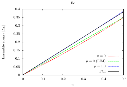
Figure 1: Senjean et al, Phys. Rev. A

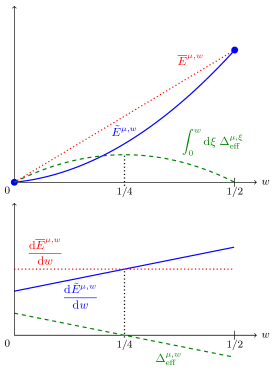
Figure 2: Senjean et al, Phys. Rev. A

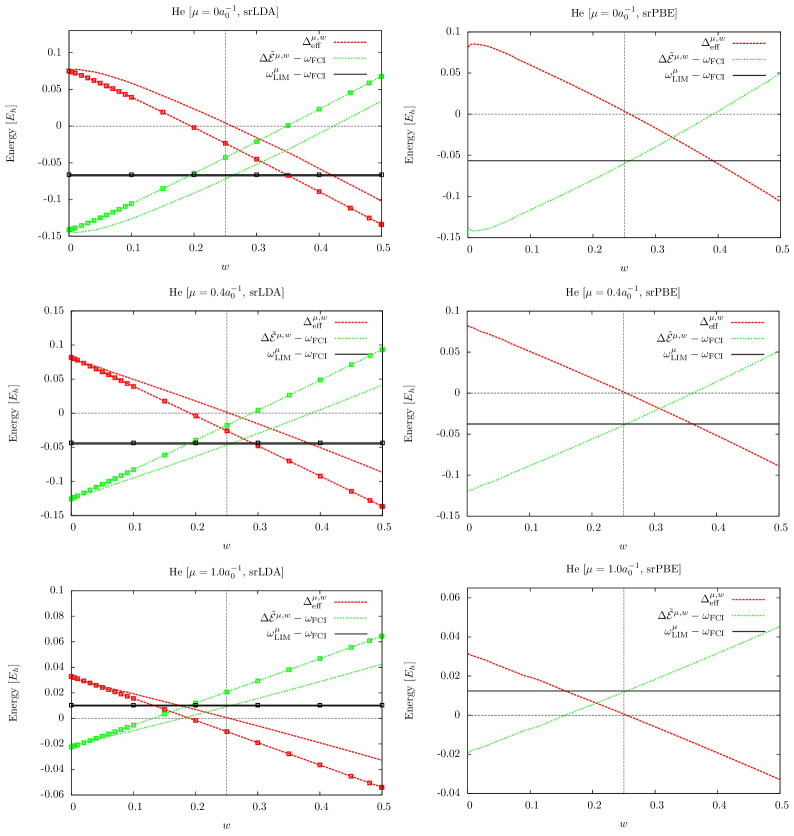
Figure 3: Senjean et al, Phys. Rev. A

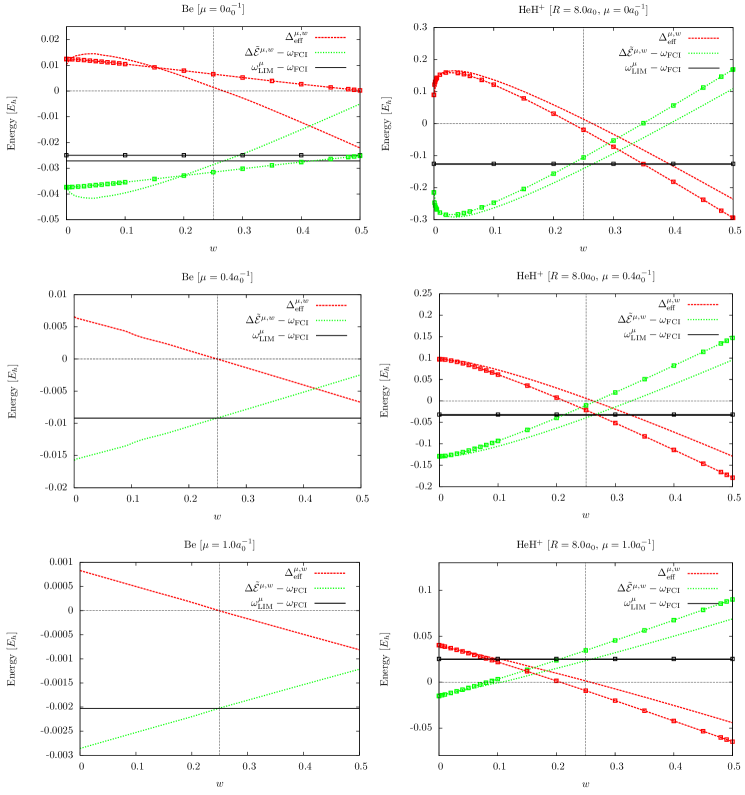
Figure 4: Senjean et al, Phys. Rev. A

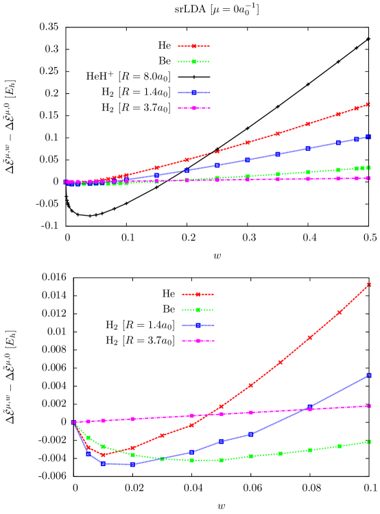
Figure 5: Senjean et al, Phys. Rev. A

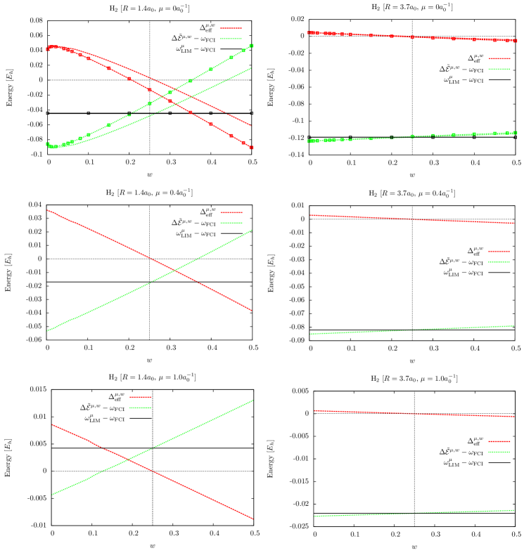
Figure 6: Senjean et al, Phys. Rev. A

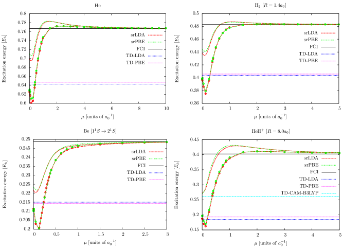
Figure 7: Senjean et al, Phys. Rev. A

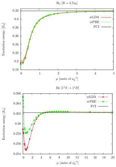
Figure 8: Senjean et al, Phys. Rev. A

References

• Casida and Huix-Rotllant (2012) M. Casida and M. Huix-Rotllant, Annu. Rev. Phys. Chem. 63, 287 (2012).
• Pernal (2012) K. Pernal, J. Chem. Phys. 136, 184105 (2012).
• Rebolini et al. (2013) E. Rebolini, A. Savin,  and J. Toulouse, Mol. Phys. 111, 1219 (2013).
• Fromager et al. (2013) E. Fromager, S. Knecht,  and H. J. Aa. Jensen, J. Chem. Phys. 138, 084101 (2013).
• Hedegård et al. (2013) E. D. Hedegård, F. Heiden, S. Knecht, E. Fromager,  and H. J. A. Jensen, J. Chem. Phys. 139, 184308 (2013).
• Gross et al. (1988a) E. K. U. Gross, L. N. Oliveira,  and W. Kohn, Phys. Rev. A 37, 2805 (1988a).
• Gross et al. (1988b) E. K. U. Gross, L. N. Oliveira,  and W. Kohn, Phys. Rev. A 37, 2809 (1988b).
• Andersson et al. (1992) K. Andersson, P.-Å. Malmqvist,  and B. O. Roos, J. Chem. Phys. 96, 1218 (1992).
• Angeli et al. (2001) C. Angeli, R. Cimiraglia, S. Evangelisti, T. Leininger,  and J. P. Malrieu, J. Chem. Phys. 114, 10252 (2001).
• Angeli et al. (2002) C. Angeli, R. Cimiraglia,  and J.-P. Malrieu, J. Chem. Phys. 117, 9138 (2002).
• Nikiforov et al. (2014) A. Nikiforov, J. A. Gamez, W. Thiel, M. Huix-Rotllant,  and M. Filatov, J. Chem. Phys. 141, 124122 (2014).
• Filatov (2015) M. Filatov, WIREs Comput Mol Sci 5, 146 (2015).
• Pastorczak et al. (2013) E. Pastorczak, N. I. Gidopoulos,  and K. Pernal, Phys. Rev. A 87, 062501 (2013).
• Franck and Fromager (2014) O. Franck and E. Fromager, Mol. Phys. 112, 1684 (2014).
• Yang et al. (2014) Z.-h. Yang, J. R. Trail, A. Pribram-Jones, K. Burke, R. J. Needs,  and C. A. Ullrich, Phys. Rev. A 90, 042501 (2014).
• Pribram-Jones et al. (2014) A. Pribram-Jones, Z.-h. Yang, J. R. Trail, K. Burke, R. J. Needs,  and C. A. Ullrich, J. Chem. Phys. 140, 18A541 (2014).
• Stein et al. (2012) T. Stein, J. Autschbach, N. Govind, L. Kronik,  and R. Baer, J. Phys. Chem. Lett. 3, 3740 (2012).
• Hohenberg and Kohn (1964) P. Hohenberg and W. Kohn, Phys. Rev. 136, B864 (1964).
• Lieb (1983) E. H. Lieb, Int. J. Quantum Chem. 24, 243 (1983).
• Savin (1996) A. Savin, “Recent developments and applications of modern density functional theory,”  (Elsevier, Amsterdam, 1996) p. 327.
• Toulouse et al. (2004a) J. Toulouse, A. Savin,  and H. J. Flad, Int. J. Quantum Chem. 100, 1047 (2004a).
• Toulouse et al. (2004b) J. Toulouse, F. Colonna,  and A. Savin, Phys. Rev. A 70, 062505 (2004b).
• Goll et al. (2005) E. Goll, H. J. Werner,  and H. Stoll, Phys. Chem. Chem. Phys. 7, 3917 (2005).
• Goll et al. (2009) E. Goll, M. Ernst, F. Moegle-Hofacker,  and H. Stoll, J. Chem. Phys. 130, 234112 (2009).
• Ángyán et al. (2005) J. G. Ángyán, I. C. Gerber, A. Savin,  and J. Toulouse, Phys. Rev. A 72, 012510 (2005).
• Fromager et al. (2007) E. Fromager, J. Toulouse,  and H. J. Aa. Jensen, J. Chem. Phys. 126, 074111 (2007).
• Fromager and Jensen (2008) E. Fromager and H. J. Aa. Jensen, Phys. Rev. A 78, 022504 (2008).
• Ángyán (2008) J. G. Ángyán, Phys. Rev. A 78, 022510 (2008).
• Toulouse et al. (2009) J. Toulouse, I. C. Gerber, G. Jansen, A. Savin,  and J. G. Ángyán, Phys. Rev. Lett. 102, 096404 (2009).
• Janesko et al. (2009) B. G. Janesko, T. M. Henderson,  and G. E. Scuseria, J. Chem. Phys. 130, 081105 (2009).
• Leininger et al. (1997) T. Leininger, H. Stoll, H. J. Werner,  and A. Savin, Chem. Phys. Lett. 275, 151 (1997).
• Pollet et al. (2002) R. Pollet, A. Savin, T. Leininger,  and H. Stoll, J. Chem. Phys. 116, 1250 (2002).
• Fromager et al. (2010) E. Fromager, R. Cimiraglia,  and H. J. Aa. Jensen, Phys. Rev. A 81, 024502 (2010).
• Rohr et al. (2010) D. R. Rohr, J. Toulouse,  and K. Pernal, Phys. Rev. A 82, 052502 (2010).
• Hedegård et al. (2015) E. D. Hedegård, S. Knecht, J. S. Kielberg, H. J. Aa. Jensen,  and M. Reiher, J. Chem. Phys. 142, 224108 (2015).
• Savin (2014) A. Savin, J. Chem. Phys. 140, 18A509 (2014).
• Rebolini et al. (2014) E. Rebolini, J. Toulouse, A. M. Teale, T. Helgaker,  and A. Savin, J. Chem. Phys. 141, 044123 (2014).
• Rebolini et al. (2015a) E. Rebolini, J. Toulouse, A. M. Teale, T. Helgaker,  and A. Savin, Phys. Rev. A 91, 032519 (2015a).
• Rebolini et al. (2015b) E. Rebolini, J. Toulouse, A. M. Teale, T. Helgaker,  and A. Savin, Mol. Phys.  (2015b), 10.1080/00268976.2015.1011248.
• Theophilou (1979) A. K. Theophilou, J. Phys. C (Solid State Phys.) 12, 5419 (1979).
• Gidopoulos et al. (2002) N. I. Gidopoulos, P. G. Papaconstantinou,  and E. K. U. Gross, Phys. Rev. Lett. 88, 033003 (2002).
• Pastorczak and Pernal (2014) E. Pastorczak and K. Pernal, J. Chem. Phys. 140, 18A514 (2014).
• Levy (1995) M. Levy, Phys. Rev. A 52, R4313 (1995).
• Kraisler and Kronik (2013) E. Kraisler and L. Kronik, Phys. Rev. Lett. 110, 126403 (2013).
• Kraisler and Kronik (2014) E. Kraisler and L. Kronik, J. Chem. Phys. 140, 18A540 (2014).
• Gould and Toulouse (2014) T. Gould and J. Toulouse, Phys. Rev. A 90, 050502 (2014).
• Aidas et al. (2015) K. Aidas, C. Angeli, K. L. Bak, V. Bakken, R. Bast, L. Boman, O. Christiansen, R. Cimiraglia, S. Coriani, P. Dahle, E. K. Dalskov, U. Ekström, T. Enevoldsen, J. J. Eriksen, P. Ettenhuber, B. Fernández, L. Ferrighi, H. Fliegl, L. Frediani, K. Hald, A. Halkier, C. Hättig, H. Heiberg, T. Helgaker, A. C. Hennum, H. Hettema, E. Hjertenæs, S. Høst, I.-M. Høyvik, M. F. Iozzi, B. Jansík, H. J. Aa. Jensen, D. Jonsson, P. Jørgensen, J. Kauczor, S. Kirpekar, T. Kjærgaard, W. Klopper, S. Knecht, R. Kobayashi, H. Koch, J. Kongsted, A. Krapp, K. Kristensen, A. Ligabue, O. B. Lutnæs, J. I. Melo, K. V. Mikkelsen, R. H. Myhre, C. Neiss, C. B. Nielsen, P. Norman, J. Olsen, J. M. H. Olsen, A. Osted, M. J. Packer, F. Pawlowski, T. B. Pedersen, P. F. Provasi, S. Reine, Z. Rinkevicius, T. A. Ruden, K. Ruud, V. V. Rybkin, P. Sałek, C. C. M. Samson, A. S. de Merás, T. Saue, S. P. A. Sauer, B. Schimmelpfennig, K. Sneskov, A. H. Steindal, K. O. Sylvester-Hvid, P. R. Taylor, A. M. Teale, E. I. Tellgren, D. P. Tew, A. J. Thorvaldsen, L. Thøgersen, O. Vahtras, M. A. Watson, D. J. D. Wilson, M. Ziolkowski,  and H. Ågren, WIREs Comput. Mol. Sci. 4, 269 (2015).
• (48) “Dalton, a molecular electronic structure program, Release Dalton2015 (2015), see http://daltonprogram.org.” .
• Dunning (1989) T. H. Dunning, J. Chem. Phys. 90, 1007 (1989).
• Woon and Dunning (1994) D. E. Woon and T. H. Dunning, J. Chem. Phys. 100, 2975 (1994).
• Vosko et al. (1980) S. H. Vosko, L. Wilk,  and M. Nusair, Can. J. Phys. 58, 1200 (1980).
• Perdew et al. (1996) J. P. Perdew, K. Burke,  and M. Ernzerhof, Phys. Rev. Lett. 77, 3865 (1996).
• Yanai et al. (2004) T. Yanai, D. P. Tew,  and N. C. Handy, Chem. Phys. Lett. 393, 51 (2004).
• Gori-Giorgi and Savin (2009) P. Gori-Giorgi and A. Savin, Int. J. Quantum Chem. 109, 1950 (2009).
• Fromager (2015) E. Fromager, Mol. Phys. 113, 419 (2015).
• Franck et al. (2015) O. Franck, B. Mussard, E. Luppi,  and J. Toulouse, J. Chem. Phys. 142, 074107 (2015).