How are Forbush decreases related to interplanetary magnetic field enhancements ?

Abstract

Aims. A Forbush decrease (FD) is a transient decrease followed by a gradual recovery in the observed galactic cosmic ray intensity. We seek to understand the relationship between the FDs and near-Earth interplanetary magnetic field (IMF) enhancements associated with solar coronal mass ejections (CMEs).

Methods. We used muon data at cutoff rigidities ranging from 14 to 24 GV from the GRAPES-3 tracking muon telescope to identify FD events. We selected those FD events that have a reasonably clean profile, and magnitude $>$ 0.25%. We used IMF data from ACE/WIND spacecrafts. We looked for correlations between the FD profile and that of the one-hour averaged IMF. We wanted to find out whether if the diffusion of high-energy protons into the large scale magnetic field is the cause of the lag observed between the FD and the IMF.

Results. The enhancement of the IMF associated with FDs occurs mainly in the shock-sheath region, and the turbulence level in the magnetic field is also enhanced in this region. The observed FD profiles look remarkably similar to the IMF enhancement profiles. The FDs typically lag behind the IMF enhancement by a few hours. The lag corresponds to the time taken by high-energy protons to diffuse into the magnetic field enhancement via cross-field diffusion.

Conclusions. Our findings show that high-rigidity FDs associated with CMEs are caused primarily by the cumulative diffusion of protons across the magnetic field enhancement in the turbulent sheath region between the shock and the CME.

1 Introduction

Forbush decreases (FDs), are short-term decreases in the intensity of galactic cosmic rays that were first observed by Forbush (1937, 1938). It was the work of Simpson using neutron monitors (Simpson, 1954) that showed that the origin of the FDs was in the interplanetary (IP) medium. Solar transients such as the coronal mass ejections (CMEs) cause enhancements in the interplanetary magnetic field (IMF). The near-Earth manifestation of a CME from the Sun typically has two major components: i) the interplanetary counterpart of CME (commonly called an ICME), and ii) the shock, which is driven ahead of it. Both the shock and the ICME cause significant enhancement in the IMF. Interplanetary CMEs, which possess some well defined criteria such as reduction in plasma temperature and smooth rotation of magnetic field are called magnetic clouds (e.g., Burlaga et al. 1981; Bothmer & Schwenn 1998).

Correlations between the parameters characterizing FDs and solar wind parameters have been a subject of considerable study. Belov et al. (2001) and Kane (2010) maintain that there is a reasonable correlation between the FD magnitude and the product of maximum magnetic field and maximum solar wind velocity. Dumbović et al. (2012) also found reasonable correlation between the FD magnitude $|\rm FD|$, and duration with the solar wind parameters such as the amplitude of magnetic field enhancement B, amplitude of the magnetic field fluctuations $\rm\delta B$, maximum solar wind speed associated with the disturbance v, and duration of the disturbance $\rm t_{B}$. We note that the FD magnitude also depends strongly on other solar wind parameters like the velocity of the CME, turbulence level in the magnetic field, size of the CME, etc. The contributions of these parameters are explained in the CME-only cumulative diffusion model described in Arunbabu et al. (2013).

Arunbabu et al. (2013) described the CME-only cumulative diffusion model for FDs, where the cumulative effects of diffusion of cosmic ray protons through the turbulent sheath region as the CME propagated from the Sun to the Earth was invoked to explain the FD magnitude. However, the diffusion was envisaged to occur across an idealized thin boundary. In this paper we relax the ideal, thin boundary assumption and examine the detailed relationship between the FD profile and the IMF compression.

2 Data analysis

2.1 The GRAPES-3 experiment

The GRAPES-3 experiment is located at Ooty ($11.4^{\circ}$N latitude, $76.7^{\circ}$E longitude, and 2200 m altitude) in India. It contains two major components, first an air shower array of 400 scintillation detectors (each 1 m²), with a distance of 8 m between adjacent detectors deployed in a hexagonal geometry (Gupta et al. 2005, Mohanty et al. 2009, Mohanty et al. 2012). The GRAPES-3 array is designed to measure the energy spectrum and composition of the primary cosmic rays in the energy region from 10 TeV to 100 PeV (Gupta et al. 2009, Tanaka et al. 2012). The second component of the GRAPES-3 experiment, a large area tracking muon telescope is a unique instrument used to search for high-energy protons emitted during the active phase of a solar flare or a CME. The muon telescope provides a high statistics, directional measurement of the muon flux. The GRAPES-3 muon telescope covers an area of 560 m², consisting of a total of 16 modules, each 35 m² in area. The energy threshold of the telescope is sec ($\theta$) GeV for the muons arriving along a direction with zenith angle $\theta$. The observed muon rate of $\sim 3000$ s^-1 per module yields a total muon rate of $\sim 3\times 10^{6}$ min^-1 for the entire telescope (Hayashi et al. 2005, Nonaka et al. 2006). This high rate permits even a small change of $\lesssim 0.1\%$ in the muon flux to be accurately measured over a time scale of $\sim 5$ min, after appropriate corrections are applied for the time dependent variation in the atmospheric pressure (Mohanty et al. 2013).

We identified the FDs using the data from the GRAPES-3 muon telescope. By using the tracking capability of the muon telescope the direction of detected muons are binned into nine different solid angle directions, named NW (northwest), N (north), NE (northeast), W (west), V (vertical), E (east), SW (southwest), S (south), and SE (southeast). The cutoff rigidity due to the geomagnetic field at Ooty is 17 GV along the vertical direction and varies from 14 to 42 GV across the 2.2 sr. field of view of the muon telescope. Details of the muon telescope are given in Hayashi et al. (2005), Nonaka et al. (2006), and Subramanian et al. (2009).

2.2 Broad shortlisting criteria

The GRAPES-3 muon telescope has observed a large number of FD events exhibiting a variety of characteristics. We now describe the broad criteria that we use to shortlist events used for analysis in this paper. In addition to the criteria described here, we will have occasion to apply further criteria, which will be described in subsequent sections. We have examined all FD events observed by the GRAPES-3 muon telescope during the years 2001 – 2004. We shortlist events that have a clean FD profile and FD magnitude $>$ 0.25%, and are also associated with an enhancement in the near-Earth interplanetary magnetic field. Here, the term “clean profile” is used to refer to an FD event characterized by a sudden decrease and a gradual recovery in the cosmic ray flux. Although 0.25 % might seem like a small number, according to Arunbabu et al. (2013) these are fairly significant events in the GRAPES-3 data, given its high sensitivity. This yields a sample of 65 events, which is used in the analysis reported in § 3. We note that the event of 29 September 2001 is not included in this list since it was associated with many IMF enhancements, which could be due to multiple Halo and partial halo CMEs. Similarly, the event of 29 October 2003 is not included (even though it was the biggest FD event observed in the solar cycle 23) since the near-Earth magnetic field data is incomplete for this event.

We used GRAPES-3 data summed over a time interval of one hour for each direction. This improves the signal-to-noise ratio, but the diurnal variation in the muon flux is still present. We used a low-pass filter to remove oscillations having frequency $>$ 1 d^-1. This filter was explained in Subramanian et al. (2009). The measured variation of the muon flux in percent for the 24 November 2001 event is shown in Figure 1, where the dotted black lines are the unfiltered data and the solid black lines are the filtered data after using the low-pass filter to remove the frequencies $>$ 1 d^-1. Although the filtering may change the amplitude of the decrease and possibly shift the onset time for the FD by a few hours in some cases, it is often difficult to determine whether these differences are artifacts of filtering or if the unfiltered data showed different amplitude because a diurnal oscillation happened to have the right phase so as to enhance or suppress the amplitude of the FD. Some fluctuations in the muon flux could be due to FD and associated events, but it is unlikely that they will be periodic in nature and are not likely to be affected by the filter.

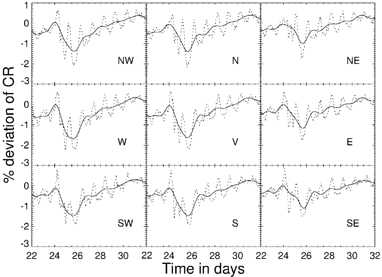
Figure 1: FD event on 24 Nov 2001. Percent deviation in the muon flux for different directions are shown in separate panels. The solid line shows percent deviation for filtered data and the dotted line shows the same for unfiltered data.

The FDs that we study are associated with near-Earth CME counterparts, which contribute to significant increases in the IMFs. We intend to investigate the relation between these IMF enhancements and FDs. We used the IMF data observed by the ACE and WIND spacecraft available from the OMNI database. We used hourly resolution data on magnetic field $\rm B_{total}$, $\rm B_{x}$, $\rm B_{y}$, $\rm B_{z}$ in the geocentric solar ecliptic (GSE) coordinate system: $\rm B_{total}$ is the magnitude of the magnetic field, $\rm B_{x}$ is the magnetic field component along the Sun-Earth line in the ecliptic plane pointing towards the Sun, $\rm B_{z}$ the component parallel to the ecliptic north pole, and $\rm B_{y}$ the component in the ecliptic plane pointing towards dusk. For a consistent data analysis we applied the same low-pass filter to the magnetic field data as we did to the muon flux, which removes any oscillations having frequency $>$ 1 d^-1. Since FD events are associated with enhancements in the IMF, we use the quantity $\rm 100-|B|$ and calculate the average value and the percent deviation of this quantity over the same data interval as the FD. This effectively flips the magnetic field increase and makes it appear as a decrease, enabling easy comparison with the FD profile. Figure 2 shows the FD event on 24 November 2001, 8 shows the FD event on 11 April 2001, and 9 shows the FD event on 23 May 2002, together with the IMF data processed in this manner.

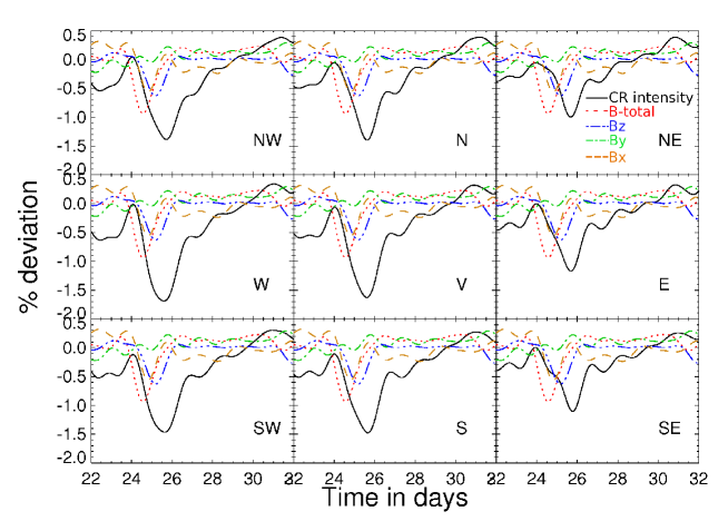
Figure 2: The FD event of 24 Nov 2001 and the magnetic field for 9 directions in GRAPES-3 muon telescope. Black solid line is percentage deviation of cosmic ray intensity in each direction. The red-dotted, blue-dash-dot-dotted, green-dash-dotted and orange-dash lines are percentage deviation of IMFs $\rm B_{total}$, $\rm B_{z}$, $\rm B_{y}$ and $\rm B_{x}$ respectively, that are scaled down by a factor of 10 to fit in the frame.

3 Correlation of FD magnitude with peak IMF

Before studying the detailed relationship between the IMF and FD profiles, we examine the relationship between the peak IMF and the FD magnitudes. For this study we considered all 65 FD events shortlisted using the criteria explained in section 2.2. The FD magnitude for a given direction is calculated as the difference between the pre-event intensity of the cosmic rays and the intensity at the minimum of the decrease. We examine the corresponding IMF during these events. We denote $\rm B_{y}$ and $\rm B_{z}$ “perpendicular” fields, because they are tangential to a flux rope CME approaching the Earth. They are perpendicular to a typical cosmic ray proton that seeks to enter the CME radially; it will therefore have to cross these perpendicular fields. We study the relation between the FD magnitude and the peak of the total magnetic field $\rm B_{total}=\,(B_{x}^{2}+B_{y}^{2}+B_{z}^{2})^{1/2}$ and the peak of the net perpendicular magnetic field $\rm B_{p}\,=\,(B_{y}^{2}+B_{z}^{2})^{1/2}$.

The correlation coefficients of the peak $\rm B_{total}$ with the FD magnitude for different directions are listed in Table 1 and shown in Figure 3. The correlation coefficients of the peak $\rm B_{p}$ with FD magnitude are listed in Table 1 and shown in Figure 4. We find that the correlation coefficient between peak $\rm B_{p}$ and peak $\rm B_{total}$ with the FD magnitude ranges from 63% to 72%. We note that the correlations in Figures 3 and 4 are fairly similar because the longitudinal magnetic field ($B_{x}$) is fairly small for most events. We will have further occasion to discuss this in § 5.1. We also carried out the same study using Tibet neutron monitor data; this yields a correlation coefficient of 60.0% and 61.9% respectively for $\rm B_{total}$ and $\rm B_{p}$. The error on the correlation coefficients are calculated using Eq 1 below, and are listed in Table 1:

$$err=\sqrt{\frac{1-(cc)^{2}}{n-2}}\,.$$ (1)

Here cc is the correlation coefficient, n-2 gives the degree of freedom, and n is the number of points considered for the correlation.

From the CME-only cumulative diffusion model described in Arunbabu et al. (2013) we know that the FD magnitude depends on various parameters associated with CME, such as velocity of CME, turbulence level in the magnetic field, and the size of the CME. It is thus not surprising that the FD magnitude correlates only moderately with the peak value of the IMF.

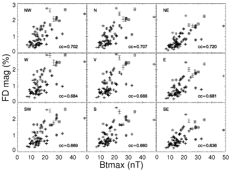
Figure 3: Correlation of maximum total magnetic field in the magnetic field enhancement to FD magnitude observed in different directions using GRAPES-3.

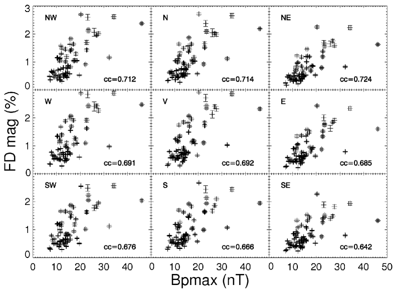
Figure 4: Correlation of maximum perpendicular magnetic field in the magnetic field enhancement to FD magnitude observed in different directions using GRAPES-3.

Table 1: Correlation of the FD magnitude with the maximum total and perpendicular IMF. For each direction of GRAPES-3, the correlation is calculated along with the standard error (err) in the next column. The last row shows the correlation coefficient calculated using data from the Tibet neutron monitor.

Direction	Cut-off	$\rm B_{total}$		$\rm B_{p}$
	Rigidity	Correlation		Correlation
	(GV)	coeff.	err	coeff.	err
NW	15.5	0.702	0.090	0.712	0.089
N	18.7	0.707	0.090	0.714	0.089
NE	24.0	0.720	0.088	0.724	0.088
W	14.3	0.684	0.093	0.691	0.092
V	17.2	0.688	0.092	0.692	0.092
E	22.4	0.681	0.093	0.685	0.093
SW	14.4	0.669	0.094	0.676	0.094
S	17.6	0.660	0.095	0.666	0.095
SE	22.4	0.636	0.098	0.642	0.097
Tibet	14.1	0.600	0.102	0.619	0.100

4 IMF compression: shock-sheath or ICME?

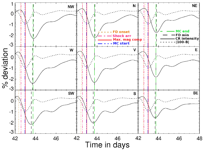
Figure 10: FD event on 11 April 2001. The linestyles are the same as used in figure 5

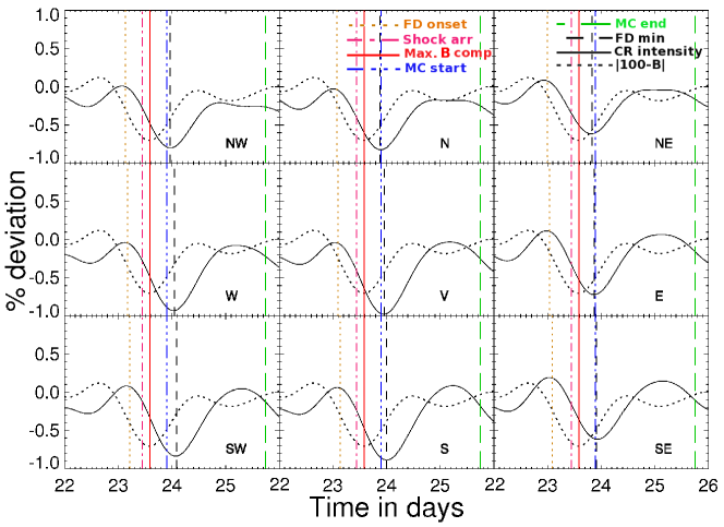
Figure 11: FD event on 23 May 2002. The linestyles are the same as used in figure 5

As mentioned earlier, we considered FD events associated with the magnetic field enhancements that are due to the shock propagating ahead of the ICME. An example of this is shown in Figures 5, 10, and 11 where the nine different panels show the cosmic ray flux (FD profile) of the nine directions of the GRAPES-3 muon telescope for the FD observed on 24 November 2001. It is clear that the magnetic field compression responsible for the FD is in the sheath region, i.e., the region between the shock and magnetic cloud.

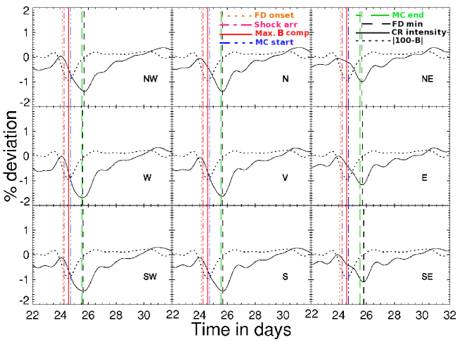
Figure 5: FD event on 24 November 2001. The black solid line denotes percentage deviation of the cosmic ray intensity, black dotted line percentage deviation of total magnetic field $\rm|100-B|$ as explained in §2 which is scaled down to fit the frame. The vertical brown-dotted, magenta-dash-dotted, blue-dash-dot-dotted, green-long-dashed, and black-dashed lines denote the timings corresponding to the FD onset, shock arrival, magnetic cloud start, magnetic cloud end, and FD minimum, respectively. The solid red vertical line corresponds to the maximum of the magnetic field compression.

The CME-only model described in Arunbabu et al. (2013) deals with the diffusion of cosmic rays through the turbulent magnetic field in the sheath region. The cross-field diffusion coefficient depends on the rigidity of the proton and the turbulence level in the magnetic field (e.g., Candia & Roulet 2004). The turbulence level in the magnetic field is an important parameter in this context. We have calculated the turbulence level using one-minute averaged data from the ACE/WIND spacecraft available from the OMNI data base. To calculate the turbulence level $\sigma$ we use a one-hour running average of the magnetic field ($\rm B_{0}$) and the fluctuation of the IMF around this average ($\rm B_{tur}=B-B_{0}$). We define the quantity $\sigma$ as

$$\rm\sigma\,=\,\left(\frac{\langle B_{tur}^{2}\rangle}{B_{0}^{2}}\right)^{0.5},$$ (2)

where $\rm\langle B_{tur}^{2}\rangle$ denotes the average of $\rm B_{tur}^{2}$ over the one-hour window. Figure 6 shows a representative event. The top panel shows the one-minute average magnetic field for 21–30 November 2001. The bottom panel in this figure shows the turbulence level $\sigma$ calculated for this event. We note that the magnetic field compression responsible for the FD occurs in the shock sheath region, i.e., the region between the shock and the magnetic cloud. The turbulence level enhancement also occurs in this region.

For events selected using the criteria described in § 2, we narrow down the ones that have a well-defined shock and associated magnetic cloud. Such events allow us to clearly distinguish the shock, sheath, and CME regions associated with the magnetic field compression. We studied ten such FD events, which are listed in Table 2. The timings of the shock, maximum of the magnetic field compression, magnetic cloud start and end timings, along with the FD onset times for different directions are given in Table 2. The peak of the magnetic field enhancement in the filtered data generally occurs before the start of the magnetic cloud or at the start of the magnetic cloud, whereas in the unfiltered data the enhancement lies in the sheath region. We note that the filtering procedure using the low-pass filter shifts the maximum by a small amount (-5 to 10 hours).

Table 2: Shock arrival time, time of maximum magnetic field enhancement, magnetic cloud start and end timings and FD onset timings for different directions for FD events that have a well-defined shock and magnetic clouds associated with them.

Event	FD onset									Shock	Maximum of	MC	MC
	NW	N	NE	W	V	E	SW	S	SE	arrival	Mag. compre.	Start	end
2001 Apr 04	04.30	04.33	04.29	04.3	04.34	04.32	04.37	04.34	04.25	04.61	04.79	04.87	05.35
2001 Apr 11	11.54	11.58	11.67	11.47	11.50	11.54	11.35	11.43	11.52	11.58	12.00	11.958	12.75
2001 Aug 17	17.18	17.08	17.05	16.97	16.94	16.92	17.00	16.98	16.97	17.45	17.87	18.00	18.896
2001 Nov 24	24.13	24.14	24.13	24.17	24.14	24.12	24.17	24.13	24.06	24.25	24.58	24.708	25.541
2002 May 23	23.13	23.08	23.00	23.17	23.09	23.04	23.21	23.13	23.09	23.44	23.58	23.896	25.75
2002 Sep 07	07.71	07.72	07.67	07.62	07.62	07.63	07.66	07.68	07.71	07.6	08.00	07.708	08.6875
2002 Sep 30	30.56	30.45	30.43	30.56	30.48	30.42	30.52	30.45	30.36	30.31	31.16	30.917	31.6875
2003 Nov 20	19.89	21.34	21.12	20.08	20.45	20.86	20.29	20.43	20.63	20.31	20.67	21.26	22.29
2004 Jan 21	22.09	22.03	21.96	21.98	22.00	21.97	21.83	21.91	21.90	22.09	22.50	22.58	23.58
2004 Jul 26	26.60	26.64	26.75	26.59	26.65	26.75	26.67	26.77	26.86	26.93	27.29	27.08	28.00

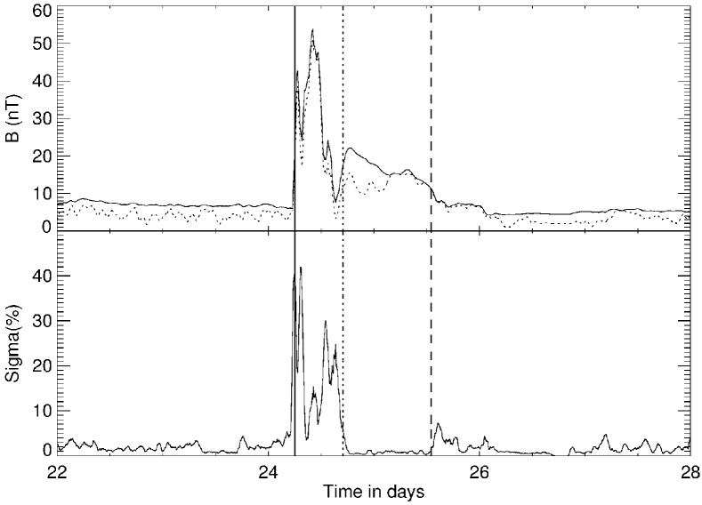
Figure 6: Magnetic field compression associated with the FD event on 24 November 2001. In the first panel the continuous line denotes $\rm B_{total}$ and the dotted line denotes $\rm B_{p}$. The continuous line in the second panel shows the turbulence level for $\rm B_{total}$. In both panels the vertical solid, dotted, and dashed lines corresponds to shock arrival time, magnetic cloud start time, magnetic cloud end time, respectively.

It is clear from Figures 5,   10,   11,  6, and Table 2 that the peak of the magnetic field compression responsible for the FD lies in the sheath region, and the turbulence level is also enhanced in this region. This is in broad agreement with Richardson & Cane (2011).

5 How similar are the FD and the IMF profiles?

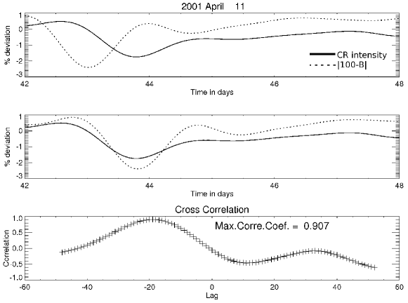
Figure 12: Cross correlation of the cosmic ray flux with $\rm B_{total}$. The top panel shows the percentage deviation of cosmic ray flux using solid black lines and the magnetic field using dotted black lines (scaled to fit in the frame). The middle panel shows the same with magnetic field shifted to the right corresponding to the time lag and the bottom panel shows the correlation coefficient for different lags.

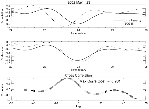
Figure 13: Cross correlation of the cosmic ray flux with $\rm B_{total}$. The top panel shows the percentage deviation of cosmic ray flux using solid black lines and the magnetic field using dotted black lines (scaled to fit in the frame). The middle panel shows the same with magnetic field shifted to the right corresponding to the time lag and the bottom panel shows the correlation coefficient for different lags.

One of the near-Earth effects of a CME is the compression of (and consequent increase in) the IMF. The IMF measured by spacecrafts such as WIND and ACE can detect these magnetic field compressions. We investigate the relation of these magnetic field compressions to the FD profile. We work with the hourly resolution IMF data from the ACE and WIND spacecrafts obtained from the OMNI database. Applying the low-pass filter described in §2 to this data yields a combined magnetic field compression comprising the shock and ICME/magnetic cloud. A visual comparison of the FD profile with the magnetic field compression often reveals remarkable similarities. To quantify the similarity between these two profiles, we studied the cross correlation of the cosmic ray intensity profile with the IMF profile. In order to do this, we shift the magnetic field profile (with respect to the FD profile) by amounts ranging from -36 hours to 12 hours. We identify the peak correlation value and the shift corresponding to this value is considered to be the time lag between the IMF and the cosmic ray FD profile. Most of the FD events exhibit correlations $\geq$ 60% with at least one of the four IMF components ($\rm B_{total}$, $\rm B_{x}$, $\rm B_{y}$, $\rm B_{z}$). Examples of the correlation between the FD profile and $\rm B_{total}$ for the events of 24 November 2001, 11 April 2001, and 23 May 2002 are shown in Figures 7, 12, and 13, respectively. The top panel in these figures shows the percentage deviation of the cosmic ray flux and the $\rm B_{total}$. The percentage deviation of $\rm B_{total}$ is scaled to fit in the frame. The middle panel shows the same percentage deviations, but the magnetic field is shifted by the peak correlation lag and the bottom panel shows the correlation coefficients corresponding to different lags. The correlation lag means that the IMF profile precedes the FD profile by 21 hours for the 24 November 2001 event, by 19 hours for the 11 April 2001 event and 13 hours for the 23 May 2003 event. In particular, Table 3 gives the maximum cross correlation values obtained for different FD profile of different directions of GRAPES-3 to the total magnetic field compression and different components of magnetic field for the 24 November 2001 event. The same quantities for Tibet neutron monitor data are also shown in last row of this table. In further discussion we consider only those events showing a cross correlation $\geq$ 70% for lags between -36 to 12 hours. The events thus shortlisted are presented in Table 5. From these, we will further narrow down events for which the FD profile exhibits a high correlation with the perpendicular component of the IMF.

Table 3: Correlation of FD profile in different direction observed in GRAPES-3 with magnetic fields for the 24 November 2001 event. The numbers in the last row are derived from the Tibet neutron monitor data.

Instrument	dir.	Rg	FD mag.	correlation
		(GV)	(%)	$B_{total}$			$B_{x}$			$B_{y}$			$B_{z}$
				Corr.	err	Lag	Corr.	err	Lag	Corr.	err	Lag	Corr.	err	Lag
				(%)	(%)	(hrs)	(%)	(%)	(hrs)	(%)	(%)	(hrs)	(%)	(%)	(hrs)
	NW	15.5	2.60	80.4	3.8	-23	27.3	6.2	-13	36.3	6.0	-35	73.0	4.4	-13
	N	18.7	2.38	82.3	3.7	-23	29.2	6.2	-16	37.9	6.0	-35	73.8	4.4	-12
GRAPES-3	NE	24.0	1.69	80.7	3.8	-26	26.5	6.2	-19	39.3	5.9	-35	72.6	4.5	-14
	W	14.3	2.85	85.3	3.4	-21	30.1	6.1	-12	40.3	5.9	-30	75.7	4.2	-11
	V	17.2	2.71	85.3	3.4	-21	29.4	6.2	-14	40.5	5.9	-28	76.3	4.2	-11
	E	22.4	2.00	82.1	3.7	-24	29.7	6.2	-17	39.3	5.9	-22	75.5	4.2	-13
	SW	14.4	2.49	84.6	3.4	-21	29.1	6.2	-12	41.0	5.9	-31	74.3	4.3	-11
	S	17.6	2.44	84.9	3.4	-21	31.0	6.1	-14	39.0	6.0	-27	76.6	4.1	-11
	SE	22.4	1.89	81.1	3.8	-26	32.4	6.1	-20	36.8	6.0	-22	77.1	4.1	-14
Tibet		14.1	4.28	87.9	3.1	-20	27.7	6.2	-11	38.9	6.0	-20	75.6	4.2	-8

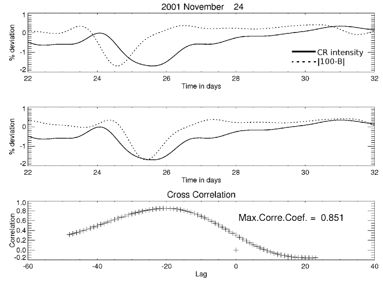
Figure 7: Cross correlation of the cosmic ray flux with $\rm B_{total}$. The top panel shows the percentage deviation of cosmic ray flux using solid black lines and the magnetic field using dotted black lines (scaled to fit in the frame). The middle panel shows the same with magnetic field shifted to the right corresponding to the time lag and the bottom panel shows the correlation coefficient for different lags.

5.1 Cross-field diffusion into the ICME through the sheath

The time lag between the cosmic ray flux and the IMF occurs because the high-energy protons do not respond to magnetic field compressions immediately; they are subjected to the classical magnetic mirror effect arising from the gradient in the longitudinal magnetic field and to turbulent cross-field (also referred as perpendicular) diffusion (e.g., Kubo & Shimazu, 2010). Here, we concentrate only on the cross-field diffusion of the high-energy protons through the turbulent sheath region between the shock and the CME. As discussed earlier, we have identified the IMF compression to be comprised mainly of this sheath region; we therefore use the observed values of the mean field and turbulent fluctuations in the sheath region to calculate representative diffusion timescales for cosmic rays. The time delay between the IMF compression and the FD profile (i.e., the correlation lag) can be interpreted as the time taken by the cosmic rays to diffuse into the magnetic compression. Our approach may be contrasted with that of Kubo & Shimazu, (2010), who use a computational approach to investigate cosmic ray dynamics (thus incorporating both the mirror effect and cross-field diffusion) in a magnetic field configuration that comprises an idealized flux rope CME. They do not consider the sheath region, and neither do they use observations to guide their choice of magnetic field turbulence levels.

To calculate the cross-field diffusion timescale, we proceed as follows: considering the flux rope geometry of a near-Earth CME, the magnetic field along the Sun-Earth ($\rm B_{X}$) represents the longitudinal magnetic field. The fields $\rm B_{y}$ and $\rm B_{z}$ represent the perpendicular magnetic fields encountered by the diffusing protons. In our discussion we consider only cross-field diffusion; we therefore choose events that exhibit good correlation with the $\rm B_{y}$ and $\rm B_{z}$ magnetic field compressions and poor correlation with compressions in $\rm B_{x}$. The events shortlisted using these criteria are listed in Table 4.

Table 4: Events for which the FD profile correlates well only with the perpendicular component of the IMF enhancement. These events are a subset of the events listed in Table 5. The associated CMEs are also listed. The correlation lags are given in hours.

Event	CME	Time	type	$\rm V_{m}$	$\rm B_{total}$		$\rm B_{y}$		$\rm B_{z}$
	(near Sun)	(UT)		$\rm km\,s^{-1}$	Corr.(%)	Lag (hrs)	Corr.(%)	Lag (hrs)	Corr.(%)	Lag (hrs)
2001 Jan 13	Jan 10	00:54	Halo	832	97.2	-13	95.8	-14	96.6	-23
2001 Apr 11	Apr 10	05:30	Halo	2411	90.7	-19	89.9	-17	91.3	-5
2001 May 27	May 25	04:06	354	569	66.5	0	65.0	-3	75.7	-21
2001 Aug 13	Aug 11	04:30	313	548	51.8	-7	97.5	-7	70.0	-5
2001 Sep 12	Sep 11	14:54	Halo	791	79.2	-25	26.7	-30	86.2	-1
2001 Nov 24	Nov 22	23:30	Halo	1437	85.3	-21	41.0	-31	77.1	-14
2001 Dec 14	Dec 13	14:54	Halo	864	74.7	-35	69.7	-2	72.8	-17
2002 Sep 07	Sep 05	16:54	Halo	1748	77.1	-18	49.6	-24	87.4	3
2002 Sep 30	Sep 29	15:08	261	958	81.1	-5	72.1	8	75.7	-12
2002 Dec 22	Dec 19	22:06	Halo	1092	73.4	-15	43.4	0	84.7	-12
2003 Jan 23	Jan 22	05:06	338	875	70.9	-21	-	-	75.4	-28
2003 Feb 16	Feb 14	20:06	256	796	-	-	-	-	74.3	-11
2003 May 04	May 02	12:26	222	595	83.4	-8	84.7	-10	80.7	0
2003 Jul 25	Jul 23	05:30	302	543	95.3	-19	73.3	-2	41.6	2
2003 Dec 27	Dec 25	09:06	257	178	86.1	-35	21.7	5	87.2	-3
2004 Aug 30	Aug 29	02:30	274	1195	-	-	-	-	92.4	1
2004 Dec 05	Dec 03	00:26	Halo	1216	85.3	-12	89.4	8	58.4	-13
2004 Dec 12	Dec 08	20:26	Halo	611	81.1	-17	73.3	-25	78.9	-13

6 Cross-field diffusion coefficient ($\rm D_{\perp}$)

The cross-field diffusion coefficient $\rm D_{\perp}$ governs the diffusion of the ambient high-energy protons into the CME across the magnetic fields that enclose it. The topic of cross-field diffusion of charged particles across magnetic field lines in the presence of turbulence is the subject of considerable research. Analytical treatments include classical scattering theory (e.g., Giacalone & Jokipii 1999, and references therein) and non-linear guiding center theory (Matthaeus et al. 2003; Shalchi, 2010) for cross-field diffusion. Numerical treatments of cross-field diffusion of charged particle in turbulent magnetic fields include Giacalone & Jokipii (1999), Casse, Lemoine, & Pelletier (2002), Candia & Roulet (2004), Tautz & Shalchi (2011), and Potgieter et al. (2014). We seek a concrete prescription for $\rm D_{\perp}$ that can incorporate observationally determined quantities.

6.1 $\rm D_{\perp}$: Candia & Roulet (2004)

The $\rm D_{\perp}$ prescription we use is given by Candia & Roulet (2004), obtained from extensive Monte Carlo simulations of cosmic rays propagating through tangled magnetic fields. Their results reproduce the standard results of Giacalone & Jokipii (1999) and Casse, Lemoine, & Pelletier (2002), and also extend the regime of validity to include strong turbulence and high rigidities. The extent of cross-field diffusion of protons depends on the proton rigidity, which indicates how tightly the proton is bound to the magnetic field, and the level of magnetic field turbulence, which can contribute to field line transport.

Candia & Roulet (2004) give the following fit for the “parallel” diffusion coefficient $\rm D_{\parallel}$ (which is due to scattering of the particles back and forth along the mean field, as the field is subject to random turbulent fluctuations),

$$\textit{D}_{\parallel}\equiv cL_{max}\rho\frac{N_{\parallel}}{\sigma^{2}}\sqrt{\left(\frac{\rho}{{\rho}_{\parallel}}\right)^{2(1-\gamma)}+\left(\frac{\rho}{{\rho}_{\parallel}}\right)^{2}}$$ (3)

where c is the speed of light and the quantities $\rm N_{\parallel}$, $\gamma$, and $\rm{\rho}_{\parallel}$ are constants specific to different kinds of turbulence whose values are listed in Table 1 of Candia & Roulet (2004). The parameter $\rm L_{max}$ is the maximum length scale of turbulence; in our case we considered it as the size of the CME near the Earth. The quantity $\rho$ is related to the rigidity of the proton $\rm Rg$ as

$$\rm\rho\,=\,\frac{r_{L}}{L_{max}}\,=\,\frac{Rg}{B_{0}L_{max}},$$ (4)

where $\rm r_{L}$ is the Larmor radius and $\rm B_{0}$ is the magnetic field. The quantity $\sigma^{2}$ is the magnetic turbulence level, which is defined as in Eq. 2.

The cross-field diffusion coefficient ($\rm D_{\perp}$) is related to the parallel one ($\rm D_{\parallel}$ ) by,

$$\rm\frac{D_{\perp}}{D_{\parallel}}\equiv\cases{N_{\perp}{\left(\sigma^{2}\right)}^{a_{\perp}},&$(\rho\leq 0.2)$\cr\vskip 6.0pt plus 2.0pt minus 2.0pt\cr N_{\perp}{\left(\sigma^{2}\right)}^{a_{\perp}}\left(\frac{\rho}{0.2}\right)^{-2},&$(\rho\geq 0.2)$}$$

The quantities $\rm N_{\perp}$ and $\rm a_{\perp}$ are constants specific to different kinds of turbulent spectra, and are given in Table 1 of Candia & Roulet (2004). We note that the exponent characterizing the IMF turbulence may vary through the magnetic field compression associated with FD (Alania & Wawrzynczak, 2012). Although the treatment of Candia & Roulet (2004), which we use, cannot accommodate arbitrary turbulent spectrum indices, it can address the Kolmogorov ($\gamma$ = 5/3), Kraichnan ($\gamma$ = 3/2), and Bykov–-Toptygin ($\gamma$ = 2) spectra. We therefore quote results for all three turbulence spectra.

7 The IP B field compression-FD lag: how many diffusion lengths?

We have shown that the FD profile is often very similar to that of the IMF compression, and lags behind it by a few hours. This observed lag is poorly correlated with the FD magnitude and the CME speeds (both near the Sun and near the Earth). We interpret the observed time lag between the IMF and the FD profiles as the time taken by the protons to diffuse through the magnetic field compression via cross-field diffusion. The time taken for a single diffusion random walk of a high-energy proton into the magnetic structure of CME is given by

$$t_{diff}=\frac{D_{\perp}}{cV_{sw}},$$ (5)

where c is the speed of light (which is the typical propagation speed for the highly relativistic galactic cosmic rays we are concerned with) and $\rm V_{sw}$ is the solar wind velocity upstream of the CME.

When using the $\rm D_{\perp}$ from Candia & Roulet (2004), we use two different methods for computing the turbulence level $\sigma$. In the first one, we calculate $\sigma$ as a function of time using the one-minute averaged IMF data, as described in Eq (2). In the second, we assume a constant value of 15% for $\sigma$, which is typically expected to be the maximum level of turbulence in quiet solar wind (Spangler, 2002). We used both these methods to calculate $\rm t_{diff}$ for Kolmogorov, Kraichnan, and Bykov-Toptygin turbulent spectra. Using these values of $\rm t_{diff}$, we estimated the number of diffusion lengths required to account for the observed time lag between the FD profile and the IMF profile using

$${\rm No.\,of\,Diffusions\,=\frac{Lag}{t_{diff}}}$$ (6)

The results for the number of diffusion times needed to account for the observed lag between the IMF enhancement and the FD profile are shown in Table 6. These numbers are calculated using the peak value of the IMF profile. It is evident that the observed lags can be accounted for by a few tens to a few hundred diffusion times. There are two exceptional events on 2001 December 14 and 2003 December 27, where the number of diffusions are $\sim$1000 using the time-varying $\sigma$ prescription. There are three events in this list that have no correlation lag between the IMF profile and FD profile. The FD on 2001 May 27 correlates well with $\rm B_{total}$, the FD on 2002 December 22 correlates well with $\rm B_{y}$, and the FD on 2003 May 04 correlates with the $\rm B_{z}$ with no correlation lag.

8 Summary

We studied all FD events observed by the GRAPES-3 muon telescope during the years 2001–2004 satisfying the broad criteria listed in § 2.2. For a sample of especially well-observed events, we find that the magnetic field compression responsible for the FD as well as the turbulence level gets enhanced in the shock-sheath region. For these events, details regarding shock timing, magnetic cloud start and end timings along with the FD onset time for different directions are given in Table 2.

We find that the FD profile looks remarkably similar to that of the corresponding IMF compression and lags behind it by few hours (Table 5). Since we want to focus on cross-field diffusion, we selected the FD events whose profiles correlate well with the enhancements in the perpendicular magnetic fields ($\rm B_{y}$, $\rm B_{z}$) and not with the radial magnetic field ($\rm B_{x}$); these events are listed in Table 4. We have calculated the number of diffusions using Eq 6 for 14.3 GV and 24.0 GV protons. The number of diffusions corresponding to the observed lag for the selected events are listed in Table 6. For most events we find that the observed time lag corresponds to a few tens to a few hundred diffusions.

9 Conclusion

The results of Arunbabu et al. (2013) show that FDs are due to cumulative diffusion of galactic cosmic ray protons into the CME as it propagates from the Sun to the Earth. However, the precise nature of the diffusive barrier was left unspecified, and the diffusion was assumed to occur across an idealized thin boundary that presumably had to do with the turbulent sheath region. The results from this work clearly show that the magnetic field enhancement responsible for the FD comprises the sheath region. The FD profile looks like a lagged (and inverted) copy of the magnetic field enhancement (Table 1). The FD lags behind the magnetic field enhancement by a few hours (Tables 5 and 4). We have quantitatively shown that the time lag between the FD and the magnetic field enhancement can be accounted for by cross-field diffusion through the turbulent sheath region (Table 6). This work establishes i) the importance of the turbulent sheath region between the shock and ICME; we show that the magnetic field enhancement responsible for the FD comprises the shock-sheath, and the magnetic turbulence level is also enhanced in this region (§ 4) and ii) the viability of cross-field diffusion through the turbulent CME sheath as the primary mechanism for FDs (§ 7).

Appendix A Additional figures

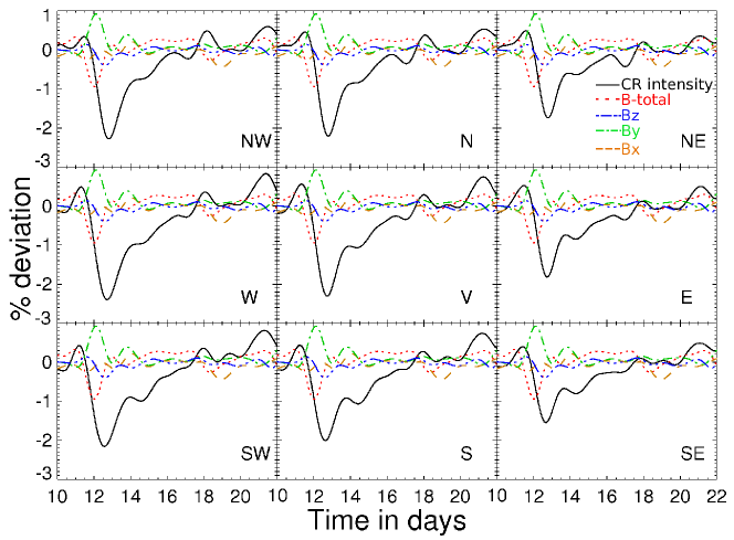
Figure 8: The FD event of 11 April 2001 and the magnetic field for nine directions in GRAPES-3 muon telescope. The linestyles are the same as used in Figure 2

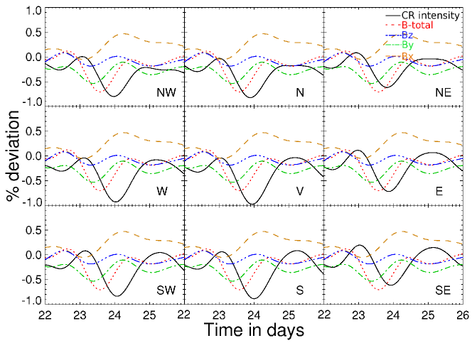
Figure 9: The FD event of 23 May 2002 and the magnetic field for nine directions in GRAPES-3 muon telescope. The linestyles are the same as used in Figure 2

Appendix B Additional Tables

Table 5: List of FD events for which the correlation coefficient between the profiles of the FD and the IMF enhancement $\geq$ 70%. The ‘-’ entries denote events that have low correlation values for lags between -36 and 12 hours

Event	Correlation (%)
	$\rm B_{total}$		$\rm B_{x}$		$\rm B_{y}$		$\rm B_{z}$
	coeff.	err	coeff.	err	coeff.	err	coeff.	err
13 Jan 2001	97.2	2.4	-	-	95.8	2.9	96.6	2.6
26 Mar 2001	70.3	6.5	-	-	-	-	39.1	8.3
4 Apr 2001	92.8	3.1	97.3	1.9	77.2	5.3	63.4	6.4
7 Apr 2001	94.3	3.0	92.7	3.4	71.9	6.2	54.2	7.7
11 Apr 2001	90.7	3.5	-	-	89.9	3.7	91.3	3.4
27 May 2001	66.5	7.7	27.8	9.8	65.0	7.7	75.7	6.7
1 Jun 2001	77.1	4.9	70.5	5.4	52.3	6.6	54.5	6.5
13 Aug 2001	51.8	7.2	-	-	97.5	1.8	70.0	5.9
17 Aug 2001	84.6	3.8	-	-	31.2	6.8	58.0	5.9
6 Sep 2001	68.8	6.1	87.0	4.1	64.7	6.3	45.1	7.5
12 Sep 2001	79.2	4.2	56.2	5.6	26.7	6.6	86.2	3.5
29 Sep 2001	70.3	4.0	-	-	58.1	4.6	-	-
5 Nov 2001	88.3	3.0	64.6	4.9	34.8	6.1	-	-
24 Nov 2001	85.3	3.4	32.4	6.1	41.0	5.9	77.1	4.1
14 Dec 2001	74.7	3.5	42.7	4.8	69.7	3.8	72.8	3.6
23 May 2002	98.1	2.0	79.4	6.2	75.9	6.7	60.0	8.2
7 Sep 2002	77.1	4.6	-	-	49.6	6.3	87.4	3.5
23 Sep 2002	60.4	5.8	87.9	3.5	41.4	6.6	93.1	2.6
30 Sep 2002	81.1	5.3	58.7	7.4	72.1	6.3	75.7	6.0
22 Dec 2002	73.4	4.9	-	-	43.4	6.5	84.7	3.8
9 Jan 2003	90.1	3.3	68.1	6.7	-	-	56.2	6.4
23 Jan 2003	70.9	6.4	-	-	-	-	75.4	6.0
30 Jan 2003	94.8	3.7	84.4	6.4	42.7	10.7	95.7	3.4
16 Feb 2003	-	-	31.3	5.3	-	-	74.3	3.7
26 Mar 2003	77.1	3.8	64.8	4.5	-	-	-	-
4 May 2003	83.4	5.6	32.8	9.7	84.7	5.4	80.7	6.1
18 May 2003	86.5	3.6	-	-	-	-	-	-
25 Jul 2003	95.3	2.8	47.9	8.0	73.3	6.2	41.6	8.3
16 Aug 2003	71.6	6.4	49.6	8.0	45.5	8.2	57.7	7.5
21 Oct 2003	80.1	6.1	92.0	4.0	70.1	7.3	93.5	3.6
27 Dec 2003	86.1	4.2	-	-	21.7	8.1	87.2	4.1
21 Jan 2004	77.9	4.0	78.2	4.0	-	-	-	-
29 May 2004	53.1	6.6	90.2	3.3	-	-	86.9	3.8
26 Jul 2004	86.5	4.2	73.3	5.7	85.5	4.3	94.8	5.6
30 Aug 2004	-	-	-	-	-	-	92.4	2.9
5 Dec 2004	85.3	3.1	-		89.4	2.6	58.4	4.8
12 Dec 2004	81.1	4.2	61.6	5.7	73.3	4.9	78.9	4.4

Table 6: Number of diffusions required for the observed lag in FD events using three different turbulent spectrums and two different methods described in §7. $\rm 1^{st}$ stands for the method using dynamic $\sigma$, $\rm 2^{nd}$ stands for the method using a constant $\sigma$.

	$\sigma$	Rg	$\rm B_{total}$							$\rm B_{y}$							$\rm B_{z}$
Event			Lag	No: of diffusions						Lag	No: of diffusions						Lag	No: of diffusions
	(%)	(GV)	(hrs)	Kolmo.		Kraich.		Bykov.		(hrs)	Kolmo.		Kraich.		Bykov.		(hrs)	Kolmo.		Kraich.		Bykov.
				$\rm 1^{st}$	$\rm 2^{nd}$	$\rm 1^{st}$	$\rm 2^{nd}$	$\rm 1^{st}$	$\rm 2^{nd}$		$\rm 1^{st}$	$\rm 2^{nd}$	$\rm 1^{st}$	$\rm 2^{nd}$	$\rm 1^{st}$	$\rm 2^{nd}$		$\rm 1^{st}$	$\rm 2^{nd}$	$\rm 1^{st}$	$\rm 2^{nd}$	$\rm 1^{st}$	$\rm 2^{nd}$
2001 Jan 13	8-15	14.3	-13	384	173	462	210	644	265	-14	196	158	232	186	314	251	-23	97	112	115	133	133	155
		24.0	-13	245	121	292	140	395	188	-14	117	95	137	110	172	137	-23	38	44	47	55	49	57
2001 Apr 11	10-23	14.3	-19	656	340	895	482	907	396	-17	326	292	425	394	453	372	-5	41	67	47	81	64	102
		24.0	-19	533	283	670	367	844	390	-17	258	239	312	296	409	356	-5	25	47	28	54	37	73
2001 May 27	8-13	14.3	0	0	0	0	0	0	0	-3	44	38	53	46	71	59	-21	111	177	128	205	165	270
		24.0	0	0	0	0	0	0	0	-3	29	25	34	29	45	38	-21	53	85	63	101	70	114
2001 Aug 13	10-20	14.3	-7	216	106	279	135	326	150	-7	76	86	91	102	120	135	-5	26	58	30	69	40	92
		24.0	-7	165	82	199	97	273	130	-7	49	55	57	64	73	83	-5	15	35	17	41	21	52
2001 Sep 12	10-20	14.3	-25	838	354	1046	441	1357	526	-	-	-	-	-	-	-	-1	17	13	20	16	26	20
		24.0	-25	583	263	695	307	953	415	-	-	-	-	-	-	-	-1	11	9	13	11	18	14
2001 Nov 24	20-40	14.3	-21	822	405	1119	578	1137	462	-31	173	429	205	529	241	646	-14	260	226	331	296	381	301
		24.0	-21	666	338	834	442	1067	456	-31	112	311	126	363	165	490	-14	199	181	235	219	319	281
2001 Dec 14	5-12	14.3	-35	1346	604	1644	817	2283	766	-2	56	28	67	35	92	42	-17	255	240	305	298	396	357
		24.0	-35	872	494	1066	614	1440	736	-2	28	21	34	25	41	33	-17	119	177	145	206	165	279
2002 Sep 07	5-20	14.3	-18	776	298	983	396	1255	393	-24	312	305	367	368	499	476	3	24	37	28	45	38	59
		24.0	-18	555	241	667	295	928	369	-24	172	205	204	238	245	313	3	14	25	16	29	20	37
2002 Sep 30	10-20	14.3	-5	207	93	294	131	362	210	8	130	128	160	167	198	174	-12	198	185	243	238	309	259
		24.0	-5	171	77	224	99	254	108	8	93	102	109	123	148	159	-12	138	145	162	173	217	229
2002 Dec 22	5-13	14.3	-15	481	244	617	321	779	327	0	0	0	0	0	0	0	-12	66	126	75	147	100	199
		24.0	-15	363	196	436	238	603	303	0	0	0	0	0	0	0	-12	37	70	42	82	50	99
2003 Jan 23	8-18	14.3	-21	509	270	624	327	823	420	-	-	-	-	-	-	-	-28	49	170	56	200	66	243
		24.0	-21	341	183	403	213	540	281	-	-	-	-	-	-	-	-28	21	71	24	87	25	93
2003 Feb 16	5-17	14.3	-	-	-	-	-	-	-	-	-	-	-	-	-	-	11	55	100	64	117	76	155
		24.0	-	-	-	-	-	-	-	-	-	-	-	-	-	-	-11	22	50	27	60	29	69
2003 May 04	10-40	14.3	-8	252	127	334	165	374	174	-10	97	125	115	149	150	195	0	0	0	0	0	0	0
		24.0	-8	200	101	245	121	325	157	-10	64	82	73	95	95	124	0	0	0	0	0	0	0
2003 Jul 25	8-15	14.3	-19	565	347	732	483	861	417	-2	32	31	39	40	50	43	2	9	22	10	26	13	35
		24.0	-19	434	288	554	367	704	408	-2	22	24	26	29	34	38	2	5	13	6	15	7	19
2003 Dec 27	4-12	14.3	-35	1210	506	1546	634	1881	742	5	41	52	48	61	64	82	-3	10	27	11	31	16	19
		24.0	-35	900	380	1079	446	1497	603	5	23	29	27	34	32	41	-3	5	13	6	16	6	18
2004 Aug 30	8-20	14.3	-	-	-	-	-	-	-	-	-	-	-	-	-	-	1	10	12	12	15	16	19
		24.0	-	-	-	-	-	-	-	-	-	-	-	-	-	-	1	7	8	8	9	10	12
2004 Dec 05	10-23	14.3	-12	326	209	435	285	530	363	8	107	112	128	140	168	198	-13	117	193	146	244	166	278
		24.0	-12	260	172	327	215	403	254	8	71	83	82	97	107	131	-13	89	148	104	174	138	235
2004 Dec 12	5-20	14.3	-17	595	266	786	344	863	368	-25	243	322	290	389	373	500	-13	138	163	165	196	214	255
		24.0	-17	469	210	573	251	771	330	-25	163	218	187	253	245	335	-13	91	108	106	126	137	164