On the BLM optimal renormalization scale

setting for semihard processes

F. Caporale^1∗, D.Yu. Ivanov^2¶, B. Murdaca^3† and A. Papa^3†

¹ Instituto de Física Teórica, Universidad Autónoma de Madrid,

E-28049 Madrid, Spain

² Sobolev Institute of Mathematics and Novosibirsk State University,

RU-630090 Novosibirsk, Russia

³ Dipartimento di Fisica, Università della Calabria,

and Istituto Nazionale di Fisica Nucleare, Gruppo collegato di Cosenza,

I-87036 Arcavacata di Rende, Cosenza, Italy

The BFKL approach for the investigation of semihard processes is plagued by large next-to-leading corrections, both in the kernel of the universal BFKL Green’s function and in the process-dependent impact factors, as well as by large uncertainties in the renormalization scale setting. All that calls for some optimization procedure of the perturbative series. In this respect, one of the most common methods is the Brodsky-Lepage-Mackenzie (BLM) one, that eliminates the renormalization scale ambiguity by absorbing the non-conformal $\beta_{0}$-terms into the running coupling. In this paper, we apply BLM scale setting procedure directly to the amplitudes (cross sections) of several semihard processes. We show that, due to the presence of $\beta_{0}$-terms in the next-to-leading expressions for the impact factors, the optimal renormalization scale is not universal, but depends both on the energy and on the type of process in question.

$\begin{array}[]{ll}{}^{\ast}\mbox{{\it e-mail address:}}&\mbox{francesco.caporale@uam.es}\\ {}^{\P}\mbox{{\it e-mail address:}}&\mbox{d-ivanov@math.nsc.ru}\\ {}^{\dagger}\mbox{{\it e-mail address:}}&\mbox{beatrice.murdaca, alessandro.papa \ @fis.unical.it}\\ \end{array}$

1 Introduction

We discuss the application of the BFKL method [1] to the description of semihard processes, i.e. hard processes in the kinematic region where the energy variable $s$ is substantially larger than the hard scale $Q^{2}$, $s\gg Q^{2}\gg\Lambda_{\rm QCD}^{2}$, with $Q$ the typical transverse momentum and $\Lambda_{\rm QCD}$ the QCD scale. This approach allows to resum systematically to all orders of perturbation series the terms enhanced by leading $\alpha_{s}^{n}\ln^{n}(s/Q^{2})$ (LLA) and first subleading $\alpha_{s}^{n+1}\ln^{n}(s/Q^{2})$ (NLA) logarithms of the energy.

In the BFKL approach, relevant physical observables are expressed as a convolution of two impact factors with the Green’s function of the BFKL equation. The Green’s function is determined through the BFKL equation and is process-independent. The next-to-leading order (NLO) kernel of the BFKL equation for singlet color representation in the $t$-channel and forward scattering, relevant for the determination of the NLA total cross section, has been achieved in Refs. [2], after the long program of calculation of the NLO corrections [3] (for a review, see Ref. [4]). The other essential ingredient are impact factors, which are not universal and must be calculated process by process. Indeed, only a few of them are known with NLO accuracy.

Both the impact factors and the BFKL kernel receive large NLO corrections in the $\overline{\rm{MS}}$ renormalization scheme. The practical application of this approach to physical processes encounters therefore serious difficulties, due not only to the large NLO corrections, but also to big renormalization scale setting uncertainties, thus calling for some optimization procedure of the QCD perturbative series.

In this paper we focus on the widely-used Brodsky-Lepage-Mackenzie (BLM) approach [5] to face with this problem, which relies on the removal of the renormalization scale ambiguity by absorbing the non-conformal $\beta_{0}$-terms into the running coupling. It is known that after BLM scale setting, the QCD perturbative convergence can be greatly improved due to the elimination of renormalon terms in the perturbative QCD series. Moreover, with the BLM scale setting, the BFKL Pomeron intercept has a weak dependence on the virtuality of the Reggeized gluon [6, 7].

We apply the BLM scale setting procedure directly to the amplitudes (cross sections) of several semihard processes. It is shown that due to the presence of $\beta_{0}$-terms in the NLO expressions for the impact factors, the resulting optimal renormalization scale is not universal and depends both on the energy and on the type of process in question. We illustrate this general conclusion considering in details the following semihard processes:

• the forward amplitude of production of two light vector mesons in collision of two virtual photons, $\gamma^{*}\gamma^{*}\to V_{1}V_{2}$;

• the high-energy behavior of the total cross section for highly virtual photons, $\gamma^{*}\gamma^{*}\to X$;

• the inclusive production of two forward, high-$p_{T}$ jets separated by a large interval in rapidity $\Delta y$ (Mueller-Navelet jets), $p+p\to{\rm jet}+{\rm jet}+X$.

At present we do not have a model-independent method to resum the BFKL series beyond the NLA logarithms of the energy. Therefore we strictly adhere here to the original formulation of the BLM procedure and do not consider its higher-order extensions, such as the sequential extended BLM [8] and the Principle of Maximum Conformality [9] (see [10] for a review on the latter method; see also [11, 13, 12, 14] for some recent comparisons between different optimization methods).

The paper is organized as follows: in section 2 we rederive the general expression for the NLA BFKL amplitude in the $(\nu,n)$-representation; in section 3 we discuss in detail the implementation of the BLM scale setting method, both in exact way and in some approximated forms; in section 4 we present the applications of the procedure to the three different processes mentioned above; finally, in section 5 we draw our conclusions and discuss previous studies of semihard processes with BLM method.

2 The BFKL amplitude

The cross section and many other physical observables are directly related to the forward amplitude, which in the BFKL approach can be expressed as follows:

$${\rm Im}_{s}\left({\cal A}\right)=\frac{s}{(2\pi)^{2}}\int\frac{d^{2}\vec{q}_{1}}{\vec{q}_{1}^{\,\,2}}\Phi_{1}(\vec{q}_{1},s_{0})\int\frac{d^{2}\vec{q}_{2}}{\vec{q}_{2}^{\,\,2}}\Phi_{2}(-\vec{q}_{2},s_{0})\int\limits^{\delta+i\infty}_{\delta-i\infty}\frac{d\omega}{2\pi i}\left(\frac{s}{s_{0}}\right)^{\omega}G_{\omega}(\vec{q}_{1},\vec{q}_{2})\,.$$ (1)

This expression holds with NLA accuracy. Here, $s$ is the squared center-of-mass energy, whereas $s_{0}$ is an artificial scale introduced to perform the Mellin transform from the $s$-space to the complex angular momentum plane and cancels in the full expression, up to terms beyond the NLA. All momenta entering this expression are defined on the transverse plane and are therefore two-dimensional. $\Phi_{1,2}$ are the NLO impact factors specific of the process; we will see later on three different examples for them. The Green’s function $G_{\omega}$ takes care of the universal, energy-dependent part of the amplitude. It obeys the BFKL equation

$$\omega\,G_{\omega}(\vec{q}_{1},\vec{q}_{2})=\delta^{(2)}(\vec{q}_{1}-\vec{q}_{2})+\int d^{2}\vec{q}\,K(\vec{q}_{1},\vec{q})\,G_{\omega}(\vec{q},\vec{q}_{1})\;,$$ (2)

where $K(\vec{q}_{1},\vec{q}_{2})$ is the BFKL kernel.

In this section we will derive a general form for the amplitude in the so-called $(\nu,n)$-representation, which will provide us with the starting point of our further analysis. We will proceed along the same lines of Refs. [15]. First of all, it is convenient to work in the transverse momentum representation, defined by

$$\hat{\vec{q}}\>|\vec{q}_{i}\rangle=\vec{q}_{i}|\vec{q}_{i}\rangle\;,$$ (3)

$$\langle\vec{q}_{1}|\vec{q}_{2}\rangle=\delta^{(2)}(\vec{q}_{1}-\vec{q}_{2})\;,\hskip 56.9055pt\langle A|B\rangle=\langle A|\vec{k}\rangle\langle\vec{k}|B\rangle=\int d^{2}kA(\vec{k})B(\vec{k})\;.$$ (4)

In this representation, the forward amplitude (1) takes the very simple form

$${\rm Im}_{s}\left({\cal A}\right)=\frac{s}{(2\pi)^{2}}\int_{\delta-i\infty}^{\delta+i\infty}\frac{d\omega}{2\pi i}\,\left(\frac{s}{s_{0}}\right)^{\omega}\langle\frac{\Phi_{1}}{\vec{q}_{1}^{\,\,2}}|\hat{G}_{\omega}|\frac{\Phi_{2}}{\vec{q}_{2}^{\,\,2}}\rangle\ .$$ (5)

The kernel of the operator $\hat{K}$ becomes

$$K(\vec{q}_{2},\vec{q}_{1})=\langle\vec{q}_{2}|\hat{K}|\vec{q}_{1}\rangle$$ (6)

and the equation for the Green’s function reads

$$\hat{1}=(\omega-\hat{K})\hat{G}_{\omega}\;,$$ (7)

its solution being

$$\hat{G}_{\omega}=(\omega-\hat{K})^{-1}\,.$$ (8)

The kernel is given as an expansion in the strong coupling,

$$\hat{K}=\bar{\alpha}_{s}\hat{K}^{0}+\bar{\alpha}_{s}^{2}\hat{K}^{1}\;,$$ (9)

where

$${\bar{\alpha}_{s}}=\frac{\alpha_{s}N_{c}}{\pi}$$ (10)

and $N_{c}$ is the number of colors. In Eq. (9) $\hat{K}^{0}$ is the BFKL kernel in the LO, while $\hat{K}^{1}$ represents the NLO correction.

To determine the cross section with NLA accuracy we need an approximate solution of Eq. (8). With the required accuracy this solution is

$$\hat{G}_{\omega}=(\omega-\bar{\alpha}_{s}\hat{K}^{0})^{-1}+(\omega-\bar{\alpha}_{s}\hat{K}^{0})^{-1}\left(\bar{\alpha}_{s}^{2}\hat{K}^{1}\right)(\omega-\bar{\alpha}_{s}\hat{K}^{0})^{-1}+{\cal O}\left[\left(\bar{\alpha}_{s}^{2}\hat{K}^{1}\right)^{2}\right]\,.$$ (11)

The basis of eigenfunctions of the LO kernel,

$$\hat{K}^{0}|n,\nu\rangle=\chi(n,\nu)|n,\nu\rangle\,,\;\;\;\;\;\;\;\;\;\;\chi(n,\nu)=2\psi(1)-\psi\left(\frac{n}{2}+\frac{1}{2}+i\nu\right)-\psi\left(\frac{n}{2}+\frac{1}{2}-i\nu\right)\,,$$ (12)

is given by the following set of functions:

$$\langle\vec{q}\,|n,\nu\rangle=\frac{1}{\pi\sqrt{2}}\left(\vec{q}^{\,\,2}\right)^{i\nu-\frac{1}{2}}e^{in\phi}\;,$$ (13)

here $\phi$ is the azimuthal angle of the vector $\vec{q}$ counted from some fixed direction in the transverse space, $\cos\phi\equiv q_{x}/|\vec{q}\,|$. Then, the orthonormality and completeness conditions take the form

$$\langle n^{\prime},\nu^{\prime}|n,\nu\rangle=\int\frac{d^{2}\vec{q}}{2\pi^{2}}\left(\vec{q}^{\,\,2}\right)^{i\nu-i\nu^{\prime}-1}e^{i(n-n^{\prime})\phi}=\delta(\nu-\nu^{\prime})\,\delta_{nn^{\prime}}$$ (14)

and

$$\hat{1}=\sum^{\infty}_{n=-\infty}\int\limits^{\infty}_{-\infty}d\nu\,|n,\nu\rangle\langle n,\nu|\ .$$ (15)

The action of the full NLO BFKL kernel on these functions may be expressed as follows:

$$\hat{K}|n,\nu\rangle = \bar{\alpha}_{s}(\mu_{R})\chi(n,\nu)|n,\nu\rangle+\bar{\alpha}_{s}^{2}(\mu_{R})\left(\chi^{(1)}(n,\nu)+\frac{\beta_{0}}{4N_{c}}\chi(n,\nu)\ln(\mu^{2}_{R})\right)|n,\nu\rangle$$ (16)

$$+ \bar{\alpha}_{s}^{2}(\mu_{R})\frac{\beta_{0}}{4N_{c}}\chi(n,\nu)\left(i\frac{\partial}{\partial\nu}\right)|n,\nu\rangle\;,$$

where $\mu_{R}$ is the renormalization scale of the QCD coupling; the first term represents the action of LO kernel, while the second and the third ones stand for the diagonal and the non-diagonal parts of the NLO kernel and we have used

$$\beta_{0}=\frac{11N_{c}}{3}-\frac{2n_{f}}{3}\;,$$ (17)

where $n_{f}$ is the number of active quark flavors.

The function $\chi^{(1)}(n,\nu)$, calculated in [16] (see also [17]), is conveniently represented in the form

$$\chi^{(1)}(n,\nu)=-\frac{\beta_{0}}{8\,N_{c}}\left(\chi^{2}(n,\nu)-\frac{10}{3}\chi(n,\nu)-i\chi^{\prime}(n,\nu)\right)+{\bar{\chi}}(n,\nu)\,,$$ (18)

where

$$\bar{\chi}(n,\nu)\,=\,-\frac{1}{4}\left[\frac{\pi^{2}-4}{3}\chi(n,\nu)-6\zeta(3)-\chi^{\prime\prime}(n,\nu)+\,2\,\phi(n,\nu)+\,2\,\phi(n,-\nu)\right.$$ (19)

$$+\left.\frac{\pi^{2}\sinh(\pi\nu)}{2\,\nu\,\cosh^{2}(\pi\nu)}\left(\left(3+\left(1+\frac{n_{f}}{N_{c}^{3}}\right)\frac{11+12\nu^{2}}{16(1+\nu^{2})}\right)\delta_{n0}-\left(1+\frac{n_{f}}{N_{c}^{3}}\right)\frac{1+4\nu^{2}}{32(1+\nu^{2})}\delta_{n2}\right)\right]\,,$$

$$\phi(n,\nu)\,=\,-\int\limits_{0}^{1}dx\,\frac{x^{-1/2+i\nu+n/2}}{1+x}\left[\frac{1}{2}\left(\psi^{\prime}\left(\frac{n+1}{2}\right)-\zeta(2)\right)+\mbox{Li}_{2}(x)+\mbox{Li}_{2}(-x)\right.$$ (20)

$$\left.+\ln x\left(\psi(n+1)-\psi(1)+\ln(1+x)+\sum_{k=1}^{\infty}\frac{(-x)^{k}}{k+n}\right)+\sum_{k=1}^{\infty}\frac{x^{k}}{(k+n)^{2}}(1-(-1)^{k})\right]$$

$$=\sum_{k=0}^{\infty}\frac{(-1)^{k+1}}{k+(n+1)/2+i\nu}\left[\psi^{\prime}(k+n+1)-\psi^{\prime}(k+1)+(-1)^{k+1}(\beta^{\prime}(k+n+1)+\beta^{\prime}(k+1))\right.$$

$$\left.-\frac{1}{k+(n+1)/2+i\nu}(\psi(k+n+1)-\psi(k+1))\right]\,,$$

$$\beta^{\prime}(z)=\frac{1}{4}\left[\psi^{\prime}\left(\frac{z+1}{2}\right)-\psi^{\prime}\left(\frac{z}{2}\right)\right]\;,\;\;\;\;\;\mbox{Li}_{2}(x)=-\int\limits_{0}^{x}dt\,\frac{\ln(1-t)}{t}\,.$$

Here and below $\chi^{\prime}(n,\nu)=d\chi(n,\nu)/d\nu$ and $\chi^{\prime\prime}(n,\nu)=d^{2}\chi(n,\nu)/d^{2}\nu$.

The projection of the impact factors onto the eigenfunctions of the LO BFKL kernel, i.e. the transfer to the $(\nu,n)$-representation, is done as follows:

$$\frac{\Phi_{1}(\vec{q}_{1})}{\vec{q}_{1}^{\,\,2}}=\sum^{+\infty}_{n=-\infty}\int\limits^{+\infty}_{-\infty}d\nu\,\Phi_{1}(\nu,n)\langle n,\nu|\vec{q}_{1}\rangle\,,\quad\frac{\Phi_{2}(-\vec{q}_{2})}{\vec{q}_{2}^{\,\,2}}=\sum^{+\infty}_{n=-\infty}\int\limits^{+\infty}_{-\infty}d\nu\,\Phi_{2}(\nu,n)\langle\vec{q}_{2}|n,\nu\rangle\,,$$

$$\Phi_{1}(\nu,n)=\int d^{2}q_{1}\,\frac{\Phi_{1}(\vec{q}_{1})}{\vec{q}_{1}^{\,\,2}}\frac{1}{\pi\sqrt{2}}\left(\vec{q}_{1}^{\,\,2}\right)^{i\nu-\frac{1}{2}}e^{in\phi_{1}}\;,$$ (21)

$$\Phi_{2}(\nu,n)=\int d^{2}q_{2}\,\frac{\Phi_{2}(-\vec{q}_{2})}{\vec{q}_{2}^{\,\,2}}\frac{1}{\pi\sqrt{2}}\left(\vec{q}_{2}^{\,\,2}\right)^{-i\nu-\frac{1}{2}}e^{-in\phi_{2}}\;.$$

The impact factors can be represented as an expansion in $\alpha_{s}$,

$$\Phi_{1,2}(\vec{q}\,)=\alpha_{s}(\mu_{R})\left[v_{1,2}(\vec{q}\,)+\bar{\alpha}_{s}(\mu_{R})v_{1,2}^{(1)}(\vec{q}\,)\right]$$ (22)

and

$$\Phi_{1,2}(n,\nu)=\alpha_{s}(\mu_{R})\left[c_{1,2}(n,\nu)+\bar{\alpha}_{s}(\mu_{R})c_{1,2}^{(1)}(n,\nu)\right]\,.$$ (23)

To obtain our representation of the forward amplitude, we need the matrix element of the BFKL Green’s function. According to (11), we have

$$\langle n,\nu|\hat{G}_{\omega}|n^{\prime},\nu^{\prime}\rangle=\delta_{n,n^{\prime}}\left[\delta(\nu-\nu^{\prime})\left(\frac{1}{\omega-\bar{\alpha}_{s}(\mu_{R})\chi(n,\nu)}\right.\right.$$

$$\left.+\frac{\bar{\alpha}_{s}^{2}(\mu_{R})(\bar{\chi}(n,\nu)+\frac{\beta_{0}}{8N_{c}}(-\chi^{2}(n,\nu)+\frac{10}{3}\chi(n,\nu)+2\chi(n,\nu)\ln\mu_{R}^{2}+i\frac{d}{d\nu}\chi(n,\nu)))}{(\omega-\bar{\alpha}_{s}(\mu_{R})\chi(n,\nu))^{2}}\right)$$ (24)

$$\left.+\frac{\frac{\beta_{0}}{4N_{c}}\bar{\alpha}_{s}^{2}(\mu_{R})\chi(n,\nu^{\prime})}{(\omega-\bar{\alpha}_{s}(\mu_{R})\chi(n,\nu))(\omega-\bar{\alpha}_{s}(\mu_{R})\chi(n,\nu^{\prime}))}\left(i\frac{d}{d\nu^{\prime}}\delta(\nu-\nu^{\prime})\right)\right]\ .$$

Inserting twice the unity operator, written according to the completeness condition (15), into (5), we get

$${\rm Im}_{s}\left({\cal A}\right)=\frac{s}{(2\pi)^{2}}\sum^{\infty}_{n=-\infty}\int\limits^{\infty}_{-\infty}d\nu\sum^{\infty}_{n^{\prime}=-\infty}\int\limits^{\infty}_{-\infty}d\nu^{\prime}\int_{\delta-i\infty}^{\delta+i\infty}\frac{d\omega}{2\pi i}\left(\frac{s}{s_{0}}\right)^{\omega}$$

$$\times\langle\frac{\Phi_{1}}{\vec{q}_{1}^{\,\,2}}|n,\nu\rangle\langle n,\nu|\hat{G}_{\omega}|n^{\prime},\nu^{\prime}\rangle\langle n^{\prime},\nu^{\prime}|\frac{\Phi_{2}}{\vec{q}_{2}^{\,\,2}}\rangle\ ,$$ (25)

and, after some algebra and integration by parts, finally

$${\rm Im}_{s}\left({\cal A}\right)=\frac{s}{(2\pi)^{2}}\sum^{\infty}_{n=-\infty}\int\limits^{\infty}_{-\infty}d\nu\left(\frac{s}{s_{0}}\right)^{\bar{\alpha}_{s}(\mu_{R})\chi(n,\nu)}\alpha_{s}^{2}(\mu_{R})c_{1}(n,\nu)c_{2}(n,\nu)$$

$$\times\left[1+\bar{\alpha}_{s}(\mu_{R})\left(\frac{c^{(1)}_{1}(n,\nu)}{c_{1}(n,\nu)}+\frac{c^{(1)}_{2}(n,\nu)}{c_{2}(n,\nu)}\right)\right.$$ (26)

$$\left.+\bar{\alpha}^{2}_{s}(\mu_{R})\ln\frac{s}{s_{0}}\left\{\bar{\chi}(n,\nu)+\frac{\beta_{0}}{8N_{c}}\chi(n,\nu)\left(-\chi(n,\nu)+\frac{10}{3}+2\ln\mu_{R}^{2}+i\frac{d}{d\nu}\ln\frac{c_{1}(n,\nu)}{c_{2}(n,\nu)}\right)\right\}\right]\,.$$

This is our master representation of the NLA BFKL forward amplitude. In the next section we will implement on it the BLM scale setting.

3 BLM scale setting

The cross section of a process is related, via the optical theorem, to the imaginary part of the forward scattering amplitude,

$$\sigma=\frac{{\rm Im}_{s}A}{s}\ .$$ (27)

Here we want to discuss the BLM scale setting for the separate contributions to the cross section, specified in (26) by different values of $n$ and denoted in the following by ${\cal C}_{n}$. Note that the $n=0$ case is relevant, e.g., for the total cross sections of $\gamma^{*}\gamma^{*}$ interactions, Mueller-Navelet jet production and the forward differential cross section of the $\gamma^{*}\gamma^{*}\to V_{1}V_{2}$ process. Azimuthal angle correlations of produced jets in the Mueller-Navelet process are instead associated with non-zero values of $n$.

The starting point of our considerations is the expression for ${\cal C}_{n}$ in the $\overline{\rm MS}$ scheme (see Eq. (26)),

$${\cal C}_{n}=\frac{1}{(2\pi)^{2}}\int\limits^{\infty}_{-\infty}d\nu\left(\frac{s}{s_{0}}\right)^{\bar{\alpha}_{s}(\mu_{R})\chi(n,\nu)}\alpha_{s}^{2}(\mu_{R})c_{1}(n,\nu)c_{2}(n,\nu)$$

$$\times\left[1+\bar{\alpha}_{s}(\mu_{R})\left(\frac{c^{(1)}_{1}(n,\nu)}{c_{1}(n,\nu)}+\frac{c^{(1)}_{2}(n,\nu)}{c_{2}(n,\nu)}\right)\right.$$ (28)

$$\left.+\bar{\alpha}^{2}_{s}(\mu_{R})\ln\frac{s}{s_{0}}\left\{\bar{\chi}(n,\nu)+\frac{\beta_{0}}{8N_{c}}\chi(n,\nu)\left(-\chi(n,\nu)+\frac{10}{3}+2\ln\mu_{R}^{2}+i\frac{d}{d\nu}\ln\frac{c_{1}(n,\nu)}{c_{2}(n,\nu)}\right)\right\}\right]\,.$$

In the r.h.s. of this expression we have terms $\sim\alpha_{s}$ originated from the NLO corrections to the impact factors, and terms $\sim\alpha^{2}_{s}\ln(s/s_{0})$ coming from NLO corrections to the BFKL kernel. In the latter case, the terms proportional to the QCD $\beta$-function are explicitly shown. For our further consideration of the BLM scale setting, similar contributions have to be separated also from the NLO impact factors.

In fact, the contribution to an NLO impact factor that is proportional to $\beta_{0}$ is universally expressed through the LO impact factor,

$$v^{(1)}(\vec{q}\,)=v(\vec{q}\,)\frac{\beta_{0}}{4N_{c}}\left(\ln\left(\frac{\mu_{R}^{2}}{\vec{q}\,^{2}}\right)+\frac{5}{3}\right)+\dots\ ,$$ (29)

where the dots stand for the other terms, not proportional to $\beta_{0}$. This statement becomes evident if one considers the part of the strong coupling renormalization proportional to $n_{f}$ and related with the contributions of light quark flavors. Such contribution to the NLO impact factor originates only from diagrams with the light quark loop insertion in the Reggeized gluon propagator. The results for such contributions can be found, for instance, in Eq. (5.1) of [18]. Tracing there the terms $\sim n_{f}$ and performing the QCD charge renormalization, one can indeed confirm (29).

Transforming (29) to the $\nu$-representation according to (21), we obtain

$${\tilde{c}}_{1}^{\left(1\right)}(\nu,n) = \frac{\beta_{0}}{4N_{c}}\left[+i\frac{d}{d\nu}c_{1}(\nu,n)+\left(\ln\mu_{R}^{2}+\frac{5}{3}\right)c_{1}(\nu,n)\right]\ ,$$

$${\tilde{c}}_{2}^{\left(1\right)}(\nu,n) = \frac{\beta_{0}}{4N_{c}}\left[-i\frac{d}{d\nu}c_{2}(\nu,n)+\left(\ln\mu_{R}^{2}+\frac{5}{3}\right)c_{2}(\nu,n)\right]\ ,$$ (30)

and

$$\frac{{\tilde{c}}_{1}^{\left(1\right)}}{c_{1}}+\frac{{\tilde{c}}_{2}^{\left(1\right)}}{c_{2}}=\frac{\beta_{0}}{4N_{c}}\left[i\frac{d}{d\nu}\ln\left(\frac{c_{1}}{c_{2}}\right)+2\left(\ln\mu_{R}^{2}+\frac{5}{3}\right)\right]\ .$$ (31)

It is convenient to introduce the function $f\left(\nu\right)$, defined through

$$i\frac{d}{d\nu}\ln\left(\frac{c_{1}}{c_{2}}\right)\equiv 2\left[f(\nu)-\ln\left(Q_{1}Q_{2}\right)\right]\ ,$$ (32)

that depends on the given process, where $Q_{1,2}$ denote here the hard scales which enter the impact factors $c_{1,2}$ . The specific form of the function $f(\nu)$ depends on the particular process. According to the properties of the corresponding LO impact factors ($\gamma^{*}\to V$, $\gamma^{*}\to\gamma^{*}$ and Mueller-Navelet jet vertex), one can easily check that

$$f_{\gamma^{*}\gamma^{*}\to X}(\nu)=f_{pp\to{\rm jet}_{1}+X+{\rm jet}_{2}}(\nu)=0\ ,$$ (33)

for the processes $\gamma^{*}\gamma^{*}\to X$ and Mueller-Navelet jet production, whereas for the process $\gamma^{*}\gamma^{*}\to V_{1}V_{2}$ (forward electroproduction of two light vector mesons) this function is not equal to zero,

$$f_{\gamma^{*}\gamma^{*}\to V_{1}V_{2}}\left(\nu\right)=\psi\left(3+2i\nu\right)+\psi\left(3-2i\nu\right)-\psi\left(\frac{3}{2}+i\nu\right)-\psi\left(\frac{3}{2}-i\nu\right)\,.$$ (34)

Now, we present again our result for the generic observable ${\cal C}_{n}$, showing explicitly all contributions proportional to the QCD $\beta$-function, i.e. also those originating from the impact factors:

$${\cal C}_{n}=\frac{1}{(2\pi)^{2}}\int\limits^{\infty}_{-\infty}d\nu\left(\frac{s}{s_{0}}\right)^{\bar{\alpha}_{s}(\mu_{R})\chi(n,\nu)}\alpha_{s}^{2}(\mu_{R})c_{1}(n,\nu)c_{2}(n,\nu)$$

$$\times\left[1+\bar{\alpha}_{s}(\mu_{R})\left(\frac{\bar{c}^{(1)}_{1}(n,\nu)}{c_{1}(n,\nu)}+\frac{\bar{c}^{(1)}_{2}(n,\nu)}{c_{2}(n,\nu)}+\frac{\beta_{0}}{2N_{c}}\left(\frac{5}{3}+\ln\frac{\mu_{R}^{2}}{Q_{1}Q_{2}}+f(\nu)\right)\right)\right.$$ (35)

$$\left.+\bar{\alpha}^{2}_{s}(\mu_{R})\ln\frac{s}{s_{0}}\left\{\bar{\chi}(n,\nu)+\frac{\beta_{0}}{4N_{c}}\chi(n,\nu)\left(-\frac{\chi(n,\nu)}{2}+\frac{5}{3}+\ln\frac{\mu_{R}^{2}}{Q_{1}Q_{2}}+f(\nu)\right)\right\}\right]\,,$$

where $\bar{c}^{(1)}_{1,2}\equiv c^{(1)}_{1,2}-\tilde{c}^{(1)}_{1,2}$. We note that the dependence of (35) on the scale $\mu_{R}$ is subleading: performing in (35) the replacement

$$\alpha_{s}(\mu_{R})=\alpha_{s}(\mu^{\prime}_{R})\left(1-\bar{\alpha}_{s}(\mu^{\prime}_{R})\frac{\beta_{0}}{2N_{c}}\ln\frac{\mu_{R}}{\mu^{\prime}_{R}}\right)\,,$$ (36)

one indeed obtains the same expression as before with the new scale $\mu_{R}^{\prime}$ at the place of the old one $\mu_{R}$, plus some additional contributions which are beyond the NLA accuracy.

As the next step, we perform a finite renormalization from the $\overline{\rm MS}$ to the physical MOM scheme, that means:

$$\alpha_{s}^{\overline{\rm MS}}=\alpha_{s}^{\rm MOM}\left(1+\frac{\alpha_{s}^{\rm MOM}}{\pi}T\right)\;,$$ (37)

with $T=T^{\beta}+T^{\rm conf}$,

$$T^{\beta}=-\frac{\beta_{0}}{2}\left(1+\frac{2}{3}I\right)\,,$$ (38)

$$T^{\rm conf}=\frac{C_{A}}{8}\left[\frac{17}{2}I+\frac{3}{2}\left(I-1\right)\xi+\left(1-\frac{1}{3}I\right)\xi^{2}-\frac{1}{6}\xi^{3}\right]\;,$$

where $I=-2\int_{0}^{1}dx\frac{\ln\left(x\right)}{x^{2}-x+1}\simeq 2.3439$ and $\xi$ is a gauge parameter, fixed at zero in the following.

Inserting (37) into (35) and expanding the result, we obtain, within NLA accuracy,

$${\cal C}^{\rm MOM}_{n}=\frac{1}{(2\pi)^{2}}\int\limits^{\infty}_{-\infty}d\nu\left(\frac{s}{s_{0}}\right)^{\bar{\alpha}^{\rm MOM}_{s}(\mu_{R})\chi(n,\nu)}\left(\alpha^{\rm MOM}_{s}(\mu_{R})\right)^{2}c_{1}(n,\nu)c_{2}(n,\nu)$$

$$\times\left[1+\bar{\alpha}^{\rm MOM}_{s}(\mu_{R})\left\{\frac{\bar{c}^{(1)}_{1}(n,\nu)}{c_{1}(n,\nu)}+\frac{\bar{c}^{(1)}_{2}(n,\nu)}{c_{2}(n,\nu)}+\frac{2T^{\rm conf}}{N_{c}}\right.\right.$$

$$\left.+\frac{\beta_{0}}{2N_{c}}\left(\frac{5}{3}+\ln\frac{\mu_{R}^{2}}{Q_{1}Q_{2}}+f(\nu)-2\left(1+\frac{2}{3}I\right)\right)\right\}$$

$$+\left(\bar{\alpha}^{\rm MOM}_{s}(\mu_{R})\right)^{2}\ln\frac{s}{s_{0}}\left\{\bar{\chi}(n,\nu)+\frac{T^{\rm conf}}{N_{c}}\chi(n,\nu)\right.$$ (39)

$$\left.\left.+\frac{\beta_{0}}{4N_{c}}\chi(n,\nu)\left(-\frac{\chi(n,\nu)}{2}+\frac{5}{3}+\ln\frac{\mu_{R}^{2}}{Q_{1}Q_{2}}+f(\nu)-2\left(1+\frac{2}{3}I\right)\right)\right\}\right]\,.$$

The optimal scale $\mu_{R}^{\rm BLM}$ is the value of $\mu_{R}$ that makes the expression proportional to $\beta_{0}$ vanish. We thus have

$${\cal C}^{\beta}_{n}=\frac{1}{(2\pi)^{2}}\int\limits^{\infty}_{-\infty}d\nu\left(\frac{s}{s_{0}}\right)^{\bar{\alpha}^{\rm MOM}_{s}(\mu^{\rm BLM}_{R})\chi(n,\nu)}\left(\alpha^{\rm MOM}_{s}(\mu^{\rm BLM}_{R})\right)^{3}$$

$$\times c_{1}(n,\nu)c_{2}(n,\nu)\frac{\beta_{0}}{2N_{c}}\left[\frac{5}{3}+\ln\frac{(\mu^{\rm BLM}_{R})^{2}}{Q_{1}Q_{2}}+f(\nu)-2\left(1+\frac{2}{3}I\right)\right.$$ (40)

$$\left.+\bar{\alpha}^{\rm MOM}_{s}(\mu^{\rm BLM}_{R})\ln\frac{s}{s_{0}}\>\frac{\chi(n,\nu)}{2}\left(-\frac{\chi(n,\nu)}{2}+\frac{5}{3}+\ln\frac{(\mu^{\rm BLM}_{R})^{2}}{Q_{1}Q_{2}}+f(\nu)-2\left(1+\frac{2}{3}I\right)\right)\right]=0\,.$$

In the r.h.s. of (40) we have two groups of contributions. The first one originates from the $\beta_{0}$-dependent part of NLO impact factor (29) and also from the expansion of the common $\alpha^{2}_{s}$ pre-factor in (35) after expressing it in terms of $\alpha_{s}^{\rm MOM}$. The other group are the terms proportional to $\bar{\alpha}_{s}^{\rm MOM}\ln s/s_{0}$. These contributions are those $\beta_{0}$-dependent terms that are proportional to $\ln s/s_{0}$ in (35) and also the one coming from the expansion of the $(s/s_{0})^{\bar{\alpha}_{s}\chi(n,\nu)}$ factor in (35) after expressing it in terms of $\alpha_{s}^{\rm MOM}$.

The solution of Eq. (40) gives us the value of BLM scale. Note that this solution depends on the energy (on the ratio $s/s_{0}$). Such scale setting procedure is a direct application of the original BLM approach to semihard processes. Finally, our expression for the observable reads

$${\cal C}^{\rm BLM}_{n}=\frac{1}{(2\pi)^{2}}\int\limits^{\infty}_{-\infty}d\nu\left(\frac{s}{s_{0}}\right)^{\bar{\alpha}^{\rm MOM}_{s}(\mu^{\rm BLM}_{R})\left[\chi(n,\nu)+\bar{\alpha}^{\rm MOM}_{s}(\mu^{\rm BLM}_{R})\left(\bar{\chi}(n,\nu)+\frac{T^{\rm conf}}{N_{c}}\chi(n,\nu)\right)\right]}$$ (41)

$$\times\left(\alpha^{\rm MOM}_{s}(\mu^{\rm BLM}_{R})\right)^{2}c_{1}(n,\nu)c_{2}(n,\nu)\left[1+\bar{\alpha}^{\rm MOM}_{s}(\mu^{\rm BLM}_{R})\left\{\frac{\bar{c}^{(1)}_{1}(n,\nu)}{c_{1}(n,\nu)}+\frac{\bar{c}^{(1)}_{2}(n,\nu)}{c_{2}(n,\nu)}+\frac{2T^{\rm conf}}{N_{c}}\right\}\right]\,,$$

where we put at the exponent the terms $\sim\bar{\alpha}_{s}^{\rm MOM}\ln s/s_{0}$, which is allowed within the NLA accuracy.

Unfortunately, Eq. (40) can be solved only numerically, thus making the scale setting a bit unpractical. For this reason, we will work out also some analytic approximate approaches to the BLM scale setting, which have the merit of a straightforward and simple application. We consider the BLM scale as a function of $\nu$ and chose it in order to make vanish either the first or the second ($\sim\bar{\alpha}_{s}^{\rm MOM}\ln s/s_{0}$) group of terms in the Eq. (40). We thus have two cases:

• case $(a)$

  $$\left(\mu_{R,a}^{\rm BLM}\right)^{2}=Q_{1}Q_{2}\ \exp\left[2\left(1+\frac{2}{3}I\right)-f\left(\nu\right)-\frac{5}{3}\right]\ ,$$ (42)

  $${\cal C}^{\rm BLM,a}_{n}=\frac{1}{(2\pi)^{2}}\int\limits^{\infty}_{-\infty}d\nu\left(\frac{s}{s_{0}}\right)^{\bar{\alpha}^{\rm MOM}_{s}(\mu^{\rm BLM}_{R,a})\left[\chi(n,\nu)+\bar{\alpha}^{\rm MOM}_{s}(\mu^{\rm BLM}_{R,a})\left(\bar{\chi}(n,\nu)+\frac{T^{\rm conf}}{N_{c}}\chi(n,\nu)-\frac{\beta_{0}}{8N_{c}}\chi^{2}(n,\nu)\right)\right]}$$

  $$\times\left(\alpha^{\rm MOM}_{s}(\mu^{\rm BLM}_{R,a})\right)^{2}c_{1}(n,\nu)c_{2}(n,\nu)$$ (43)

  $$\times\left[1+\bar{\alpha}^{\rm MOM}_{s}(\mu^{\rm BLM}_{R,a})\left\{\frac{\bar{c}^{(1)}_{1}(n,\nu)}{c_{1}(n,\nu)}+\frac{\bar{c}^{(1)}_{2}(n,\nu)}{c_{2}(n,\nu)}+\frac{2T^{\rm conf}}{N_{c}}\right\}\right]\,,$$

• case $(b)$

  $$\left(\mu_{R,b}^{\rm BLM}\right)^{2}=Q_{1}Q_{2}\ \exp\left[2\left(1+\frac{2}{3}I\right)-f\left(\nu\right)-\frac{5}{3}+\frac{1}{2}\chi\left(\nu,n\right)\right]\ ,$$ (44)

  $${\cal C}^{\rm BLM,b}_{n}=\frac{1}{(2\pi)^{2}}\int\limits^{\infty}_{-\infty}d\nu\left(\frac{s}{s_{0}}\right)^{\bar{\alpha}^{\rm MOM}_{s}(\mu^{\rm BLM}_{R,b})\left[\chi(n,\nu)+\bar{\alpha}^{\rm MOM}_{s}(\mu^{\rm BLM}_{R,b})\left(\bar{\chi}(n,\nu)+\frac{T^{\rm conf}}{N_{c}}\chi(n,\nu)\right)\right]}$$

  $$\times\left(\alpha^{\rm MOM}_{s}(\mu^{\rm BLM}_{R,b})\right)^{2}c_{1}(n,\nu)c_{2}(n,\nu)$$ (45)

  $$\times\left[1+\bar{\alpha}^{\rm MOM}_{s}(\mu^{\rm BLM}_{R,b})\left\{\frac{\bar{c}^{(1)}_{1}(n,\nu)}{c_{1}(n,\nu)}+\frac{\bar{c}^{(1)}_{2}(n,\nu)}{c_{2}(n,\nu)}+\frac{2T^{\rm conf}}{N_{c}}+\frac{\beta_{0}}{4N_{c}}\chi(n,\nu)\right\}\right]\,.$$

The other possible option for the BLM scale setting could be related with the requirement that the entire expression in the integrand of (40) vanishes, which leads to the following condition

• case $(c)$

  $$\frac{5}{3}+\ln\frac{(\mu^{\rm BLM}_{R,c})^{2}}{Q_{1}Q_{2}}+f(\nu)-2\left(1+\frac{2}{3}I\right)=\frac{\bar{\alpha}^{\rm MOM}_{s}(\mu^{\rm BLM}_{R,c})\ln\frac{s}{s_{0}}\>\frac{\chi^{2}(n,\nu)}{4}}{1+\bar{\alpha}^{\rm MOM}_{s}(\mu^{\rm BLM}_{R,c})\ln\frac{s}{s_{0}}\>\frac{\chi(n,\nu)}{2}}\,.$$ (46)

One should mention, however, that such approach to the BLM scale setting has a limited applicability, since the denominator in the r.h.s. of (46) vanishes at some value of $\nu=\bar{\nu}$, given by

$$1+\bar{\alpha}^{MOM}_{s}\ln\frac{s}{s_{0}}\frac{\chi(n,\bar{\nu})}{2}=0\,,$$ (47)

which prevents us from defining $\mu^{\rm BLM}_{R,c}(\nu)$ in the entire $\nu$ range. Nevertheless, one can try to use such method in those cases when the product of the two LO impact factors $c_{1}(n,\nu)c_{2}(n,\nu)$ is a function decreasing so rapidly to guarantee the convergence of the $\nu$-integration in (41) in the $\nu$-region where there is no problem with the solution of Eq. (46).

Note also that all three approaches to BLM scale fixing discussed above, and given in Eqs. (42), (44) and (46), could be applicable only to processes characterized by a real-valued function $f(\nu)$. For some processes this is not the case. In particular, the inclusive production of two identified hadrons separated by large interval of rapidity in proton-proton collisions, $p+p\to h_{1}+h_{2}+X$, is described by a complex-valued function, $f^{*}(\nu)=f(-\nu)$. This can be easily seen calculating $f(\nu)$ from Eq. (77) of [19] for the identified hadron production impact factor. In such cases one can use only the BLM scale fixing method which relies on the numerical solution of Eq. (40).

4 Applications

In this section we apply the BLM approach to a selection of semihard processes. For the energy variables we will use notations

$$Y=\ln\frac{s}{Q^{2}}\,,\quad\quad\quad Y_{0}=\ln\frac{s_{0}}{Q^{2}}\,.$$ (48)

In our numerics we use the following settings: $n_{f}=5$ and $\alpha_{s}(M_{Z})=0.11707$ for the number of active flavors and the value of the strong coupling.

4.1 Electroproduction of two vector mesons

We start with the description of the forward amplitude for the production of a pair of light vector mesons in the collision of two virtual photons, $\gamma^{*}\gamma^{*}\to V_{1}V_{2}$. Such processes could be studied in experiments at future high-energy $e^{+}e^{-}$ colliders, see [20, 21, 22] for estimates of the cross section in the Born approximation. The BFKL resummation for these processes was considered in [23], where the inclusion of NLO effects was limited to the corrections to the BFKL kernel. In the papers [15], some of us performed a complete NLA BFKL analysis for the forward amplitude of these processes, including the NLO corrections also to the $\gamma^{*}\to V$ impact factors [24]. Very large NLA corrections to the forward amplitude were found, therefore in [15] the Principle of Minimal Sensitivity (PMS) [25] approach was used to optimize the perturbative series.

.

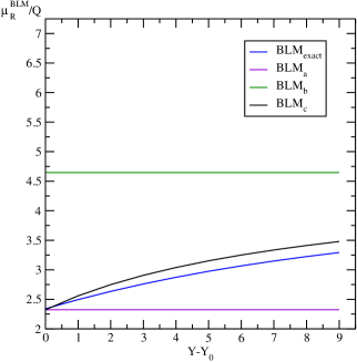
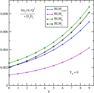
Figure 1: Left: BLM scales for the process $\gamma^{*}\gamma^{*}\to V_{1}V_{2}$ (see the text for details). Right: Forward amplitude for $\gamma^{*}\gamma^{*}\to V_{1}V_{2}$ at $Y_{0}=0$.

Here we present numerical results for the forward amplitude obtained with the BLM optimization method described above.

We consider the case of equal values of photons virtualities, $Q_{1}=Q_{2}=Q$, and, following the first of Refs. [15], present our numerical predictions for the forward amplitude multiplied by some kinematic factors, ${\rm Im}_{s}\left({\cal A}\right)Q^{2}/(sD_{1}D_{2})$, calculated at $Q=50$ GeV, where the expressions for $D_{1,2}$ are given in Eq. (14) of the first of Refs. [15].

For the considered process only the $n=0$ term contributes and the $f(\nu)$ function is given in (34). We will try all approaches to the BLM scale setting described in previous section. In particular, for this process the product of two LO impact factors $c_{1}(n,\nu)c_{2}(n,\nu)$ vanishes very fast for $|\nu|>1$, therefore in the relevant integration $\nu$-range, $|\nu|<1$, we can find the solution of Eq. (46) and determine the BLM scale $\mu_{R,c}^{\rm BLM}$ as a function of $\nu$ and energy.

In Fig. 1(left) we show the values of the BLM to kinematic scale ratios, $\mu_{R}^{\rm BLM}/Q$, as functions of $Y-Y_{0}$, obtained in four different cases. By “exact” case we denote the scale obtained solving numerically Eq. (40) for each value of $\ln\left(s/s_{0}\right)\equiv Y-Y_{0}$. In the other three approaches, the BLM scales depend on $\nu$: the scales for cases $(a)$ and $(b)$ are given by Eqs. (42) and (44), respectively; the case $(c)$ corresponds to the numerical solution of Eq. (46) for each values of $\nu$ and $Y-Y_{0}$. The $\nu$-dependent scales, cases $(a)$, $(b)$ and $(c)$ are shown in Fig. 1(left) for the particular value of $\nu=0$.

Approximate approaches to the scale setting give energy-independent BLM scales (see cases $(a)$ and $(b)$ in Fig. 1(left)), whereas an exact implementation of the BLM rule leads in general to the scales which depend on the energy of the process (see cases $(c)$ and “exact” in Fig. 1(left)). In fact, the approaches $(a)$ and $(b)$ can be considered as a low- and a high-energy approximation to the case $(c)$, where the BLM scale setting prescription is implemented precisely.

Nevertheless, as we already mentioned above, the condition (46) could not be resolved for all processes. Therefore we defined also a method which could be universally applied and which we call here “exact”. It gives a $\nu$-independent BLM scale and it is based on the requirement of vanishing of the integral in Eq. (40), contrary to the approach $(c)$, where we try to make vanish the integrand of the same equation for each separate value of $\nu$.

In Fig. 1(right) we show our predictions as functions of the energy for the forward amplitude calculated with all the four different methods described above: cases $(a)$ and $(b)$ were calculated using Eqs. (43) and (45), cases $(c)$ and “exact” using Eq. (41) with the corresponding choices of the scales. The result of the BFKL resummation depends not only on the renormalization scale $\mu_{R}$, which is fixed here with the BLM method, but also on the energy scale $s_{0}$ or $Y_{0}$. In Fig. 1(right) we present the results obtained with the choice of this scale dictated by the kinematic of the process, $s_{0}=Q^{2}$ or $Y_{0}=0$. A more reliable estimation could result from fixing the value of $Y_{0}$ according to some optimization method, such as PMS, but this goes beyond the scope of present paper.

As we can see in Fig. 1(right), our predictions obtained with precise implementations of BLM method lie inbetween those derived with the use of the two approximate realizations. Note that the difference between the two explicit methods, cases $(c)$ and “exact”, is sizeable and increases with the energy. This is related to the fact that these two approaches are not equivalent, and the scales in the case $(c)$ are larger than those in the “exact” one. Note also that, with the growth of energy, the value of $\nu=\bar{\nu}$ where the solution of Eq. (46) has a singularity decreases, see Eq. (47), and approaches the $\nu$-range important for the determination of our observable.

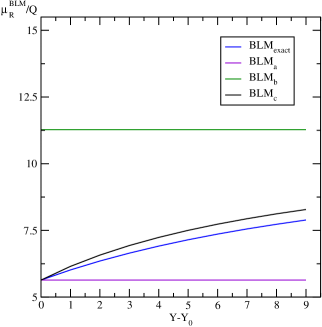
Figure 2: BLM scales for the process $\gamma^{*}\gamma^{*}\to X$ (see the text for details).

4.2 $\gamma^{*}\gamma^{*}$ total cross section

In [26] some of us studied the $\gamma^{*}\gamma^{*}$ total cross section in the NLA BFKL approach considering two different optimization methods of the perturbative series. One of them was the BLM method, cases $(a)$ and $(b)$, described above, where the Eqs. (43) and (45) were transformed back to $\overline{\rm MS}$ scheme. In that paper we fixed the photon virtualities and, correspondingly, the number of active flavors $n_{f}$ in order to make a comparison with LEP2 experimental data. Here, we are interested in the general features of the BLM scale setting procedure, therefore we prefer to fix the photon virtualities as in the two-meson production: $Q_{1}=Q_{2}\equiv Q=50$ GeV with $n_{f}=5$.

In Fig. 2, as in the case of the vector mesons, we show the four different ratios $\mu_{R}^{\rm BLM}/Q$ versus $Y-Y_{0}$. The four cases $(a)$, $(b)$, $(c)$ and “exact” are defined exactly as in the previous subsection. As we mentioned before, cases $(a)$ and $(b)$ are independent on the energy of the process, but depend on the kind of process through the $f(\nu)$ function. In particular, for the production of a pair of light vector mesons the function is given by Eq. (34), while for this process it is $f(\nu)=0$ (see Eq. (33)).

For this process we only discuss here the BLM scale setting and do not present its cross section. The $\gamma^{*}\gamma^{*}$ cross section was already considered in [26], where serious problems were found, related with the very large values of NLO corrections [27] for the virtual photon impact factor. For details and an extended discussion of this issue, we refer the reader to [26].

4.3 Mueller-Navelet jets

The last semihard process that we consider is the production of two forward high-$p_{T}$ jets produced with a large separation in rapidity $\Delta y$ (Mueller-Navelet jets [28]). Such process was studied at Large Hadron Collider (LHC): the CMS collaboration provided with data for azimuthal decorrelations [29] that can be expressed, from a theoretical point of view, by ratios ${\cal{C}}_{m}/{\cal{C}}_{n}$, where ${\cal{C}}_{n}$ are to be averaged over $k_{J_{i}}$ (jet transverse momentum) and $y_{J_{i}}$ (rapidity jet). Then, in order to match the kinematic cuts used by the CMS collaboration, we have

$$C_{n}=\int_{y_{1,\rm min}}^{y_{1,\rm max}}dy_{1}\int_{y_{2,\rm min}}^{y_{2,\rm max}}dy_{2}\int_{k_{J_{1},\rm min}}^{\infty}dk_{J_{1}}\int_{k_{J_{2},\rm min}}^{\infty}dk_{J_{2}}\delta\left(y_{1}-y_{2}-Y\right){\cal C}_{n}\left(y_{J_{1}},y_{J_{2}},k_{J_{1}},k_{J_{2}}\right)\;,$$ (49)

with $y_{1,\rm min}=y_{2,\rm min}=-4.7$, $y_{1,\rm max}=y_{2,\rm max}=4.7$  and $k_{J_{1},\rm min}=k_{J_{2},\rm min}=35$ GeV. The comparison between experimental results for jets with cone radius $R=0.5$ produced at a center-of-mass energy of $\sqrt{s}=7$ TeV and theoretical calculations was done in [31], where the exact NLO impact factors calculated in [32] were used, and in [30], where the NLO impact factors were taken in the small-cone approximation as calculated in [33] .

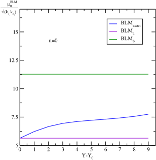
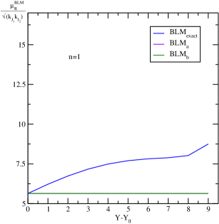
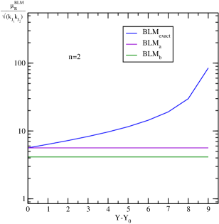
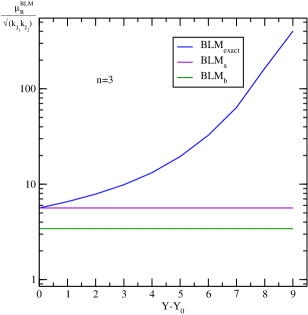
Figure 3: BLM scales for Mueller-Navelet jets (see the text for details).

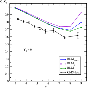
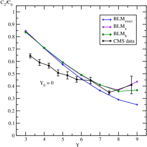
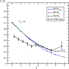
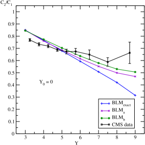
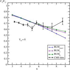
Figure 4: Azimuthal decorrelations for Mueller-Navelet jets (see the text for details).

In this section we use the same kinematic settings as in [30] and present the BLM scale setting for the Mueller-Navelet jet production. In particular, we consider the ratios $\mu_{R}^{\rm BLM}/\sqrt{k_{J_{1}}k_{J_{2}}}$ as functions of $Y-Y_{0}$ for $n$=0, 1, 2 and 3 and recall that, for this process, the function $f(\nu)=0$ is zero. The results are shown in Fig. 3 were the three lines, violet, green and blue, denote the cases $(a)$, $(b)$ and “exact”, respectively. For this process it is not possible to consider the case $(c)$ because the product of LO impact factors $c_{1}(n,\nu)c_{2}(n,\nu)$ is a function that does not decreases so fast, so that the $\nu$-interval needed for the integration includes the value $\overline{\nu}$, defined by Eq. (47), where the method is not applicable.

Due to the integration over the jet variables $k_{J_{1,2}}$ and $y_{J_{1,2}}$, the derivation of the “exact” curve here is a little bit different from that of the other two processes. In this case, in order to get the ratios $\mu_{R}^{\rm BLM}/\sqrt{k_{J_{1}}k_{J_{2}}}$, we write $\mu_{R}=m_{R}\sqrt{k_{J_{1}}k_{J_{2}}}$ and we look for $m_{R}$ such that Eq. (40) is satisfied.

On the contrary, since cases $(a)$ and $(b)$ are independent of the energy of the process for $n=0$, the two curves, “BLM_a” and “BLM_b” are equivalent to those in Fig. 2, since also in the present case $f(\nu)=0$. Moreover, note that, for $n=1$, $\chi(n=1,\nu=0)=0$ and therefore in Fig. 3 the curve “BLM_b” overlaps exactly the curve “BLM_a”.

In Fig. 4 we present some ratios $C_{m}/C_{n}$ versus $Y$, where we make use of the scales shown in Fig. 3. In all cases shown in Fig. 4 the factorization scale $\mu_{F}$ entering the MSTW2008nlo [35] parton distribution functions was chosen equal to the renormalization scale $\mu_{R}$ and the BFKL energy scale $Y_{0}$ was fixed at zero. One could look for optimal choices of the scale $Y_{0}$, based on the PMS method, for instance, but this goes beyond the scope of the present paper. The results shown in [30] are a little bit different from those shown here, because there we transferred back all formulas to the $\overline{\rm MS}$ scheme. Moreover note that now we have an extra-curve (BLM_exact) in which $\mu_{R}$ was obtained solving Eq. (40).

5 Summary

In this paper we have focused on the BLM method to set the renormalization scale in a generic semihard process, as described in the NLA BFKL approach in the $(\nu,n)$-representation. We found that the BLM scale setting procedure is well defined in the context of semihard processes described by the BFKL approach within NLA accuracy. The straightforward application of the BLM procedure leads to a condition to be fulfilled, Eq. (40), which defines the optimal renormalization scale depending on the specific process and on its energy. Our main observation here is that, due to the presence of $\beta_{0}$-terms in the next-to-leading expressions for the process dependent impact factors, the optimal renormalization scale is not universal, but turns out to depend both on the energy and on the type of process in question. The non-universality of the BLM scale setting in exclusive processes was observed already in [36].

Note that the above-mentioned $\sim\beta_{0}$-contributions to NLA impact factors are universally expressed in terms of the LO impact factors of the considered process, see our Eqs. (29) and (3). Thus, they could be easily calculated for all processes, even in the case when the full expressions for the NLO corrections to the impact factors are not known. Such contributions must be taken into account in the implementation of BLM method to the description of cross sections of semihard processes, because all contributions to the cross section that are $\sim\beta_{0}$ must vanish at the BLM scale.

Such an “exact” implementation of the BLM method could be difficult since it calls for the solution of an integral equation, Eq. (40), for each value of the energy of the process. This equation can be solved, in general, only in numerical way. Therefore, we considered several approximated approaches to the BLM scale setting. One of them, the closest to the “exact” one and labeled $(c)$, consists in imposing the vanishing of the integrand appearing in the above-mentioned general condition and leads to an optimal BLM scale depending also on the $\nu$-variable. This approximated method has a validity domain in the $\nu$-space and can be applied only if the relevant range of the $\nu$-integration giving a physical observable falls inside this validity domain. Other approximated approaches, labeled $(a)$ and $(b)$, can be viewed as a sort of low- and high-energy approximation of the case $(c)$ and of the “exact” determination.

We have compared these different approaches in the study of the total cross section and of other physical observables related with the forward amplitude in processes such as the electroproduction of two light vector mesons, the total cross section of two virtual photons and the production of Mueller-Navelet jets . Note that the formulas for the approximate cases $(a)$ and $(b)$ were already used by us, without derivation, in our recent papers [26, 30]. Here we presented in full details the implementation of the BLM method for arbitrary semihard processes, considering both its exact and approximate forms.

We could observe that, in general, the BLM scale setting in the cases $(a)$ and $(b)$ provides with a range inside which lie the “exact” the case $(c)$ determinations. This is not the case for the Mueller-Navelet jet production where, as discussed in the text, due to some peculiarities in the definition of the observables imposed by the experimental cuts, the natural ordering between the optimal scales in the cases $(a)$, $(b)$ and “exact” is sometimes lost. It turns out, however, that azimuthal correlations and ratios between them in the Mueller-Navelet case are less sensitive to the different approaches to BLM scale setting than in the other two processes considered in this work.

Note that previous applications of the BLM method to the description of $\gamma^{*}\gamma^{*}$ total cross sections [37, 38, 7, 39] relied on the use of LO expressions for the photon impact factors. In [37, 38] the $\gamma^{*}\gamma^{*}$ total cross section was considered in LLA BFKL, since the NLO corrections to the BFKL kernel were not yet known. However, in [37, 38] the $\beta_{0}$-part of the first correction to the Born amplitude (i.e. the $t$-channel two-gluon exchange) was considered in order to establish the renormalization scale. Such approach to the scale setting is closely related to our case $(a)$ (scale fixed from the correction to the impact factor). Indeed, considering the expansion of the BFKL amplitude (26), one can see that the first, $\sim\alpha_{s}$, correction to the Born amplitudes originates entirely from NLO parts of the impact factors. Comparing Eq. (5.5) in [38] with our Eq. (42) for $f(\nu)=0$, as appropriate for the $\gamma^{*}\gamma^{*}$ process, one can see that they agree except for the term that, in our approach, derived from the change to the MOM scheme. One can therefore refer to [37, 38] as to the first (approximate) application of the BLM scale setting to a BFKL calculation. In [7, 39] the $\gamma^{*}\gamma^{*}$ total cross was considered using full NLA BFKL kernel, but with LO approximation for the photon impact factor. In respect with the BLM scale setting, such approach is equivalent to our approximate case $(b)$.

In [31] the BLM method was applied to Mueller-Navelet jet production: although the full NLO expression for the jet impact factor was used, the above-discussed effect of $\beta_{0}$-contributions to NLO jet impact factors on the choice of the BLM scale was overlooked. Therefore in [31] the value of the BLM scale which was obtained is similar to the one used in [7, 39] and, as such, coincides with our approximate case $(b)$. Our results presented in Fig. 4 allow to assess the inaccuracy in BLM predictions for different Mueller-Navelet jet observables related with approximated approaches to the BLM scale setting.

In conclusion, the BLM method for scale setting, which was proposed more than three decades ago on a strong physical basis, remains a fundamental tool for perturbative calculations and has lead to many successful comparisons between theoretical predictions and experimental data. In this paper we have provided with the general paradigm for its systematic application to an important class of processes, i.e. semihard processes within the NLA BFKL approach, thus filling some gaps left open by previous approximated or incomplete approaches. We believe that this will increase the future significance of the method.

References

- [1] V.S. Fadin, E.A. Kuraev, L.N. Lipatov, Phys. Lett. B 60 (1975) 50; E.A. Kuraev, L.N. Lipatov and V.S. Fadin, Zh. Eksp. Teor. Fiz. 71 (1976) 840 [Sov. Phys. JETP 44 (1976) 443]; 72 (1977) 377 [45 (1977) 199]; Ya.Ya. Balitskii and L.N. Lipatov, Sov. J. Nucl. Phys. 28 (1978) 822.
- [2] V.S. Fadin and L.N. Lipatov, Phys. Lett. B 429 (1998) 127 [hep-ph/9802290]; M. Ciafaloni and G. Camici, Phys. Lett. B 430 (1998) 349 [hep-ph/9803389].
- [3] L.N. Lipatov, V.S. Fadin, Sov. J. Nucl. Phys. 50 (1989) 712; V.S. Fadin and R. Fiore, Phys. Lett. B 294 (1992) 286; V.S. Fadin and L.N. Lipatov, Nucl. Phys. B 406 (1993) 259; V.S. Fadin, R. Fiore and A. Quartarolo, Phys. Rev. D 50 (1994) 5893 [hep-th/9405127]; V.S. Fadin, R. Fiore and M.I. Kotsky, Phys. Lett. B 359 (1995) 181; V.S. Fadin, R. Fiore and M.I. Kotsky, Phys. Lett. B 387 (1996) 593 [hep-ph/9605357]; V.S. Fadin, R. Fiore, M.I. Kotsky, Phys. Lett. B 389 (1996) 737 [hep-ph/9608229]; V.S. Fadin, R. Fiore and A. Quartarolo, Phys. Rev. D 53 (1996) 2729 [hep-ph/9506432]; V.S. Fadin, L.N. Lipatov, Nucl. Phys. B 477 (1996) 767 [hep-ph/9602287]; V.S. Fadin, M.I. Kotsky and L.N. Lipatov, Phys. Lett. B 415 (1997) 97; V.S. Fadin, R. Fiore, A. Flachi, M.I. Kotsky, Phys. Lett. B 422 (1998) 287 [hep-ph/9711427]; S. Catani, M. Ciafaloni and F. Hautmann, Phys. Lett. B 242 (1990) 97; G. Camici and M. Ciafaloni, Phys. Lett. B 386 (1996) 341 [hep-ph/9606427]; Nucl. Phys. B 496 (1997) 305 [hep-ph/9701303].
- [4] V.S. Fadin, hep-ph/9807528.
- [5] S.J. Brodsky, G.P. Lepage, P.B. Mackenzie, Phys. Rev. D 28 (1983) 228.
- [6] S.J. Brodsky, V.S. Fadin, V.T. Kim, L.N. Lipatov and G.B. Pivovarov, JETP Lett. 70 (1999) 155 [arXiv:hep-ph/9901229].
- [7] S.J. Brodsky, V.S. Fadin, V.T. Kim, L.N. Lipatov and G.B. Pivovarov, JETP Lett. 76 (2002) 249 [Pisma Zh. Eksp. Teor. Fiz. 76 (2002) 306] [arXiv:hep-ph/0207297].
- [8] S.V. Mikhailov, JHEP 0706 (2007) 009 [hep-ph/0411397].
- [9] S.J. Brodsky and X.G. Wu, Phys. Rev. D 85 (2012) 034038 [arXiv:1111.6175 [hep-ph]]; Phys. Rev. D 85 (2012) 114040 [arXiv:1205.1232 [hep-ph]]; Phys. Rev. D 86 (2012) 014021 [arXiv:1204.1405 [hep-ph]]; Phys. Rev. Lett. 109 (2012) 042002 [arXiv:1203.5312 [hep-ph]; S.J. Brodsky and L.D. Giustino, Phys. Rev. D 86 (2012) 085026 [arXiv:1107.0338 [hep-ph]]; M. Mojaza, S.J. Brodsky and X.G. Wu, Phys. Rev. Lett. 110 (2013) 192001 [arXiv:1212.0049 [hep-ph]]; S.J. Brodsky, M. Mojaza and X.G. Wu, Phys. Rev. D 89 (2014) 1, 014027 [arXiv:1304.4631 [hep-ph]].
- [10] X.G. Wu, S.J. Brodsky and M. Mojaza, Prog. Part. Nucl. Phys. 72 (2013) 44 [arXiv:1302.0599 [hep-ph]].
- [11] X.G. Wu, Y. Ma, S.Q. Wang, H.B. Fu, H.H. Ma, S.J. Brodsky and M. Mojaza, arXiv:1405.3196 [hep-ph]].
- [12] A.L. Kataev, arXiv:1411.2257 [hep-ph].
- [13] A.L. Kataev and S.V. Mikhailov, Phys. Rev. D 91 (2015) 1, 014007 [arXiv:1408.0122 [hep-ph]].
- [14] H.H. Ma, X.G. Wu, Y. Ma, S.J. Brodsky and M. Mojaza, arXiv:1504.01260 [hep-ph].
- [15] D.Yu. Ivanov and A. Papa, Nucl. Phys. B 732 (2006) 183 [hep-ph/0508162]; Eur. Phys. J. C 49 (2007) 947 [hep-ph/0610042]; F. Caporale, A. Papa and A. Sabio Vera, Eur. Phys. J. C 53 (2008) 525 [arXiv:0707.4100 [hep-ph]].
- [16] A.V. Kotikov and L.N. Lipatov, Nucl. Phys. B 582 (2000) 19 [hep-ph/0004008].
- [17] A.V. Kotikov and L.N. Lipatov, Nucl. Phys. B 661 (2003) 19 [Erratum-ibid. B 685 (2004) 405] [hep-ph/0208220].
- [18] V.S. Fadin, D.Yu. Ivanov and M. I. Kotsky, Phys. Atom. Nucl. 65 (2002) 1513 [Yad. Fiz. 65 (2002) 1551] [hep-ph/0106099].
- [19] D.Yu. Ivanov and A. Papa, JHEP 1207 (2012) 045 [arXiv:1205.6068 [hep-ph]].
- [20] B. Pire, L. Szymanowski and S. Wallon, Eur. Phys. J. C 44 (2005) 545 [hep-ph/0507038].
- [21] M. Segond, L. Szymanowski and S. Wallon, Eur. Phys. J. C 52 (2007) 93 [hep-ph/0703166 [hep-ph]].
- [22] V.P. Goncalves and W.K. Sauter, Phys. Rev. D 73 (2006) 077502 [hep-ph/0601072].
- [23] R. Enberg, B. Pire, L. Szymanowski and S. Wallon, Eur. Phys. J. C 45 (2006) 759 [Erratum-ibid. C 51 (2007) 1015] [hep-ph/0508134].
- [24] D.Yu. Ivanov, M.I. Kotsky and A. Papa, Eur. Phys. J. C 38 (2004) 195 [hep-ph/0405297].
- [25] P.M. Stevenson, Phys. Lett. B 100 (1981) 61; Phys. Rev. D 23 (1981) 2916.
- [26] D.Yu. Ivanov, B. Murdaca and A. Papa, JHEP 1410 (2014) 58 [arXiv:1407.8447 [hep-ph]].
- [27] I. Balitsky and G.A. Chirilli, Phys. Rev. D 87 (2013) 1, 014013 [arXiv:1207.3844 [hep-ph]].
- [28] A.H. Mueller, H. Navelet, Nucl. Phys. B 282 (1987) 727.
- [29] CMS Collaboration, S. Chatrchyan et al., CMS PAS FSQ-12-002.
- [30] F. Caporale, D.Yu. Ivanov, B. Murdaca and A. Papa, Eur. Phys. J. C 74 (2014) 3084 [arXiv:1407.8431 [hep-ph]].
- [31] B. Ducloué, L. Szymanowski and S. Wallon, Phys. Rev. Lett. 112 (2014) 082003 [arXiv:1309.3229 [hep-ph]].
- [32] J. Bartels, D. Colferai and G.P. Vacca, Eur. Phys. J. C 24 (2002) 83 [hep-ph/0112283]; Eur. Phys. J. C 29 (2003) 235 [hep-ph/0206290]; F. Caporale, D.Yu Ivanov, B. Murdaca, A. Papa and A. Perri, JHEP 1202 (2012) 101 [arXiv:1112.3752 [hep-ph]].
- [33] D.Yu Ivanov and A. Papa, JHEP 1205 (2012) 086 [arXiv:1202.1082 [hep-ph]].
- [34] D. Colferai and A. Niccoli, arXiv:1501.07442 [hep-ph].
- [35] A.D. Martin, W.J. Stirling, R.S. Thorne and G. Watt, Eur. Phys. J. C 63 (2009) 189 [arXiv:0901.0002 [hep-ph]].
- [36] I.V. Anikin, B. Pire, L. Szymanowski, O.V. Teryaev and S. Wallon, Eur. Phys. J. C 42 (2005) 163 [hep-ph/0411408].
- [37] S.J. Brodsky, F. Hautmann and D.E. Soper, Phys. Rev. Lett. 78 (1997) 803 [Phys. Rev. Lett. 79 (1997) 3544] [hep-ph/9610260].
- [38] S.J. Brodsky, F. Hautmann and D.E. Soper, Phys. Rev. D 56 (1997) 6957 [hep-ph/9706427].
- [39] X.C. Zheng, X.G. Wu, S.Q. Wang, J.M. Shen and Q.L. Zhang, JHEP 1310 (2013) 117 [arXiv:1308.2381 [hep-ph]].