Fast functional integrals with application to differential equations models
1. Abstract
A new method is introduced which uses higher-order Laplace approximation to evaluate functional integrals much faster than existing methods. An implementation in MATLAB is called SLAM-FIT (Sparse Laplace Approximation Method for Functional Integration on Time) or simply SLAM. In this paper SLAM is applied to estimate parameters of mixed models that require functional integration. It is compared with two more general packages which can be used to do functional integration. One is Stan, a recent and very general package for integrating and estimating using hybrid Monte Carlo. The other is INLA, a recent R package which uses Laplace approximations for Gaussian Markov random fields. In both cases it is able to get near-identical or equivalent results in less time for moderately sized data sets. The fundamental speed advantage of the algorithm may be greater than it appears, because SLAM is running in pure MATLAB while the other two packages use optimized compiled code.
Keywords: compartment models, predator-prey, SIR model, path integral, functional integral, Laplace approximation, saddlepoint method.
2. Introduction
This paper has two purposes: to introduce a new, much faster computational method for functional integration, and to show its usefulness in estimating parameters of differential equation models. For a time-dependent random process, a functional integral can be thought of as the integral over all possible values at all times over the relevant time interval (Dirac, 1933; Feynman and Hibbs, 2010; Schulman, 2005; Kleinert, 2009). Technically they are integrals over a function space such as a space of Brownian motion paths. They have been used for at least eighty years in many branches of science and applied mathematics including quantum and statistical mechanics, polymer science, probability, and finance. Typically they are used to compute the chance of a system evolving from one state to a different one: any in-between path is possible, but the probability is given by the integral over the possible paths. This makes them a natural tool to use for analyzing systems which are imperfectly modeled by ordinary differential equations. In life science there are predator-prey models (Edelstein-Keshet, 1988), infectious disease models (Kermack and McKendrick, 1927; Anderson and May, 1991), pharmacokinetics models (Gelman et al., 1996), and many others. Most of macroeconomics depends on differential equation-based models such as the Solow growth model or the ISLM model (Romer, 2011). These models can be made more realistic by considering noise or stochastic behavior.
A major goal of differential equations models is to estimate system parameters, such as how infectious a virus is, or reaction rates for chemicals and enzymes. Traditional approaches involve simplified models on transformed variables (Lineweaver and Burk, 1934) or optimizing some measure of data fit over exact solutions to the ODEs (Anderson and May, 1991). Recent methods use a generalized smoothing approach. For a finite-dimensional basis, such as splines, it is possible to approximately fit both the differential equations and the data (Ramsay J. et al., 2007; Campbell and Steele, 2012). As with smoothing, the trade-off between data fit and ODE fit can be chosen by cross-validation or by a mixed-model approach.
In this paper, we use a very different approach: we discretize time, and model the underlying true values as a first-order Markov process. Then we assume that the data were generated with a distribution depending on the true value. Not all of the time points have data; in fact, it may be important to add in-between time points, just as they would be needed for a finite difference method. Then we define a marginalized pseudolikelihood of the system parameters as an integral over the possible values which the variables might have taken at the time points. This approximates a functional integral over a continuous random process.
There are both analytic and computational methods for evaluating functional integrals. Analytic methods require a tractable integrand or a good approximation to one. Very clever schemes have been painstakingly developed to transform functional integrals and make them tractable (Kleinert, 2009; Schulman, 2005). Far more problems have so far required time-consuming Monte Carlo methods.
Laplace and saddlepoint approximations have also been used to approximate analytic functional integrals when possible. But this appears to be the first time that the approximations have been used for numerical evaluation. One reason for this may be that some of the higher-order terms, involving third- and fourth-order tensors, are difficult to evaluate efficiently.
This paper introduces a way to compute the higher-order terms quickly for numerical functional integrals. This requires computing a critical path (a unique most likely realization) and expanding the log-likelihood around it. The log-likelihood is a sum of interactions between neighboring time points. Consequently the relevant Hessian and the tensors of third- and fourth-order derivatives are sparse with a simple block structure: all entries corresponding to non-neighboring time points are zero. By using this sparsity structure, it is possible to calculate the higher-order terms in time, where is the number of time points and is the number of variables in the system.
A variance-stabilizing transformation is needed when the data times are separated by many in-between time steps. In general it makes the integrals more accurate than when untransformed. SLAM can be used with the basic Laplace term alone, or with the higher-order terms. Higher-order terms make the integrals more accurate, but for the examples tested, the parameter estimates are close to those found using the basic Laplace approximation.
To evaluate speed and accuracy, SLAM was compared with two popular systems for mixed models. Results for an infectious disease data set are equivalent to results from Stan (STAN Development Team, ), the leading general-purpose Monte Carlo system, but SLAM is much faster. There is also a well-implemented Laplace-based method, INLA (Rue et al., 2009, ), designed for hierarchical models and Gaussian Markov random fields.
For random fields, INLA takes advantage of sparsity, but the higher-order terms still take quadratic time. The special approximation introduced here can only be applied to GMRFs on a line, not for other type covered by INLA. To compare INLA and SLAM, we used an INLA demonstration data set (Tokyo rainfall by day of year). For repeats of the Tokyo data, estimates are well within the CI for the two methods. INLA (with full higher-order terms) is faster at 1100 data points but SLAM is faster beyond that. INLA using simplified higher-order terms remains somewhat faster up to the largest set tested (about 15000 data points).
3. METHODS
3.1. Markov process setup
The model has two stages: a Markov process for the true values, and on top of that, measurements with noise. We assume that the Markov and measurement likelihoods depend on parameters . We show how to define a marginalized likelihood for . Maximizing the marginalized likelihood gives an estimate of .
In this paper we will use Latin indexes (“i”) to denote time points and matrix blocks. We use Greek indexes (“”) to denote individual vector and matrix entries. Each time point has as one entry for every variable. This becomes important when analyzing the blocking structure. We also use the summation convention for duplicated indexes (e.g. means .)
The Markov process has a vector value at each time point, denoted by at step (time ). (We use without an index to mean the entire realization, i.e., the concatenation of the .) The system also has parameters that involved in the Markov process or the measurement error. From the Markov process, at time there is a conditional probability density for , given the value of :
so given the initial values , we have the overall conditional density for a realization at all time points:
If we have a prior we can define the probability of a realization:
Some of the time points have data. Let be the set of their indexes. Call the data values for . We assume that the data are independently generated with a probability density depending on the true value and parameters:
Depending on the system, the error could be measurement error from an instrument, or from sampling error, or from some other source. The overall density of the given realization and data is
This means that the pdf of given is given by
Given it is possible to define a marginal likelihood for by integrating over the latent true values. But in general, we don’t know , and we use the improper prior . The integral is finite because of the multiplication by which can be thought of as a prior on the data points. This gives us the marginalized pseudolikelihood
where
This marginalized pseudolikelihood is what we will maximize to estimate .
3.2. Laplace approximation (basic and higher-order)
In this subsection, we look closely at how to get a good approximation for . In addition, assume that has a single peak at . Then we can expand around :
where is the Hessian of at , and and are the tensors of third and fourth derivatives at .
We can think of as a Gaussian random variable, with precision matrix , and this integral is the expectation of a function of :
The expectation can be expanded and then approximated with an asymptotic series.
This series diverges, but the terms shown can produce a good approximation to on their own. A similar, often better approximation is given by a cumulant expansion for (Shun and McCullagh, 1995; McCullagh, 1987), where the first higher-order terms are the same as above, but the product is turned into a sum:
where
We use the cumulant expansion, for , because the derivatives are simpler and because in many cases it is more accurate (Shun and McCullagh, 1995).
Terms IIIa and IIIb involve the same tensors, but the sums are very different. In term IIIa, as long as we have the near-diagonal entries of , we can immediately convert the third-order tensors into vectors . Then . In section 4 we explain how to compute the near-diagonal entries in time (Asif and Moura, 2005); getting is even faster because is block-tridiagonal.
Term IIIb is different and much more difficult. Each connects one mode of the first to a mode of the second , and is full. This means that entries from one time point of the first are multiplied by entries from all other time points in the second , not just entries from the neighboring time points. This would seem to mean that IIIb requires quadratic time (in ) to compute. The appendix shows how it can be done in linear time by using power series and recurrence relations.
Graphically, the difference can be represented this way:
Here each line represents a contraction over two modes: one from each tensor, if there are two, or two from a single tensor. This notation will be helpful later when doing more complicated manipulations on term IIIb.
It is worth emphasizing that all three of these terms are invariant under linear transformations. If we make a change of variables , then
and the derivatives tensors (at the critical path) become
Then the sum is still equal to term IV, is still term IIIa, etc. In the simplified matrix and graphical notation, the transformation of and can be written as
In reality, both tensors are being multiplied symmetrically in all modes. The reason for using transposes is because if a matrix is on the left side, its rows are multiplied, and if a matrix is on the right side, its columns are multiplied. This is consistent with the usual direction of matrix multiplication. Using the same convention will make things simpler in the Appendix.
4. The Sparsity Structure and How to Use It
Take another look at the log likelihood (3.1). Each term in uses values from one time point. Each term in uses values from two adjacent time points.
This means that if is any time point, the blocks , , and can be nonzero. For any other , i.e. if , . Such a matrix is called block-tridiagonal (see figure 2).
Likewise, is zero unless . And is zero if any of the differences is greater than 1.
4.1. Setup, block-diagonals, block off-diagonals, levels
In this subsection we see how to work with , then apply that to computing and . The details for are worked out in the appendix.
If is a true local minimum of , then has to be positive definite. This is crucial, because we need the Cholesky decomposition for the calculation.
Here is block-diagonal but not symmetric. In fact, is lower-triangular. is block off-diagonal, level -1. This means that can only be nonzero if .
In general, the matrix is block off-diagonal, level , if the blocks only when .
Block-off-diagonals have a raising and lowering property, demonstrated in Figure 2. If is block off-diagonal with level , and is block off-diagonal with level , then is block off-diagonal with level . “Raising the level by 1” happens when you multiply on either size by a block off-diagonal matrix of level 1. “Lowering by 1” is the same as “raising by -1”, which means multiplying by a block off-diagonal of level -1.
If has level , and has level , then has level . The third block of level is zero because has only 2 nonzero blocks.
4.2. Computing near-diagonal elements of
Moving on with the computation,
The power series for actually terminates because is strictly lower-triangular. So we can expand and group terms:
The terms of the double sum can be grouped by level so as to give us the near-diagonal levels of . This results in an algorithm similar to the block-tridiagonal case of (Asif and Moura, 2005).
Each term in the double sum has exactly one level, . Now we will group the terms by level. Break the sum into the two cases, and :
where
Now we will show how to compute in time by a block matrix recurrence relation.
Obviously,
The map has a special property: each block of only depends on the following block of , and the last block of is zero.
Because of this property, we can solve by a reverse iteration:
for going from down to 1.
This gives a total of block multiplications, each of which takes up to flops for total complexity . There may be special cases when there are less than flops per block, but that would be somewhat unusual because is generated by a Cholesky decomposition.
Having computed , we now have
We will never actually compute all the entries of – it is full and would need too many flops. For terms IV and IIIa, we only need the block-tridiagonal part,
which has entries and takes time to compute.
4.3. Computing IV and IIIa
Term IV is simple: each nonzero element of occurs exactly once, and is multiplied by block-tridiagonal elements of . has nonzero terms, and the number of operations is clearly bounded by . It may be less if the blocks of are themselves sparse.
Term IIIa is slightly more complicated. The first part is comparable to term IV: each nonzero element of occurs once. This takes up to time and returns a vector with . Then term IIIa is proportional to . Solving takes time since is triangular and block-banded.
5. Numerical Examples and Experiments
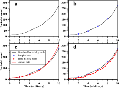
5.1. An Example: Poisson-Distributed Growth and the Need for Variance Stabilization
Imagine a bacteria colony with a known rate of division per minute, . The deterministic equation of growth would be
But we know that the process is not really deterministic, and that the bacteria count and number of divisions are integers. So a reasonable model is that the number of divisions over the short time is Poisson distributed with mean :
But SLAM can’t handle discrete variables directly: the Laplace approximation uses an integral over the values of the . The obvious fix is to use the normal approximation to the Poisson distribution:
where is the data-based likelihood of given . For now we assume that it peaks at .
Now we should be able to find the critical path that minimizes , take derivatives, and compute the various Laplace terms. And presumably, for small enough time steps, this would give a good approximation to the stochastic differential equation.
Unfortunately, without a further tweak, even this simple example can fail precisely because of using small time steps between the data points. If there are too many consecutive time points between the data times, i.e. too many points without data, you can get the problem shown in figure 3. Increasing tends to drive lower and lower; if there are enough points between data points, can approach zero for some time points.
This doesn’t just mean that the critical paths get ugly; they are actually getting farther and farther from any realistic paths that the system might take. This is possible because the probability density of the path is large for close to zero, even though the total probability measure of that region is still quite small. The problem stops being good for a Laplace-type approach.
Fortunately, there is a way around this problem. We start by identifying the reason for it, then explain the solution for this example.
The explanation below is a heuristic, not a theorem, but it is based on actual observation. Rearranging the expression for , we get
The first term is constant with respect to and does not affect the minimization of . The next term is a data term: it only depends on at the data points, and it actually increases when goes below from . So to understand the evolution of the critical path with increasing , we have to look to the other two terms.
The third term (the term) typically increases without bound as . For example, if there is a limiting path , with evenly spaced time points, where is the mean of .
But the last term does not increase without bound. In practice,
behaves like a Riemann sum approaching its limiting value–an integral. This is because, in practice, for small, . (If all of the critical paths were along the same smooth function , then would be . This doesn’t happen here because the come from critical paths for different partitions. Essentially this sum behaves more like it would for a Brownian motion than for a smooth function.)
Using , we get
if the are uniformly bounded below (uniformly for different ).
For this reason, as , the log-likelihood is dominated by the third term, the sum over values of . This is why the critical path keeps being pushed lower and lower in order to minimize .
This creates a problem: for accuracy with a continuous process, we may need small time steps, but with small time steps we get this artifact. It arises because the variance of depends on : a smaller gives a smaller variance, which gives a greater likelihood.
The solution is to make a change of variables in the integral. If we pick the right transformation , we can stabilize the variance of and get a realistic critical path to expand around. If , and is small,
so we can stabilize the variance of if
So has stable variance. How does this affect the integral for ?
If we let
then
and the marginalized likelihood is proportional to
is always positive, so . is maximized when . There is an additional factor of , but realistically it cannot go to infinity as fast as and go to zero for large .
That means that this integrand, unlike the pre-transformation integrand, is bounded and has some reasonable critical path in terms of .
5.2. SIR model
Our primary model for testing comes from infectious disease epidemiology. One of the simplest widely-used models is the SIR model (Kermack and McKendrick, 1927). There are three compartments, Susceptibles, Infected, and Recovered. At each time step, some Susceptibles become Infected, and some Infected become Recovered. Two parameters correspond to infectiousness () and speed of recovery (). The traditional method of estimating these parameters uses the deterministic equations
The assumptions behind this are simple:
(1) new infections are proportional to contacts between susceptible and infected;
(2) new recoveries are proportional to the number infected.
Assumption (2) is memoryless, which is not very realistic, but is often adequate (Anderson and May, 1991).
To convert this to a stochastic model, we treat new infections at time () and new recoveries at time () as independent Poisson variables with means given by the deterministic model:
As with the bacterial colony, we use the normal approximation:
We assume the measurement error is lognormal with a third parameter, :
The dynamical part of the likelihood is
| where | |||
| so | |||
As with the bacteria model §5.1, the critical path often gets artifacts for small time steps and the approximation can be poor. So we rewrite the differential as
so we want to pick transformed variables and such that
If we take
then our integral avoids the artifacts explained in §5.1.
5.3. Comparison with Rstan on British Boarding School data
Stan (STAN Development Team, ) is a tool for doing Bayesian statistics using Hybrid Monte Carlo estimation. Among other things, it can estimate Bayesian posteriors for parameters in very general models, which can be specified with an easy-to-use general model language.
This makes Stan a natural check for the approximation methods in SLAM. The probabilistic model in §5.2 was defined in Stan as well as SLAM, and used to estimate parameters for a classic data set (Murray, 2002). The purpose is to verify that the estimates comes out similar, but that SLAM can make the calculations more quickly because of the approximation. The posterior median given by Stan is not identical to the maximum marginalized likelihood estimate given by SLAM. However, for small variances, we expect them to be close.
The results are shown in the table below along with the corresponding results from SLAM. The test data set comes from an influenza infection at a British boarding school (Murray, 2002). Initial guesses for and are set equal to Murray’s deterministic estimates. The initial guess for (the measurement error parameter) is arbitrarily set to 0.1.
Figure 4 shows the estimates of the course of infection given by SLAM, Stan, and the deterministic ODEs, given their estimated parameter values. The deterministic model suggests that the epidemic could not end as quickly as it did. Stan and SLAM can follow the data more closely using the stochastic model from §5.2. The Stan and SLAM paths are very similar, but we don’t expect them to be identical because Stan is showing posterior means while SLAM is showing a overall maximum likelihood estimate.
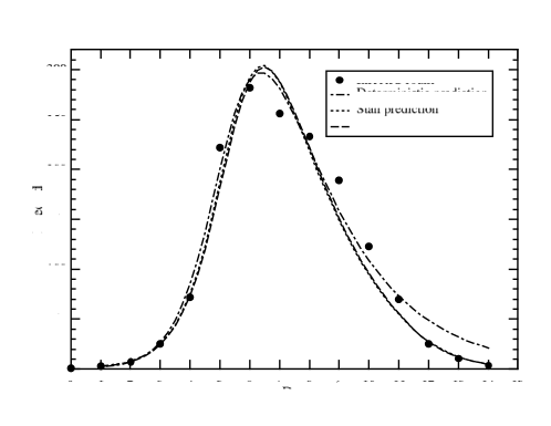
Table 1 shows the results of the test. As expected, the parameter estimates from Stan and SLAM are very similar. For and , the differences are negligible. For the Stan and SLAM estimates are within a fraction of the CI, or about 10% of the value. But for this problem, compared with Stan, basic SLAM was about 35 times faster than Stan, and higher-order SLAM was more than 13 times faster.
| Time | ||||||
| Deterministic (Murray) | 0.440 | – | ||||
| Stan CI Low | 0.462 | 0.092 | ||||
| Stan posterior median | 0.518 | 0.194 | 61.3 | |||
| SLAM basic | 0.519 | 0.175 | 1.7 | |||
| SLAM higher order | 0.519 | 0.176 | 4.5 | |||
| Stan CI High | 0.601 | 0.400 |
For this test, Rstan 2.8.0 was run in R 3.2.2, using 4 chains of length 2000 each, with options set to maximize speed (multicore, optimized compilation). Different versions of Stan code for the model were tested. Surprisingly, the fastest version used unvectorized code.
5.4. Comparison with INLA on Tokyo rain data
INLA (Rue et al., 2009, ) is an R package which also uses Laplace approximations to compute integrals and estimate parameters, but for a different class of problems (Gaussian Markov Random Fields (Rue and Held, 2005)). GMRFs on a line can be analyzed by both INLA and SLAM. INLA also uses sparsity, but the higher-order terms are calculated in a simpler (and more general) way which takes quadratic time and memory in the number of nodes. Therefore SLAM, with a linear-time algorithm for the higher-order terms, should be faster for sufficiently large GMRFs on a line. These experiments show that this is true for repeats of the Tokyo data set (Martino and Rue, 2009) from the INLA package.
The Tokyo data set looks at Tokyo rainfall from the start of 1983 to the end of 1984. Each row of Tokyo gives a calendar day (e.g. January 28) and the number of times it rained on that day in either 1983 or 1984. For obvious reasons this count is always 2 except for February 29 (from 1984). The top few rows are presented in Table 2.
| i | ||
|---|---|---|
| 1 | 2 | 0 |
| 2 | 2 | 0 |
| 3 | 2 | 1 |
| 4 | 2 | 1 |
| 5 | 2 | 0 |
Here is the calendar date (e.g. 1 is January 1), is the number of times that date occurred, and is the number of rain days for that date.
In the INLA manual (Martino and Rue, 2009), the Tokyo data set is analyzed using INLA with a second-order random walk model ( Rue and Held (2005), section 3.4.1). For each date , the chance of rain is assumed to be some , so the chance of rain days for that date is . The second-order random walk is over , so for given is
After slight modifications111Three modifications were made in order to work around features that are not yet present in the SLAM code. 1. SLAM doesn’t take second derivatives, so an extra variable is added which is forced to be nearly equal to the true . Then the usual RW2 penalty is given in terms of . 2. INLA has an option “cyclic” which forces the function to be periodic. SLAM does not currently have such an option. Therefore cyclic is set to FALSE for INLA. Happily, the predicted functions are nearly periodic. 3. The Tokyo data set covers 1983-84, so for all dates except February 29. For Feb. 29 because only 1984 was a leap year. For now, it was necessary to set for February 29 for both programs. Think of it as a recording error. we compared the behavior and performance of INLA and SLAM.
In order to adjust the size of the data set, we simply repeated the data set k times, e.g., for k=2 there are 732 data points instead of 366 and .
By default, INLA uses an approximation to the higher order terms which is easier to compute (strategy=‘simplified.laplace’). To get the full higher order Laplace terms, as used by SLAM, we set INLA strategy = ‘laplace’.
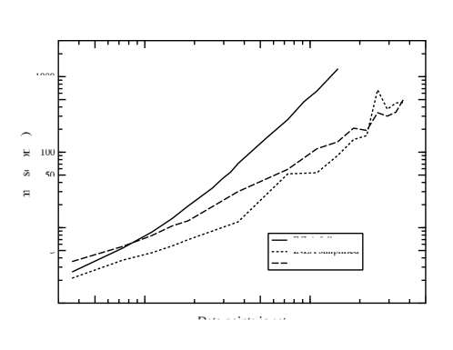
After running both packages on Tokyo, the estimates are not identical but are very similar, especially for the larger data sets (see figures). The most important results here have to do with run time and especially memory use. For k up to 3, INLA is faster. At k=4 (), SLAM becomes faster. The relative difference grows as shown in figure 6.
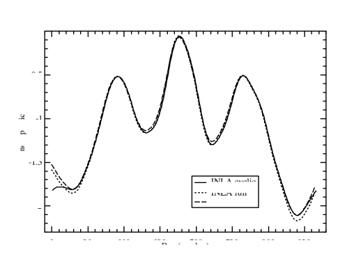
The SSE for the simplified Laplace is several times larger than for INLA full or for SLAM. This is almost entirely due to greater error near the ends of the year (1 and 366).
The expected number of rain days over the year is and the observed number of rain days is . For SLAM these are equal to at least four digits. This probably means that, under some conditions, the method forces them to be equal. For now we make no suggestion why.
Lastly, in this example we had to introduce a variable which is supposed to be the time derivative of the linear predictor . We forced to be close to the true derivative by adding a large penalty for any difference between and . These results show that it is (sometimes) possible to use SLAM for a constrained system using this simple trick.
6. Discussion
We have shown how to efficiently compute a higher-order Laplace approximation for functional integrals on time. This can be used to define a marginalized pseudolikelihood for differential equation systems involving randomness. In turn, these approximate marginalized likelihoods can be maximized in order to estimate parameters of the system, such as infectiousness of a disease, or a good roughness parameter for a smoothing problem. This approximation is implemented in the MATLAB package SLAM. SLAM is compared on real data against two leading packages which also estimate/predict parameters according to a fully Bayesian system or mixed model. As predicted, the time needed for SLAM seems to grow linearly. Compared with either package, for medium-sized data sets using higher-order terms, SLAM produces equivalent results in far less time. This is especially interesting given that both Stan and INLA use compiled, optimized code. Finally, for some problems, if higher-order terms are used then SLAM is able to process significantly larger data sets than INLA.
7. Acknowledgements
This work was begun at the Center on Aging and Health, Johns Hopkins Bloomberg School of Public Health, under Training Grant T32AG000247 (Epidemiology and Biostatistics of Aging). Additional support was provided by the Biostatistics Department at JHSPH. I would like to thank Alan Cohen (now at Sherbrooke University) for inviting me into the project which led to this. I would also like to thank Ravi Varadhan and Giles Hooker for consultation and encouragement, and Karen Bandeen-Roche for making it possible. Michael Schumaker provided help with editing and LaTeX. Thanks are also due to the developers of Stan, INLA, and the MATLAB Tensor Toolbox for quick and friendly answers to my questions.
8. Appendix: Calculation of Term IIIb in linear time
8.1. Tensor levels
This shows how to compute term IIIb in time. This is possible because of the raising and lowering principle described in section 4. A similar concept applies to block tensors. A tensor of order 3, , is block off-diagonal with level if every nonzero block has . In other words, is level if it is block off-diagonal and includes the block . Levels are an equivalence class: level is the same as level for any integer .
The levels of a third-order block tensor are shifted when powers of or are applied to the modes. Our is a sum of a handful of block-diagonal and block off-diagonal levels. To compute IIIb, we find the combinations of powers of and which connect the levels of the first with the levels of the second . The grouping is more complicated than for computing the near-diagonals of , but is similar in spirit.
Suppose have a single-level matrix and a single-level tensor with level . If is level , then the new tensor is also block off-diagonal, but with level . The next observation is critical: if is applied to every mode of , the result is the same exact level as .
8.2. A simplifying coordinate transformation
As we discussed in section 8, we can write term IIIb more simply by making a coordinate transformation:
where
is block-diagonal with block size , so the coordinate transformation takes time.
To continue, we will use the series
We simplify this by making a second block-diagonal coordinate transformation to eliminate . Note that is block-diagonal and symmetric because each of its terms is block-diagonal and symmetric. is also positive definite, since is positive definite and every is semidefinite. So if we define to be the (upper!) Cholesky decomposition . Then , and . Now we can make the coordinate transformation
from which
The first and third terms are transposes of each other. Let’s look at the first term alone.
with . At last,
where .
8.3. Statement of Results
where
and is defined as
can be computed in time, and so can the whole sum.
8.4. How to expand the sum and group the terms
Let’s start by defining a more compact notation.
This has the properties of multilinearity and symmetry under permutation:
Furthermore, if all the matrices are transposed, then you get the same value:
Multilinearity and permutation symmetry mean that we can expand our bracket of sums in the same way as with a product of sums.
Combining transposes lets us group the terms together further:
The calculation of is trivial: it’s just . The other two involve grouping the tiny minority of nonzero subterms in the first two terms. The principle to remember is that none of the nonzero levels are more than two apart in any of the 3 modes. This means that if any of are more than 2, and if either or is greater than 2. Taking the middle term first,
All terms have power . But this implies that the only nonzero terms have . If were greater than 1, we would have . for similar reasons. And if were greater than 1 we would have . Consequently, this triply-infinite sum reduces to
Finally, we reach the first sum, which is also the most complicated:
Using
then these terms become
Putting the whole expression together,
Like the computation in near-diags there is a simple, linear recurrence relation for . First, solves a linear equation:
In block notation, this gives us a recurrence relation similar to LABEL:Solving_S. This is a forward recurrence instead of backwards because of
The recurrence is forward instead of backward because we chose to use rather than for the main sum. Each successive block of is computed in terms of a known block of and (if present) the previous block of from the same level. There are 7 block levels, the number of blocks per level is , and the number of operations in a matrix-times-block operation is , so the complexity of finding is .
The computation can be accelerated by separating the levels of and making greater use of symmetry, but it will still be .
References
- Anderson and May [1991] R. Anderson and R. May. Infectious Diseases of Humans: Dynamics and Control. Oxford University Press, Oxford, UK, 1991.
- Asif and Moura [2005] A. Asif and J.M.F. Moura. Block matrices with L-block-banded inverse: inversion algorithms. IEEE Transactions on Signal Processing, 53(2):630–642, 2005.
- Campbell and Steele [2012] D. Campbell and R.J. Steele. Smooth functional tempering for nonlinear differential equation models. Statistics and Computing, 22(2):429–443, 2012.
- Dirac [1933] P. Dirac. The Lagrangian in quantum mechanics. Physikalische Zeitschrift der Sowjetunion, 3:64–72, 1933.
- Edelstein-Keshet [1988] L. Edelstein-Keshet. Mathematical Models in Biology. Random House, New York, NY, USA, 1988.
- Feynman and Hibbs [2010] R. P. Feynman and A. R. Hibbs. Quantum Mechanics and Path Integrals. Dover, 2010. (Original published in 1965).
- Gelman et al. [1996] A. Gelman, F. Bois, and J. Jiang. Physiological pharmacokinetic analysis using population modeling and informative prior distributions. J. Am. Statist. Ass., 91(436):1400–1412, 1996.
- Kermack and McKendrick [1927] W. O. Kermack and A. G. McKendrick. A contribution to the mathematical theory of epidemics. Proc. Roy. Soc. Lond. A, 115(772):700–721, 1927.
- Kleinert [2009] H. Kleinert. Path Integrals in Quantum Mechanics, Statistics, Polymer Physics, and Financial Markets. World Scientific, 5th edition, 2009. Individual chapters available at http://users.physik.fu-berlin.de/ kleinert.
- Lineweaver and Burk [1934] H Lineweaver and D. Burk. The determination of enzyme dissociation constants. Journal of the American Chemical Society, 56(3), 1934.
- Martino and Rue [2009] S. Martino and H. Rue. INLA manual. 2009. Available at http://www.math.ntnu.no/ hrue/GMRFsim/manual.pdf.
- McCullagh [1987] P. McCullagh. Tensor Methods in Statistics. Chapman & Hall, London, UK, and New York, NY, USA, 1987.
- Murray [2002] J.D. Murray. Mathematical Biology I, An Introduction. Springer-Verlag, 2002.
- Ramsay J. et al. [2007] Hooker G.J. Ramsay J. et al. Parameter estimation for differential equations: a generalized smoothing approach. Journal of the Royal Statistical Society B, 69:741–796, 2007.
- Romer [2011] D. Romer. Advanced Macroeconomics. McGraw-Hill, Columbus, OH, USA, 4th edition, 2011.
- Rue and Held [2005] H. Rue and L. Held. Gaussian Markov Random Fields: Theory and Applications. Chapman & Hall, 2005.
- Rue et al. [2009] H. Rue, S. Martino, and N. Chopin. Approximate Bayesian inference for latent Gaussian models by using integrated nested Laplace approximations. J. R. Statist. Soc. B, 71(2):319–392, 2009.
- [18] H. Rue et al. The r-inla project. http://www.r-inla.org.
- Schulman [2005] L. S. Schulman. Techniques and Applications of Path Integration. Dover, 2005. Reprint of 1981 version.
- Shun and McCullagh [1995] Z. Shun and P. McCullagh. Laplace Approximation of high dimensional integrals. J. R. Statist. Soc. B, 57(4):749–760, 1995.
- [21] STAN Development Team. STAN: A C++ Library for Probability and Sampling, Version 2.1. STAN, 2013. http://mc-stan.org.