$D^{+}\rightarrow K^{-}\pi^{+}\pi^{+}$ - the weak vector current

Abstract

Studies of D and B mesons decays into hadrons have been used to test the standard model in the last fifteen years. A heavy meson decay involves the combined effects of a primary weak vertex and subsequent hadronic final state interactions, which determine the shapes of Dalitz plots. The fact that final products involve light mesons indicates that the QCD vacuum is an active part of the problem. This makes the description of these processes rather involved and, in spite of its importance, phenomenological analyses tend to rely on crude models. Our group produced, some time ago, a schematic calculation of the decay $D^{+}\rightarrow K^{-}\pi^{+}\pi^{+}$, which provided a reasonable description of data. Its main assumption was the dominance of the weak vector-current, which yields a non-factorizable interaction. Here we refine that calculation by including the correct momentum dependence of the weak vertex and extending the energy ranges of $\pi\pi$ and $K\pi$ subamplitudes present into the problem. These new features make the present treatment more realistic and bring theory closer to data.

I motivation

Non-perturbative QCD calculations are difficult and can only be performed in approximate frameworks. The grouping of quarks into two sets, according to their masses, provides a convenient point of departure for approximations. Quarks $u$, $d$, and $s$ can be considered as light and quarks $c$, $b$, and $t$, as heavy, even though the $s$-quark is not too light and the $c$-quark is not too heavy. This approach is useful because light quark condensates are active close to the ground state of QCD and give rise to highly collective interactions.

Pions and kaons are the most prominent light quark systems, but data available for elastic $K\pi$ scattering are scarce and decades old. They were obtained from the LASS spectrometer at SLACLASS ; Estab , in the range $0.825<\sqrt{s}<1.960$ GeV, by isolating one-pion exchanges in the reaction $KN\to\pi KN$. In the last ten years, information about $K\pi$ interactions was also produced by hadronic decays of $D$ mesons. In particular, data from the E791 and FOCUS collaborationsE791kappa ; FOCUS for the reaction $D^{+}\to K^{-}\pi^{+}\pi^{+}$ allowed the $S$-wave $K\pi$ sub-amplitude to be extracted continuously from threshold up to the high energy border of the Dalitz plot. Hope was then raised that these data could improve the description of elastic $K\pi$ scattering. However, decay data differ significantly from those given by the LASS experiment and this discrepancy motivates our interest in this problem.

The description of the decay $D^{+}\to K^{-}\pi^{+}\pi^{+}$ must include both the weak $c\rightarrow s$ vertex and hadronic final state interactions (FSIs), which correspond to strong processes occurring between primary decay and detection. The study of weak vertices departs from the topological structures given by ChaoChao , which implement CKM quark mixing for processes involving a single $W\,$. As primary decays occur in the presence of light quark condensates, the direct incorporation of Chao’s scheme into calculations is not trivial and one is forced into hadronic descriptions. These include both the use of form factors in weak vertices, as in the work of Bauer, Stich and WirbelBSW , and the treatment of relativistic final state interactions. High-energy few-body calculations begin to be available nowAzimov ; lc09 ; Zhou and several works have already employed field theory to FSIs in heavy meson decaysCa ; Bo ; Me ; Jap ; DeD ; DiogoRafael ; BR ; satoshi .

In this work, the decay $D^{+}\to K^{-}\pi^{+}\pi^{+}$ is treated by means of chiral effective lagrangians, supplemented by phenomenological form factors. This framework is motivated by the smallness of the $u\,$, $d\,$, and $s$ masses, when compared with the QCD scale $\Lambda\sim 1\,$GeV. The light sector of the theory is therefore not far from the massless limit, which is symmetric under the chiral $SU(3)\times SU(3)$ flavour group. In this approach, light condensates arise naturally and pseudoscalar mesons are described as Goldstone bosons. Quark masses are incorporated perturbatively into effective lagrangiansWchi ; GL , whereas weak interactions are treated as external sources. Chiral perturbation theory was originally designed to describe low-energy interactions, where it yields the most reliable representation of QCD available at present. Its scope was later enlarged, with the inclusion of resonances as chiral correctionsEGPR , and the unitary ressummation of diagramsOO . Suitable coupling schemes also allow the incorporation of heavy mesonsHM .

A similar theoretical framework has already been employed by our groupBR , in an exploratory study of FSIs in $D^{+}\rightarrow K^{-}\pi^{+}\pi^{+}$. With the purpose of taming an involved calculation, in that work we made a number of simplifying assumptions. Among them, the weak vertices were taken to be constants, isospin $3/2$ and $P$ waves were not included in intermediate $K\pi$ amplitudes, and couplings to either vector mesons or inelastic channels were neglected. In spite of these limitations, that work allowed the identification of leading dynamical mechanisms and gave rise to results which are reasonable for the modulus and good for the phase of the $S$-wave $K\pi$ sub-amplitudeE791kappa ; FOCUS . In this work, we focus on the vector weak amplitude and improve the description of the weak vertex, by including both the correct momentum dependence and better phenomenology for an intermediate $\pi\pi$ subamplitude, and the description of a $K\pi$ subamplitude at higher energies. These new features tend to reduce the gap between theory and experiment.

II dynamics

We denote by $[K^{-}\pi^{+}]_{S}$, the $S$-wave $K^{-}\pi^{+}$ sub-amplitude in the decay $D^{+}\rightarrow K^{-}\pi^{+}\pi^{+}$, which has been extracted by the E791E791kappa and FOCUSFOCUS collaborations. The decay begins with the primary quark transition $c\rightarrow s\;W^{+}$, which is subsequently dressed into hadrons, owing to the surrounding light quark condensate. In the absence of form factors, this structure gives rise to the colour allowed process shown in Fig.1, where $a$ and $b$ involve an axial current and $c$ contains a vector current. As one of the pions in diagram $c$ is neutral, it does not contribute at tree level.

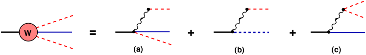
Figure 1: Topologies for the weak vertex: the dotted line is a scalar resonance and the wavy line is the $W^{+}$, which is contracted to a point in calculations.

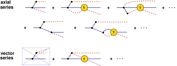
Figure 2: Final state interactions starting from the axial weak vertex (axial series ) and from the vector weak vertex (vector series); in the former, the pion plugged to the $W^{+}$ is always positive, whereas the $\bar{K}$ inside the loop can be either positive or neutral; in the latter, the tree diagram does not contribute, since one of the pions plugged to the $W^{+}$ is neutral.

Inclusion of final state interactions, due to successive elastic $K\pi$ scatteringsBR , yields three families of diagrams, as in Figs.2. It is worth noting that these series do not represent a loop expansion, because loops are also present within the $K\pi$ amplitude. The $W^{+}$ is shown explicitly, just to indicate the various topologies, and becomes point-like in calculations. A family of FSIs endows the forward propagating resonance in Fig.1b with a dynamical widthDiogo . Processes involving resonances have already been considered in Refs.DeD ; Jap ; satoshi , whereas quasi two-body axial FSIs were discussed Ref.DiogoRafael . An important lesson drawn from our previous studyBR is that, for some yet unknown reason, the vector weak amplitude, represented by diagram $(c)$ of Fig.1, seems to be favoured by dataFOCUS . This amplitude receives no contribution at tree level, since the $W^{+}$ emitted by the $c$-quark decays into a $\pi^{+}\pi^{0}$ pair. Therefore, leading terms in this process necessarily involve loops, which bring imaginary components into the amplitude.

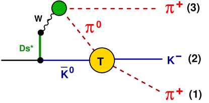
Figure 3: Leading vector current contribution, dressed by form factors and $\pi\pi$ interactions (in the small green blob).

The first non-vanishing contribution to the vector series is given in Fig.3. As the $W$ is very heavy, one keeps just hadronic propagators, which render loop integrals finite. Denoting by $A_{0}$ the amplitude for the process $D^{+}\to K^{0}\pi^{0}\pi^{+}$ without FSIs and by $T_{K\pi}$ that for $\pi^{0}\bar{K}^{0}\to\pi^{+}K^{-}$, the amplitude $A_{1}$ of Fig.3 can be schematically written as

$$A_{1}=-i\int\frac{d^{4}\ell}{(2\pi)^{4}}\;T_{K\pi}^{S}\,\Delta_{\pi}\,\Delta_{K}\;A_{0}\;,$$ (1)

where $\ell$ is the loop variable and $\Delta_{\pi}$ and $\Delta_{K}$ are pion and kaon propagators.

The amplitude $A_{0}$ is described in App.B. The $D\rightarrow W\bar{K}$ vertex includes $D_{s}^{*}$ intermediate states, associated with form factors parametrized in terms of nearest pole dominance weakFF and could be a vector or a scalar. The $W\rightarrow\pi\pi$ form factor is shown in Fig.4 and includes the $\rho$, with a dynamical width. The bare resonance is treated employing the formalism developed in Ref.EGPR and its width is constructed using the $P$-wave elastic $\pi\pi$ amplitude. The $W\rightarrow\pi\pi$ form factor is time-like and its inclusion into the vector series of Fig.2 can, in principle, give rise to final state interactions depending on both $\pi\pi$ and $K\pi$ amplitudes. With the purpose of keeping complications to a minimum, we consider just $\pi\pi$ interactions which are contiguous to the $W$ and occur to the left of the first $K\pi$ amplitude.

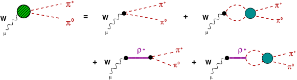
Figure 4: Structure of the $W\rightarrow\pi\pi$ form factor; the blue blob is the elastic $\pi\pi$ amplitude.

The evaluation of Fig.3 requires the $K\pi$ amplitude in the interval $0.401\,$GeV${}^{2}\leq s\leq 2.993\,$GeV². As LASS dataLASS begins only at $s=0.681\,$GeV², one covers the low-energy region by means of theoretical amplitudes, based on unitarized chiral symmetryEGPR . Our intermediate $S$-wave $K\pi$ amplitude, denoted by $T_{K\pi}^{S}$, is thoroughly discussed in App.C.

Using results $(\ref{B.17})$ into eq.$(\ref{2.1})$, one finds

$$A_{1}^{S}(m_{12}^{2}) \!=\! -\,i\,\left[G_{F}\,\cos^{2}\theta_{C}\,F_{1}^{DK}(0)\right]\;\left[\frac{\sqrt{2}}{3}\,T_{K\pi}^{S}(m_{12}^{2})\right]\int\frac{d^{4}\ell}{(2\pi)^{4}}\;\frac{1}{D_{\pi}\,D_{K}}\;\frac{m_{\rho}^{2}}{D_{\rho}}$$ (2)

$$\!\times\! \left\{[M_{D}^{2}\!+\!2M_{\pi}^{2}\!+\!M_{K}^{2}\!-\!2m_{12}^{2}\!-\!\ell^{2}\!+\!D_{\pi}\!+\!D_{K}\,]\,\frac{m_{V}^{2}}{D_{V}}\right.$$

$$\!+\! \left.D_{\pi}\,(M_{D}^{2}\!-\!M_{K}^{2})\left[\frac{1}{D_{V}}-\frac{1}{D_{S}}\right]\right\}\;,$$

where $G_{F}$ is the Fermi constant, $\theta_{C}$ is the Cabibbo angle, $F_{1}^{DK}(0)$ is a coupling constantweakFF , the factor $\sqrt{2}/3$ is associated with the transition $K^{0}\pi^{0}\rightarrow K^{-}\pi^{+}$, whereas $D_{\pi}=[(\ell\!-\!p_{3})^{2}\!-\!M_{\pi}^{2}]$, $D_{K}=[(\ell\!-\!P)^{2}\!-\!M_{K}^{2}]$, $D_{V}=[\ell^{2}\!-\!m_{V}^{2}]$, $D_{S}=[\ell^{2}\!-\!m_{S}^{2}]$, in which the subscripts $V$ and $S$ stand for the $D_{s}^{*}(2112)$ and $D_{s0}^{*}(2317)$ states. Finally, $D_{\rho}$ is a complex function defined by eqs.(36) and (37). This structure yields

$$A_{1}^{S}(m_{12}^{2}) \!=\! -i\,\alpha\,\frac{\sqrt{2}}{3}\,\left[\frac{T_{K\pi}^{S}(m_{12}^{2})}{16\pi^{2}}\right]\left\{\;\beta\,I_{\pi K\rho V}^{S}-I_{\pi KV}^{S}+I_{\pi\rho V}^{S}+I_{K\rho V}^{S}-\gamma\,I_{K\rho VS}^{S}\right\}\;,$$ (3)

with

$$\alpha \!=\! \left[G_{F}\,\cos^{2}\theta_{C}\,F_{1}^{DK}(0)\right]\;m_{\rho}^{2}\,m_{V}^{2}\;,$$ (4)

$$\beta \!=\! M_{D}^{2}\!+\!2M_{\pi}^{2}\!+\!M_{K}^{2}\!-\!m_{\rho}^{2}\!-\!2m_{12}^{2}\;,$$ (5)

$$\gamma \!=\! -(M_{D}^{2}\!-\!M_{K}^{2})(m_{V}^{2}\!-\!m_{S}^{2})/m_{V}^{2}\;,$$ (6)

and

$$I_{abc}^{S} \!=\! \int\frac{d^{4}\ell}{(2\pi)^{4}}\;\frac{16\pi^{2}}{D_{a}\,D_{b}\,D_{c}}\;,\;\;\;I_{abcd}^{S}=\int\frac{d^{4}\ell}{(2\pi)^{4}}\;\frac{16\pi^{2}}{D_{a}\,D_{b}\,D_{c}\,D_{d}}\;.$$ (7)

The form of these integrals is discussed in App.D.

III vector FSI series

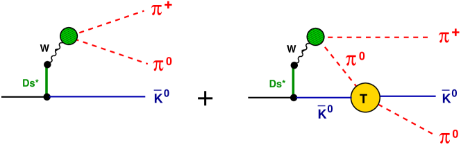
Figure 5: Vector current diagrams contributing to the decay $D^{+}\rightarrow\bar{K}^{0}\pi^{0}\pi^{+}$.

In the decay $D^{+}\rightarrow K^{-}\pi^{+}\pi^{+}$, there is no tree contribution to the vector FSI series, as in Fig.2. However, before moving into this reaction, it is instructive to assess the relative importance of allowed tree and one-loop contributions in the decay $D^{+}\rightarrow\bar{K}^{0}\pi^{0}\pi^{+}$, indicated in Fig.5. The amplitude describing the left diagram is denoted by $A_{0}$ and given in eq.(38). Projecting out the $S$-wave, we find

$$A_{0}^{S} \!=\! -[G_{F}\,\cos^{2}\theta_{C}\,F_{1}(0)]\sum_{i}\left\{\frac{m_{V}^{2}\,N_{i}}{m_{V}^{2}\!-\!\theta_{i}}\right.$$ (8)

$$\!\times\! \left.\left[\left(M_{D}^{2}+2M_{\pi}^{2}+M_{K}^{2}-2m_{12}^{2}-m_{V}^{2}\right)\;\Pi_{V}\right.\right.$$

$$\!-\! \left.\left.\left(M_{D}^{2}+2M_{\pi}^{2}+M_{K}^{2}-2m_{12}^{2}-\theta_{i}\right)\;\Pi_{\theta_{i}}\right]\right\}\;,$$

$$\Pi_{[V;\theta_{i}]} \!=\! \frac{1}{2\,\beta}\;\ln\frac{[\,m_{V}^{2};\,\theta_{i}\,]\!-\!\alpha_{13}^{2}\!-\!\beta\,}{[\,m_{V}^{2};\,\theta\,]\!-\!\alpha_{13}^{2}\!+\!\beta\,}\;,$$ (9)

where $\theta_{i}$ are complex parameters given in table 1 (App.B). The first order amplitude is obtained by replacing the isospin factor $\sqrt{2}/3$ with $-1/3$ in eq.(3) and reads

$$A_{1}^{S}(m_{12}^{2}) \!=\! i\,\alpha\,\frac{1}{3}\,\left[\frac{T_{K\pi}^{S}(m_{12}^{2})}{16\pi^{2}}\right]\left\{\;\beta\,I_{\pi K\rho V}^{S}-I_{\pi KV}^{S}+I_{\pi\rho V}^{S}+I_{K\rho V}^{S}-\gamma\,I_{K\rho VS}^{S}\right\}\;,$$ (10)

Results for the moduli of $A_{0}^{S}$ and $A_{1}^{S}$, displayed in Fig.6, indicate a clear dominance of the former. The main structural difference between both terms is the factor $\left\{T_{K\pi}^{S}/48\pi^{2}\right\}$ in the latter, associated with a final state scattering. Its scale can be understood by noting that chiral symmetry predicts this amplitude to be $T_{K\pi}^{S}=2\,M_{\pi}M_{K}/F^{2}\sim 13$ at threshold whereas LASS data LASS indicate that it reaches a maximum of $T_{K\pi}^{S}\sim 50$ around $m_{12}\sim 1.33\,$GeV. Therefore the factor $\left\{T_{K\pi}^{S}/48\pi^{2}\right\}$ is always smaller than $1/10\,$ and pushes down the loop contribution. This result can be taken as an indication that the vector series, as given in fig.2, converges rapidly. The confirmation of this hint depends, of course, on the explicit calculation of next terms in the series.

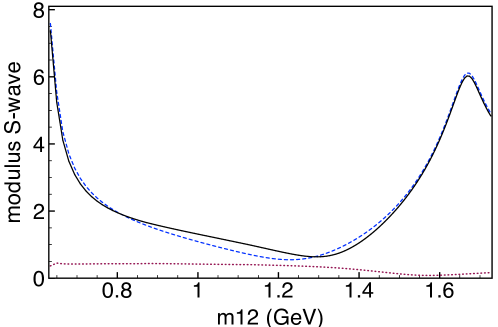
Figure 6: Modulus of the $D^{+}\rightarrow\bar{K}^{0}\pi^{0}\pi^{+}$ amplitude (full line) and partial contributions from eqs.(8) (dashed line) and (10) (dotted line).

IV results - $S$-wave

One of the purposes of this work is to understand the role played by the high energy components of intermediate $\pi\pi$ and $K\pi$ subamplitudes in the description of data. Predictions from eq.(3) for the phase and modulus of $[K^{-}\pi^{+}]_{S}$, the $S$-wave $K^{-}\pi^{+}$ sub-amplitude in $D^{+}\rightarrow K^{-}\pi^{+}\pi^{+}$, are given in Figs.7 and 8.

As far as the $\pi\pi$ subsystem is concerned, the data of Hyams et al.Hyams are used in a parametrized form, in the whole region of interest, as discussed in App.B. For the sake of producing a contrast, we also show curves corresponding to the low-energy vector-meson-dominance approximation, in which the $P$-wave amplitude is described by just an intermediate $\rho$-meson, which amounts to using just the first term in eq.(37). In the case of the $K\pi$ amplitude, data are not available for energies below $0.825\,$GeV LASS and two alternative extensions are given in App.C. One of them is based on a two-resonance fit, which encompasses both low- and high-energy sectors, whereas in the other one LASS dataLASS is used directly, when available, and extrapolated to the threshold region by means of a fit. In the sequence we refer to these versions as fitted and hybrid, respectively. The main difference between them is that the former excludes points around $E\sim 1.7\,$GeV, shown in Fig.11, where two-body unitarity is violated.

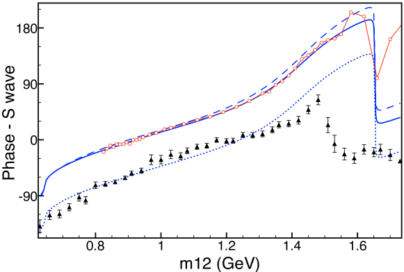
Figure 7: Predictions for $D^{+}\!\rightarrow\!K^{-}\pi^{+}\pi^{+}$ phase (full blue curve), based on the parametrized $\pi\pi$ and $K\pi$ amplitudes given in appendices B and C, compared with FOCUS dataFOCUS ; the blue dotted curve is the previous one shifted by $-55^{0}$; the dashed blue curve is based on one-$\rho$ pole approximation for the $\pi\pi$ amplitude; in the red symbol-continuous curve the hybrid model was used for the $K\pi$ amplitude.

Inspecting the figures, one learns that the improvement in $\pi\pi$ phenomenology is more important for the modulus, where it influences considerably the curve behaviour and increases significantly the range in energy where the theoretical description proves to be reasonable. In the case of the phase, effects associated with $\pi\pi$ phenomenology are small and visible only above $m_{12}>1.2\,$GeV. On the other hand, the use of either the fitted or hybrid $K\pi$ amplitudes produces equivalent results, except at the high energy end, where none of them is satisfactory. This seems to indicate missing structures, that could be associated with other topologies in $D^{+}\!\rightarrow\!K^{-}\pi^{+}\pi^{+}$ decay.

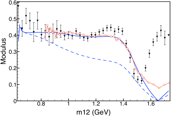
Figure 8: Predictions for $D^{+}\!\rightarrow\!K^{-}\pi^{+}\pi^{+}$ modulus (full blue curve), based on the parametrized $\pi\pi$ and $K\pi$ amplitudes given in appendices B and C, compared with FOCUS dataFOCUS , using arbitrary normalization; the dashed blue curve is based on one-$\rho$ pole approximation for the $\pi\pi$ amplitude; in the red symbol-continuous curve the hybrid model was used for the $K\pi$ amplitude.

As experimental results for the FOCUS phaseFOCUS include an arbitrary constant, in Fig.7 we also show our main result displaced by $-55^{0}$. One notices an overall good agreement with data, from threshold up to $m_{12}\sim 1.4\,$GeV. As our results were based on the vector series shown in Fig.2, which does not contain a tree contribution, there are two sources of complex phases in this problem. One of them is that associated with the $K\pi$ amplitude, whereas the other one is less usual and due to the loop including the weak vertex. Our results indicate that the latter is rather important over the whole energy range considered. This shows the relevance of proper three body interactions, which share the initial momentum with all final particles at once.

V conclusions

In this work we calculate the weak vector current contribution to the process $D^{+}\!\rightarrow\!K^{-}\pi^{+}\pi^{+}$ , employing intermediate $\pi\pi$ and $K\pi$ intermediate sub-amplitudes valid within most of the Dalitz plot. Together with the use of a proper $P-$wave weak vertex, this extends a previous study made on the subjectBR . We still concentrate on $[K^{-}\pi^{+}]_{S}$, the $S$-wave $K^{-}\pi^{+}$ sub-amplitude, and present predictions for both the phase and modulus, given by the blue curves in Figs.7 and 8, are quite satisfactory from threshold to $1.4\,$GeV. Results for the modulus, in particular, improve considerably our previous findings, showing that intermediate $\pi\pi$ subamplitudes are important and need to be treated carefully. As far as the phase is concerned, the most prominent feature is the fact that it has a large negative value at threshold. In QCD, loops are the only source of complex amplitudes and, in this problem, the energy available in the loop of Fig.3 can be larger than both $K\pi$ and $K\rho$ thresholds. This yields a rich complex structure for the loop containing the W, with a phase $\Theta_{L}$ which adds to the phase $\Theta_{K\pi}$ already present in the intermediate $K\pi$ amplitude. Therefore $\Theta_{L}$ represents the gap between the two and three-body phases, which depends on both $m_{12}$ and $m_{23}$, showing that Watson’s theorem does not apply to this case. Our results both confirm the dominance of weak vector currents in this branch of $D^{+}$ decays and indicate that proper three body final-state interactions, in which the initial four-momentum of the $D^{+}$ is shared among all final particles, are rather important over the whole energy range considered. In a parallel study, to be presented elsewhere, we found that this feature is also present in the $P-$wave projection of final-state $K\pi$ subamplitude, which has a non-vanishing phase at threshold.

Appendix A kinematics

The momentum of the $D$-meson is $P\,$, whereas those of the outgoing kaon and pions are $p_{2}\,$, $p_{1}\,$, and $p_{3}\,$, respectively. The invariant masses read

$$m_{12}^{2}=(p_{1}\!+\!p_{2})^{2}=M_{\pi}^{2}+M_{K}^{2}+2\,p_{1}\!\cdot\!p_{2}\;,$$ (11)

$$m_{13}^{2}=(p_{1}\!+\!p_{3})^{2}=2\,M_{\pi}^{2}+2\,p_{1}\!\cdot\!p_{3}\;,$$ (12)

$$m_{23}^{2}=(p_{2}\!+\!p_{3})^{2}=M_{\pi}^{2}+M_{K}^{2}+2\,p_{2}\!\cdot\!p_{3}\;,$$ (13)

and satisfy the constraint

$$M_{D}^{2}=m_{12}^{2}+m_{13}^{2}+m_{23}^{2}-2\,M_{\pi}^{2}-M_{K}^{2}\;.$$ (14)

The projection into partial waves for subsystem $(12)$ is performed by going to its center of mass and writing

$$m_{13}^{2} \!=\! \alpha_{13}^{2}-\beta_{12}\,\cos\theta\;,$$ (15)

$$m_{23}^{2} \!=\! \alpha_{23}^{2}+\beta_{12}\,\cos\theta\;,$$ (16)

$$\alpha_{13}^{2} \!=\! \left[M_{D}^{2}+2\,M_{\pi}^{2}+M_{K}^{2}-m_{12}^{2}-\,(M_{D}^{2}\!-\!M_{\pi}^{2})\,(M_{K}^{2}\!-\!M_{\pi}^{2})/m_{12}^{2}\right]/2\;,$$ (17)

$$\alpha_{23}^{2} \!=\! \left[M_{D}^{2}+2\,M_{\pi}^{2}+M_{K}^{2}-m_{12}^{2}+\,(M_{D}^{2}\!-\!M_{\pi}^{2})\,(M_{K}^{2}\!-\!M_{\pi}^{2})/m_{12}^{2}\right]/2\;,$$ (18)

$$\beta_{12} \!=\! 2\,Q^{\prime}q^{\prime}\;,$$ (19)

$$q^{\prime} \!=\! \frac{1}{2\sqrt{m_{12}^{2}}}\left[m_{12}^{4}-2(M_{\pi}^{2}\!+\!M_{K}^{2})\,m_{12}^{2}+(M_{\pi}^{2}\!-\!M_{K}^{2})^{2}\right]^{1/2}\;,$$ (20)

$$Q^{\prime} \!=\! \frac{1}{2\sqrt{m_{12}^{2}}}\left[m_{12}^{4}-2(M_{\pi}^{2}\!+\!M_{D}^{2})\,m_{12}^{2}+(M_{\pi}^{2}\!-\!M_{D}^{2})^{2}\right]^{1/2}\;,$$ (21)

where $\theta$ is the angle between the momenta of the pions.

Appendix B basic $D^{+}\rightarrow\bar{K}^{0}\pi^{0}\pi^{+}$ amplitude

Our description of the decay $D^{+}\to K^{-}\pi^{+}\pi^{+}$ includes both the primary weak vertex and hadronic final state interactions, associated with successive $K\pi$ scatterings. When the $W\rightarrow\pi\pi$ vertex is corrected by means of time-like form factors, both the $\rho$-meson and $P$-wave $\pi\pi$ interactions also become part of the problem. This could, in principle, give rise to a structure of final interactions depending on both $\pi\pi$ and $K\pi$ amplitudes. For the sake of keeping complications under control, we consider here just $\pi\pi$ interactions which occur to the left of $K\pi$ amplitudes. Therefore, the amplitude for the process $D^{+}(P)\rightarrow\bar{K}^{0}(p_{K})\pi^{0}(p_{0})\pi^{+}(p_{+})$, given in Fig.4 and denoted by $A_{0}$, becomes the basic building block in the evaluation of the weak vector series.

We begin by constructing $T_{\pi\pi}^{P1}$, the isospin $I=1$, $P$-wave $\pi\pi$ amplitude. The momenta of the outgoing pions are $p_{+}$ and $p_{0}\,$, whereas those inside the two-pion loop are $q_{+}$ and $q_{0}$. The total momentum is $Q=(p_{+}+p_{0})=(q_{+}+q_{0})$ and the loop integration variable is $\ell=(q_{+}-q_{-})/2$. Assuming that, at low energies, $\pi\pi$ interactions are dominated by a ${\cal{O}}(q^{2})$ contact term supplemented by the ${\cal{O}}(q^{4})$ $\rho$-pole contribution, the effective lagrangians in Ref.EGPR yield the tree contribution

$$\bar{T}^{1}=(t-u)\left[\frac{1}{F^{2}}-\frac{2\,G_{V}^{2}}{F^{4}}\,\frac{s}{s-m_{\rho}^{2}}\right]\,,$$ (22)

where $F$ is the pion decay constant and $G_{V}$ describes the $\rho\,\pi\pi$ coupling. The approximation $G_{V}=F/\sqrt{2}\sim 66\,$MeV yields a more compact structure, given by

$$\bar{T}^{1}=-\,\frac{(t-u)}{F^{2}}\;\frac{m_{\rho}^{2}}{s-m_{\rho}^{2}}\,.$$ (23)

For free particles in the center of mass frame, $(t-u)=(s-4M_{\pi}^{2})\,\cos\theta$ and $P$-wave projection yields the kernel

$${\cal{K}}^{P1}=-\,\frac{(s-4M_{\pi}^{2})}{3\,F^{2}}\;\frac{m_{\rho}^{2}}{s-m_{\rho}^{2}}$$ (24)

The iteration of this kernel by means of intermediate two-pion states produces the unitarized amplitudeOO

$$T_{\pi\pi}^{P1}=\frac{{\cal{K}}^{P1}}{1+{\cal{K}}^{P1}\,\Omega_{\pi\pi}}\;,$$ (25)

where $\Omega_{\pi\pi}$ is a divergent loop function. Therefore, we write it as the sum of an infinite constant $\Lambda_{\infty}$ and a regular component $\bar{\Omega}_{\pi\pi}\,$, given byBR

$$\bar{\Omega}_{\pi\pi}=-\frac{S}{16\pi^{2}}\,\left\{2-\frac{\sqrt{\lambda}}{s}\;\ln\left[\frac{s-2M_{\pi}^{2}+\sqrt{\lambda}}{2M_{\pi}^{2}}\right]+i\;\pi\;\frac{\sqrt{\lambda}}{s}\right\}\;,$$

$$\lambda=s^{2}-4\,s\,M_{\pi}^{2}\;,$$ (26)

where $S=1/2$ is the symmetry factor for identical particles. After regularization, one finds

$$T_{\pi\pi}^{P1}=\frac{{\cal{K}}^{P1}}{1+{\cal{K}}^{P1}\,(\bar{\Omega}_{\pi\pi}+C_{\pi\pi)}}\;,$$ (27)

where $C_{\pi\pi}$ is an arbitrary constant. This amplitude is related with phase shifts by

$$T_{\pi\pi}^{P1} \!=\! 32\pi\,\left[\frac{s}{s-4M_{\pi}^{2}}\right]^{1/2}\sin\delta\,e^{i\delta}$$ (28)

and we fix $C_{\pi\pi}$ by the phase at $90^{0}\,$. The I=1 amplitude to be used in the evaluation of $A_{0}$ is given by eq.(27) multiplied by $(3\,\cos\theta)$. It is denoted by $T_{\pi\pi}^{1}$ and can be cast in the covariant form

$$T_{\pi\pi}^{1}=3\frac{(t-u)}{s-4M_{\pi}^{2}}\;T_{\pi\pi}^{P1}=-\,6\,\frac{(p_{+}-p_{0})^{\nu}\ell_{\nu}}{s-4M_{\pi}^{2}}\;T_{\pi\pi}^{P1}\;.$$ (29)

Going back to the decay amplitude $A_{0}$ and reading the diagrams in Fig.4, one finds

$$A_{0} \!=\! [G_{F}\,\cos^{2}\theta_{C}]\,\langle\;\bar{K}^{0}|V^{\mu}|D^{+}\;\rangle\,\left[\frac{m_{\rho}^{2}}{Q^{2}\!-\!m_{\rho}^{2}}\right]\left[\,(p_{+}\!-\!p_{0})_{\mu}+i\,6\,\frac{(p_{+}-p_{0})^{\nu}}{Q^{2}-4M_{\pi}^{2}}\;T_{\pi\pi}^{P1}(Q^{2})\;I_{\mu\nu}\right]\,,$$

$$I_{\mu\nu} \!=\! \int\!\frac{d^{4}\ell}{(2\pi)^{4}}\;\frac{\ell_{\mu}\,\ell_{\nu}}{[(\ell\!+\!Q/2)^{2}-M_{\pi}^{2}]\,[(\ell\!-\!Q/2)^{2}-M_{\pi}^{2}]}\,,$$ (30)

where $G_{F}$ is the Fermi constant, $\theta_{C}$ is the Cabibbo angle, $V^{\mu}$ is the weak vector current. The regular part of $I_{\mu\nu}$ can be related with eq.(26) and one hasHR ; PCM

$$I_{\mu\nu}=\frac{i}{6}\left[Q^{2}-4M_{\pi}^{2}\right]\left[g_{\mu\nu}-\frac{Q_{\mu}Q_{\nu}}{Q^{2}}\right]\;[\bar{\Omega}_{\pi\pi}+C_{\pi\pi}]$$ (31)

Using this result into eq.(30) and recalling that $(p_{+}-p_{0})^{\nu}Q_{\nu}=0$ for on shell particles, one has

$$A_{0} \!=\! [G_{F}\,\cos^{2}\theta_{C}]\,\langle\;\bar{K}^{0}|V^{\mu}|D^{+}\;\rangle\;(p_{+}\!-\!p_{0})_{\mu}\;\frac{m_{\rho}^{2}}{D_{\rho}}\;,$$ (32)

$$D_{\rho} \!=\! (Q^{2}\!-\!m_{\rho}^{2})-(m_{\rho}^{2}/3F^{2})\,(Q^{2}\!-\!4M_{\pi}^{2})\,[\,[\bar{\Omega}_{\pi\pi}+C_{\pi\pi}]\;.$$ (33)

The vector current matrix element is written as

$$\langle\;\,\bar{K}^{0}\,|\,V^{\mu}\,|\,D^{+}\,\;\rangle \!=\! \left(P_{D}^{\mu}+p_{K}^{\mu}\right)F_{1}^{DK}(Q^{2})-Q^{\mu}\;\frac{M_{D}^{2}\!-\!M_{K}^{2}}{Q^{2}}\left[F_{1}^{DK}(Q^{2})-F_{0}^{DK}(Q^{2})\right]$$ (34)

and form factors are parametrized in terms of vector and scalar $c\bar{s}$ nearest poles asweakFF

$$F_{1}(Q^{2})=\frac{F^{DK}(0)}{1-Q^{2}/m_{V}^{2}}\hskip 14.22636pt\mathrm{and}\hskip 14.22636ptF_{0}(Q^{2})=\frac{F^{DK}(0)}{1-Q^{2}/m_{S}^{2}}\,,$$ (35)

with $V\rightarrow D_{s}^{*}(2100)$, $S\rightarrow D_{s}^{*}(2317)$ and $F^{DK}(0)=0.75$.

The denominator $D_{\rho}$ describes the $\rho$ meson and includes its dynamically generated width. The function $D_{\rho}$ does not vanish along the real axis, in spite of the bare $\rho$ propagators in Fig.4. It has a zero in the second Riemann sheet, quite close to the value quoted in Ref.CGL , namely at $Q^{2}=(m_{\rho}-i\,\Gamma_{\rho}/2)^{2}\,$, $m_{\rho}=762.4\pm 1.8\,$MeV, $\Gamma_{\rho}=145.2\pm 2.8\,$MeV.

In order to simplify calculations one notes that the ratio $m_{\rho}^{2}/D_{\rho}$ in eq.(32) is related to the $P$-wave amplitude given by eq.(25) by

$$\frac{m_{\rho}^{2}}{D_{\rho}}=-\;\frac{3\,F^{2}}{s-4M_{\pi}^{2}}\;T_{\pi\pi}^{P1}\;.$$ (36)

Using the data from Hyams et al.Hyams , we fitted this ratio using the structure

$$\frac{m_{\rho}^{2}}{D_{\rho}}=\frac{N_{\rho}}{s-\theta_{\rho}}+\frac{N_{1}}{s-\theta_{1}}+\frac{N_{2}}{s-\theta_{2}}\;,$$ (37)

with free parameters $\theta_{k}=\theta_{kR}+i\,\theta_{kI}$ and $N_{k}=N_{kR}+i\,N_{kI}\,$, given in table 1.

$\;\;k\;\;$	$\theta_{R}$	$\theta_{I}$	$N_{R}$	$N_{I}$
$\rho$	0.580133	-0.1137172	0.6131598	-0.1107509
1	2.539625	-0.6468928	0.2418401	-0.1080483
2	3.642091	-0.1595399	0.0016668	-0.1941643

Table 1: Fitted parameters in eq.(37)

.

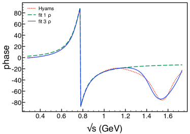
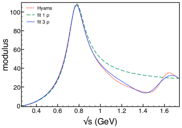
Figure 9: Results for $\pi\pi$ phase and modulo with only one-$\rho$ (dashed) and adding another two poles (continuous), compared with Hyams et al.Hyams (dotted).

In Figs. 9 and 10 we display the importance of the inclusion of higher poles in eq.(37) in extending the agreement with Hyams et. al.Hyams data.

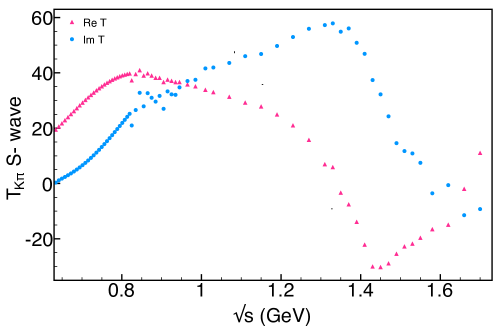
Figure 10: Function $m_{\rho}^{2}/D_{\rho}$; the red continuous curve represents eq.(36) with parameters from Hyams et al.Hyams and the black dotted curve is our fit, using eq.(37); as data begin at $0.6\,$GeV, the red curve to the left of the vertical dashed line corresponds to an extrapolation.

The expression for $A_{0}$ to be used in calculations is obtained by assembling previous results, and one finds

$$A_{0} \!=\! -\,[G_{F}\,\cos^{2}\theta_{C}\,F^{DK}(0)]\,\left[\frac{N_{\rho}}{Q^{2}-\theta_{\rho}}+\frac{N_{1}}{Q^{2}-\theta_{1}}+\frac{N_{2}}{Q^{2}-\theta_{2}}\right]$$ (38)

$$\!\times\! \left\{\left[M_{D}^{2}\!+\!2M_{\pi}^{2}\!+\!M_{K}^{2}-2(p_{0}\!+\!p_{K})^{2}-Q^{2}+(p_{0}^{2}\!-\!M_{\pi}^{2})+(p_{K}^{2}\!-\!M_{K}^{2})\right]\,\frac{m_{V}^{2}}{Q^{2}\!-\!m_{V}^{2}}\right.$$

$$\!-\! \left.(p_{0}^{2}\!-\!M_{\pi}^{2})\,\frac{(M_{D}^{2}\!-\!M_{K}^{2})\,(m_{V}^{2}\!-\!m_{S}^{2})}{(Q^{2}\!-\!m_{V}^{2})\,(Q^{2}\!-\!m_{S}^{2})}\right\}\;.$$

Appendix C $K\pi$ amplitude

In this work, one needs the elastic $K\pi$ amplitude over the full Dalitz plot. As there are no dataLASS available in the interval $0.401\,$GeV${}^{2}\leq s\leq 0.681\,$GeV², one encompasses this region with the help of a theoretical amplitude, based on the unitarized chiral symmetry. This model has been discussed in detail in Ref.BR ; PAT-Kpi and here we just summarize its main features.

For each spin-isospin channel, the unitary amplitude $T_{LI}$ is obtained by ressumming the infinite geometric series

$$T_{LI} \!=\! {\cal{K}}_{LI}-{\cal{K}}_{LI}\,[\bar{\Omega}_{K\pi}\!+\!C_{LI}]\,{\cal{K}}_{LI}+{\cal{K}}_{LI}\,[\bar{\Omega}_{K\pi}\!+\!C_{LI}]\,{\cal{K}}_{LI}\,[\bar{\Omega}_{K\pi}\!+\!C_{LI}]\,{\cal{K}}_{LI}+\cdots$$ (39)

$$\!=\! \frac{{\cal{K}}_{LI}}{1+[\bar{\Omega}_{K\pi}\!+\!C_{LI}]\,{\cal{K}}_{LI}}\;,$$

where ${\cal{K}}_{LI}$ is a kernel and the function $\bar{\Omega}_{K\pi}$, related with the two-meson propagator, is given byBR

$$\bar{\Omega}_{K\pi} \!=\! 1+\frac{M_{\pi}^{2}\!+\!M_{K}^{2}}{M_{\pi}^{2}\!-\!M_{K}^{2}}\,\ln\frac{M_{\pi}}{M_{K}}-\frac{M_{\pi}^{2}\!-\!M_{K}^{2}}{s}\,\ln\frac{M_{\pi}}{M_{K}}$$

$$\!-\! \frac{\sqrt{\lambda}}{s}\,\ln\left[\frac{s\!-\!M_{\pi}^{2}\!-\!M_{K}^{2}+\sqrt{\lambda}}{2M_{\pi}M_{K}}\right]+i\,\pi\,\frac{\sqrt{\lambda}}{s}\;,$$

$$\lambda \!=\! s^{2}-2s(M_{\pi}^{2}\!+\!M_{K}^{2})+(M_{\pi}^{2}\!-\!M_{K}^{2})^{2}\;,$$ (40)

and $C_{LI}$ is a constant. Chiral perturbation theory determines the kernels ${\cal{K}}_{LI}$ as the sum of a ${\cal{O}}(q^{2})$ contact termGL , supplemented by ${\cal{O}}(q^{4})$ corrections, which we assume to be dominated by $s$-, $t$- and $u$-channel resonancesEGPR . In order to fit LASS dataLASS , we also included a higher mass resonance, as described in Ref.PAT-Kpi .

In the case of the $S_{1/2}$ wave ($L,I=0,1/2$), the theoretical kernel is written as ${\cal{K}}_{S_{1/2}}={\cal{K}}_{BG}+{\cal{K}}_{H}\,$, where ${\cal{K}}_{BG}$ is a real background and ${\cal{K}}_{H}$ includes resonances. The former is given by ${\cal{K}}_{{BG}}={\cal{K}}_{C}+{\cal{K}}_{S}+c_{V}\,{\cal{K}}_{V}\,$, with

$${\cal{K}}_{C}=\frac{1}{F^{2}}\,\left[s-3\,\mbox{\boldmath$q$}^{2}/2-(M_{\pi}^{2}\!+\!M_{K}^{2})\right]\;,$$ (41)

$${\cal{K}}_{S}=-\,\frac{4}{F^{4}}\left\{\left[\tilde{c}_{d}^{2}\,m_{0}^{2}-2\tilde{c}_{d}\,(\tilde{c}_{d}\!-\!\tilde{c}_{m})(M_{\pi}^{2}\!+\!M_{K}^{2})-2\tilde{c}_{d}^{2}\,\mbox{\boldmath$q$}^{2}\right]\right.$$

$$\left.+\left[\tilde{c}_{d}\,m_{0}^{2}-2(\tilde{c}_{d}\!-\!\tilde{c}_{m})M_{\pi}^{2}\right]\left[\tilde{c}_{d}m_{0}^{2}-2(\tilde{c}_{d}\!-\!\tilde{c}_{m})M_{K}^{2}\right]\,I_{S}^{t}(\mbox{\boldmath$q$}^{2};m_{0}^{2})\right\}$$

$$+\;\frac{1}{3F^{4}}\left\{\left[c_{d}^{2}\,m_{8}^{2}-2c_{d}(c_{d}\!-\!c_{m})(M_{\pi}^{2}\!+\!M_{K}^{2})-2c_{d}^{2}\,\mbox{\boldmath$q$}^{2}\right]\right.$$

$$\left.+\left[c_{d}\,m_{8}^{2}-2(c_{d}\!-\!c_{m})M_{\pi}^{2}\right]\left[c_{d}\,m_{8}^{2}-2(c_{d}\!-\!c_{m})M_{K}^{2}\right]I_{S}^{t}(\mbox{\boldmath$q$}^{2};m_{8}^{2})\right\}$$

$$+\frac{1}{2F^{4}}\;\left\{\left[c_{d}^{2}\,(m_{K_{0}^{*}}^{2}\!+\!2M_{\pi}^{2}\!+\!M_{K}^{2}\!-\!s\!+\!2\,\mbox{\boldmath$q$}^{2})+2c_{d}(c_{d}\!-\!c_{m})\,(M_{\pi}^{2}\!+\!M_{K}^{2})\,\right]\right.$$

$$\left.+\left[c_{d}\,m_{K_{0}^{*}}^{2}\!-\!(c_{d}\!-\!c_{m})\,(M_{\pi}^{2}\!+\!M_{K}^{2})\right]^{2}\,I_{S}^{u}(\mbox{\boldmath$q$}^{2};m_{K_{0}^{*}}^{2})\right\}\;,$$ (42)

$${\cal{K}}_{V}=-\left[\frac{G_{V}}{F^{2}}\right]^{2}\left\{\left[2(s\!-\!M_{\pi}^{2}\!-\!M_{K}^{2})+m_{\rho}^{2}-2\mbox{\boldmath$q$}^{2}\right]\right.$$

$$\left.+m_{\rho}^{2}\,\left[m_{\rho}^{2}\!+\!2\,(s\!-\!M_{\pi}^{2}\!-\!M_{K}^{2})\right]\,I_{S}^{t}(\mbox{\boldmath$q$}^{2};m_{\rho}^{2})\right\}$$

$$-\frac{1}{4}\,\left[\frac{G_{V}}{F^{2}}\right]^{2}\left\{\left[m_{K^{*}}^{2}\!+\!s\!+\!2\mbox{\boldmath$q$}^{2}\right]\right.$$

$$\left.+\left[m_{K^{*}}^{2}\left(m_{K^{*}}^{2}\!+\!2\,(s\!-\!M_{\pi}^{2}\!-\!M_{K}^{2})\right)\!-\!(M_{\pi}^{2}\!-\!M_{K}^{2})^{2}\right]\,I_{S}^{u}(\mbox{\boldmath$q$}^{2};m_{K^{*}}^{2})\right\}\;,$$ (43)

$$I_{S}^{t}(\mbox{\boldmath$q$}^{2};m^{2})=-\,\frac{1}{4\mbox{\boldmath$q$}^{2}}\,\ln\left[1+\frac{4\mbox{\boldmath$q$}^{2}}{m^{2}}\right]\;,$$ (44)

$$I_{S}^{u}(\mbox{\boldmath$q$}^{2};m^{2})=\frac{1}{4\mbox{\boldmath$q$}^{2}}\,\ln\left[1-\frac{4\mbox{\boldmath$q$}^{2}}{m^{2}\!+\!s\!-\!2(M_{\pi}^{2}\!+\!M_{K}^{2})}\right]\;,$$ (45)

where $F$, $c_{d},c_{m},\bar{c}_{d},\bar{c}_{m}$, and $G_{V}$ are coupling constants and the CM three-momentum is

$$\mbox{\boldmath$q$}^{2} \!=\! \frac{1}{4\,s}\;\left[s^{2}-2s\,(M_{\pi}^{2}\!+\!M_{K}^{2})+(M_{\pi}^{2}\!-\!M_{K}^{2})^{2}\right]\;.$$ (46)

Two $s$-channel resonances are incorporated as sum of Breit-Wigner functionsPAT-Kpi

$${\cal{K}}_{H} \!=\! -\,\frac{3}{2F^{4}}\left[\frac{\left[c_{d}\,s-(c_{d}\!-\!c_{m})\,(M_{\pi}^{2}\!+\!M_{K}^{2})\right]^{2}}{s-m_{K_{0}^{*}}^{2}+i\,g_{a}^{2}\,Q_{a}/8\pi\sqrt{s}}+\frac{\left[c_{db}\,s-(c_{db}\!-\!c_{mb})\,(M_{\pi}^{2}\!+\!M_{K}^{2})\right]^{2}}{s-m_{b}^{2}+i\,g_{b}^{2}\,Q_{b}/8\pi\sqrt{s}}\right]\;,$$ (47)

$$g_{i} \!=\! A_{i}+B_{i}\,s\;,$$ (48)

$$Q_{i} \!=\! \frac{\sqrt{s}}{2}\;(1-h_{i}^{2}/s)\;.$$ (49)

The usual inelasticity parameter $\eta\,$, evaluated for $S_{1/2}$ data, is shown in Fig.11. Points for which $\eta>1$ within error bars were discarded in our fit.

Figure 11: Inelasticity parameter $\eta$ for $S_{1/2}$ LASS data.

We have extended $S_{1/2}\,K\pi$ data to threshold by means of two different fits. The first one includes just a single resonance and holds for energies smaller than $1.33$GeV, whereas the second one includes two resonances and is valid over the whole Dalitz plot. Their correspond respectively to $\chi^{2}/n.d.f.\,=\,0.55$ and $\chi^{2}/n.d.f.\,=\,1.62$. Our parameters, in suitable powers of GeV, are: $F\!=\!1.02722,\,G_{V}\!=\!0.0686287$,$m_{8}\!=\!m_{0}\!=\!0.983$ and $C_{S_{1/2}}\!=\!1.124899\times 10^{-2}$, $m_{K_{0}^{*}}\!=\!1.108858$, $c_{d}\!=\!0.0254505,\,c_{m}\!=\!0.1483455$, $A_{a}\!=\!4.563646,\,B_{a}\!=\!-2.055842,\,h_{a}\!=\!1.138489,\,c_{V}=0.26200$ for the single resonance fit and $C_{S_{1/2}}\!=\!-2.273182\times 10^{-3}$, $m_{K_{0}^{*}}\!=\!1.338404$, $c_{d}\!=\!0.026607,\,c_{m}\!=\!0.017428$, $A_{a}\!=\!4.952313,\,B_{a}\!=\!-1.956429,\,h_{a}\!=\!1.130126$, $m_{b}\!=\!2.003338,\,c_{db}\!=\!0,\,c_{mb}\!=\!0.166268$, $A_{b}\!=\!5.042537,\,B_{b}\!=\!-7.182061,\,h_{b}\!=\!1.809129$, and $c_{V}=0.89272$, for the two-resonance case.

Both fits for the modulus an phase are given in Fig.12. In the $D^{+}\!\rightarrow\!K^{-}\pi^{+}\pi^{+}$ decay amplitude, alternatively, we can use directly empirical data from LASSLASS and merge it with the low energy fit, where there is no data. This became what we called hybrid amplitude.

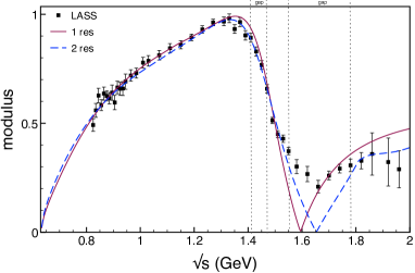
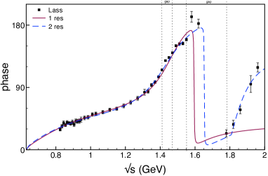
Figure 12: Fits for the modulus and phase of the $K\pi$ $S_{1/2}$ LASS data; points within the regions indicated as gap in the top axis were excluded from the fit.

In Fig.13 we show the real and imaginary components of the amplitude. One notice that values for the real part at threshold are different, namely 24 and 30, and they can be compared with those obtained by ChPTBernard and dispersion relationsMoussalam , respectively T = 21.7 and T = 25.5. These values indicate that the low energy fit is more suitable to describe low energy behaviour.

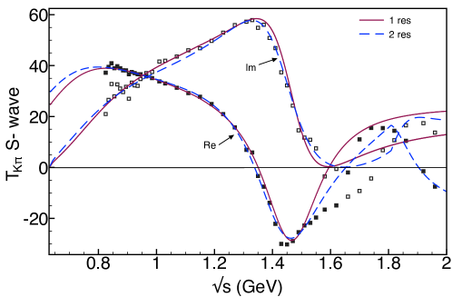
Figure 13: Real and imaginary components of the $S_{1/2}$ $K\pi$ amplitude fitted to LASS data (squares) and extended to low-energies using chiral symmetry.

It is worth noting that both real and imaginary components are very small for $\sqrt{s}\sim 1.65\,$GeV in the two-resonance result.

Appendix D loop integrals

$$I_{abc}^{S} \!=\! \int\frac{d^{4}\ell}{(2\pi)^{4}}\;\frac{16\pi^{2}}{D_{a}\,D_{b}\,D_{c}}\;,\;\;\;I_{abcd}^{S}=\int\frac{d^{4}\ell}{(2\pi)^{4}}\;\frac{16\pi^{2}}{D_{a}\,D_{b}\,D_{c}\,D_{d}}\;.$$

We begin by discussing the integrals $I^{S}$, given by eqs.(7). Their treatment can be simplified because the $\rho$ and the $c\bar{s}$ state entering the form factor share the same momentum. This allows, for instance, one to write

$$I_{\pi K\rho V}^{S} \!=\! \frac{1}{M_{V}^{2}\!-\!\Theta_{R}+i\Theta_{I}}\left[I_{\pi KV}^{S}-I_{\pi K\rho}^{S}\right]\;,$$ (50)

where $\Theta$ is the parameter defined in App.B. Similar simplifications can be performed every time subscripts $\rho V$ or $\rho S$ occur.

The integral $I_{\pi K\rho}^{S}$ is important in this problem because its imaginary part is determined by two different thresholds, associated with cuts along $K\pi$ and $K\rho$ propagators. Using results from App.B, one writes

$$I_{\pi K\rho}^{S} \!=\! \int\frac{d^{4}\ell}{(2\pi)^{4}}\;\frac{16\pi^{2}}{[(\ell\!-\!p_{3})^{2}\!-\!M_{\pi}^{2}]\,[(\ell\!-\!P)^{2}\!-\!M_{K}^{2}]}\;\frac{N_{\rho}}{\ell^{2}-\Theta_{R}+i\Theta_{I}}\;.$$ (51)

Representing this function by means of Feynman parameters and performing one of the integrals analytically, one finds

$$I_{\pi K\rho}^{S} \!=\! i\,N_{\rho}\;\Pi_{\pi K\rho}\;,$$ (52)

$$\Pi_{\pi K\rho} \!=\! -\int_{0}^{1}\!\!da\;J_{\pi K\rho}(a)\;,$$ (53)

with

$$J_{\pi K\rho}(a) \!=\! \frac{1}{\sqrt{\lambda}}\left\{\left[\;\ln\frac{|F_{1}|\,|G_{2}|}{|G_{1}|\,|F_{2}|}\;\right]+i\,\left[\;\theta_{J}\;\right]\right\}\;.$$ (54)

$$\theta_{J} \!=\! \left[\;\theta_{F1}-\theta_{F2}-\theta_{G1}+\theta_{G2}\;\right]\;,$$ (55)

$$F_{1,2} \!=\! \frac{|2M_{D}^{2}\,a+B\mp\sqrt{\lambda}|}{M_{D}^{2}}\;e^{i\,\theta_{F1,2}}\;,$$ (56)

$$G_{1,2} \!=\! \frac{|B\mp\sqrt{\lambda}|}{M_{D}^{2}}\;e^{i\,\theta_{G1,2}}\;,$$ (57)

and

$$B \!=\! \left[\Theta_{R}-i\Theta_{I}-M_{\pi}^{2}-M_{K}^{2}+m_{12}^{2}-a\,(M_{D}^{2}-M_{\pi}^{2}+m_{12}^{2})\right]\;,$$ (58)

$$\lambda \!=\! B^{2}-4\,M_{D}^{2}\,C\;,$$ (59)

$$C \!=\! \left[(1\!-\!a)\,M_{\pi}^{2}+a\,M_{K}^{2}-a\,(1\!-\!a)\,m_{12}^{2}\,\right]\;.$$ (60)

The $\rho$ width is incorporated into the factors $N_{\rho}$, $\Theta_{I}\,$, and the case of a point-like resonance is recovered by making $N_{\rho}\rightarrow 1\,$, $\Theta_{I}\rightarrow\epsilon\,$.

The integral $I_{\pi KV}^{S}$ is

$$I_{\pi KV}^{S} \!=\! \int\frac{d^{4}\ell}{(2\pi)^{4}}\;\frac{16\pi^{2}}{[(\ell\!-\!p_{3})^{2}\!-\!M_{\pi}^{2}]\,[(\ell\!-\!P)^{2}\!-\!M_{K}^{2}]}\;\frac{1}{\ell^{2}-m_{V}^{2}}=i\,\Pi_{\pi KV}\;,$$ (61)

and its evaluation is totally similar. However, as now $m_{V}>M_{D}\,$, its imaginary part comes just from the cut of the diagram along the $K\pi$ subsystem. Integrals $I_{\pi\rho V}^{S}$, $I_{K\rho V}^{S}$ and $I_{K\rho S}^{S}$ do not depend on $m_{12}^{2}$.

References

(1) D. Aston et al., Nucl.Phys. B 296, 493 (1988).
(2) P. Estabrooks et al.,
Nucl. Phys. B 133, 490 (1978).
(3) E.M. Aitala et al.
(E791), Phys. Rev. Lett. 89, 121801 (2002).
(4)
J.M. Link et al. [FOCUS Collaboration],
Phys. Lett. B 681, (2009) 14;
(5) L-L. Chao, Phys. Rep. 95, 1 (1983).
(6) Bauer, Stich and Wirbel, Z. Phys. C 34, 103 (1987)]
(7) Ya. Azimov, J. Phys. G 37, 023001 (2010).
(8) K.S.F.F. Guimarães, W. de Paula, I. Bediaga,
A. Delfino, T. Frederico, A. C. dos Reis
and L. Tomio, Nucl. Phys. B (Proc. Suppl.) 199 (2010) 341.
(9) Z-Y. Zhou, Q-C. Wang and Q. Gao,
Chin. Phys. C 33, XXX (2009).
(10) I. Caprini, Phys. Lett. B 638 468 (2006).
(11) Bochao Liu, M. Buescher, Feng-Kun Guo, C. Hanhart,
and Ulf-G. Meissner, Eur. Phys. J. C 63 93 (2009),
(12) Ulf-G. Meissner and S. Gardner, Eur. Phys. J. A 18
543 (2003).
(13) H. Kamano, S.X. Nakamura, T.-S.H. Lee and T. Sato,
Phys. Rev. D 84, 114019 (2011).
(14) M. Diakonou and F. Diakonos,
Phys. Lett. B 216, 436 (1989)
(15) D. R. Boito, R. Escribano,
Phys. Rev. D 80, 054007 (2009).
(16) P. C. Magalhães, M. R. Robilotta,
K. S. F. F. Guimarães, T. Frederico,W. de Paula,
I. Bediaga, A. C. dos Reis, C.M. Maekawa and G.R.S. Zarnauskas,
Phys. Rev. D84, 094001 (2011).
(17) S. X. Nakamura, arXiv:1504.02557 (2015).
(18) S. Weinberg, Physica A 96, 327 (1979).
(19) J. Gasser and H. Leutwyler,
Nucl. Phys. B250, 465 (1985);
Ann. Phys. 158, 142 (1984).
(20) G. Ecker, J. Gasser, A. Pich and E. De Rafael,
Nucl. Phys. B 321, 311 (1989).
(21) J.A. Oller and E. Oset,
Phys. Rev. D 60, 074023 (1999);
Nucl. Phys. A 620, 465 (1997); A 652, 407(E) (1999).
(22) G. Burdman and J.F. Donoghue,
Phys. Lett. B 280, 287 (1992);
M.B. Wise, Phys.Rev. D45, R2188 (1992).
(23) D.R. Boito and M.R. Robilotta,
Phys. Rev. D 76, 094011 (2007).
(24)
R. Casalbuoni, A. Deandrea, N. Di Bartolomeo, R. Gatto, F. Feruglio
and G. Nardulli, Pys.Rep. 281, 145 (1997).
(25) B. Hyams et. al., Nucl. Phys. B64, 134 (1973).
(26) R. Higa and M.R. Robilotta,
Phys.Rev. C68, 024004 (2001).
(27) P.C. Magalhães, Ph.D. Thesis,
University of São Paulo (2014).
(28) G. Colangelo, J. Gasser and H. Leutwyler,
Nucl. Phys. B 603, 125 (2001).
(29) P.C. Magalhães and M.R. Robilotta, Phys.Rev. D 90, 014043-1 (2014).
(30)
P. Büttiker, S. Descotes-Genon and B. Moussalam,
Eur. J. Phys. C 33, 409 (2004).
(31)
V. Bernard, N. Kaiser and U.G. Meissner, Nucl. Phys. B 357, 129 (1991).