Multisensor CPHD filter

Abstract

The single sensor probability hypothesis density (PHD) and cardinalized probability hypothesis density (CPHD) filters have been developed in the literature using the random finite set framework. The existing multisensor extensions of these filters have limitations such as sensor order dependence, numerical instability or high computational requirements. In this paper we derive update equations for the multisensor CPHD filter. The multisensor PHD filter is derived as a special case. Exact implementation of the multisensor CPHD involves sums over all partitions of the measurements from different sensors and is thus intractable. We propose a computationally tractable approximation which combines a greedy measurement partitioning algorithm with the Gaussian mixture representation of the PHD. Our greedy approximation method allows the user to control the tradeoff between computational overhead and approximation accuracy.

I Introduction

In the multitarget tracking problem often the number of targets and the number of observations detected by sensors are unknown and time varying. Thus representing the targets and observations as vectors is inefficient. A finite set is a more suitable representation. This is the motivation for the random finite set framework [1, 2] which represents target states and observations as realizations of random finite sets. The implementation of the general multitarget Bayes filter for random finite sets is analytically and computationally infeasible [3]. Several approximations have been proposed which make suitable assumptions to derive tractable filters [3, 4, 5, 6, 7].

The majority of research based on random finite set theory has focused on single sensor multitarget tracking. The probability hypothesis density (PHD) filter [3] propagates, over time, the probability hypothesis density function which is defined over the single target state space. Improving on the PHD filter, the cardinalized probability hypothesis density (CPHD) filter [4] propagates the distribution of the number of targets (the cardinality) in addition to the PHD function. Various implementations of the PHD and CPHD filter have been proposed, including the Gaussian mixture implementation [5, 6] and the sequential Monte Carlo implementation [7]. These algorithms have been successfully applied to the problem of multitarget tracking in the presence of clutter.

A general multisensor extension of the PHD filter was first derived for the case of two sensors by Mahler [8, 9]. The filter equations were further generalized to include an arbitrary number of sensors by Delande et al. [10]. Because of their combinatorial nature, the exact filter update equations of the general multisensor PHD filter are not computationally tractable except for a very few simple cases. Delande et al. [11, 12] derive simplifications to the filter update equations for the case when the fields of view of different sensors have limited overlap. This reduces the computational complexity to some extent, and a particle filter based implementation is presented in [12]. Jian et al. [13] suggest implementing the general multisensor PHD filter by repeated application of the two sensor PHD filter [8]. The implementation details for realizing the general multisensor PHD filter in this manner are not made explicit, and the reported numerical simulations are restricted to the case of two sensors.

To avoid the combinatorial computational complexity of the general multisensor PHD filter, some approximate multisensor filters have been proposed in the literature. The iterated-corrector PHD filter [9] processes the information from different sensors in a sequential manner. A single sensor PHD filter processes measurements from the first sensor. Using the output PHD function produced by this step as the predicted PHD function, another single sensor PHD filter processes measurements from the second sensor and so on. As a result, the final output strongly depends on the order in which sensors are processed [14]. This dependence on the sensor order can be mitigated by employing the approximate product multisensor PHD and CPHD filters proposed by Mahler [15]. Although the final results are independent of sensor order, Ouyang and Ji [16] have reported that Monte Carlo implementation of the approximate product multisensor PHD filter is unstable and the problem worsens as the number of sensors increases. We have observed a similar instability in Gaussian mixture model-based implementations. Ouyang and Ji [16] have proposed a heuristic fix to stabilise the Monte Carlo implementation but it is not analytically verified. A comprehensive review of the different multisensor multitarget tracking algorithms based on random finite set theory can be found in [17, Ch. 10].

In this paper we derive the update equations for the general multisensor CPHD filter. The derivation method is similar to that of the general multisensor PHD filter [8, 10] with the additional propagation of the cardinality distribution. The multisensor CPHD filter we derive has combinatorial complexity and an exact implementation is computationally infeasible. To overcome this limitation we propose a two-step greedy approach based on a Gaussian mixture model implementation. Each step can be realized using a trellis structure constructed using the measurements from different sensors or measurement subsets for different Gaussian components. The algorithm is applicable to both the general multisensor CPHD and the general multisensor PHD filters.

Other trellis based algorithms have been developed for target tracking. For single-sensor single-target tracking, the Viterbi algorithm is applied over a trellis of measurements constructed over time in [18]. Each column of the trellis is a measurement scan at a different time step. The Viterbi algorithm is used to find the best path in the trellis corresponding to data associations over time. This approach has been extended to multitarget tracking in [19] for a fixed and known number of targets. The nodes of the trellis correspond to different data association hypotheses and the transition weights are based on measurement likelihoods. The Viterbi algorithm was also applied in [20], in conjunction with energy based transition weights, to identify the $K$-best non-intersecting paths over the measurement trellis when $K$ targets are present.

The form of the update equations in the general multisensor PHD/CPHD filters are similar to the update equations of the single sensor PHD/CPHD filters for extended targets [21, 22]. The similarity is in the sense that for extended targets the update equation requires partitioning of the single sensor measurement set which can be computationally demanding. Granstrom et al. [23] propose a Gaussian mixture model-based implementation of the PHD filter for extended targets with reduced partitioning complexity. This is done by calculating the Mahalanobis distance between the measurements and grouping together measurements which are close to each other within a certain threshold. Orguner et al. [22] use a similar method to reduce computations in the Gaussian mixture model-based implementation of the CPHD filter for extended targets.

The rest of the paper is organized as follows: Section II provides a brief overview of random finite sets. Section III formally poses the problem of multisensor multitarget tracking. In Section IV we summarize the prediction and update equations of the general multisensor CPHD filter. The derivation of the filter update equations is provided in the appendices. We present computationally tractable implementations of the general multisensor PHD and CPHD filters in Section V. A performance comparison of the proposed filter with existing multisensor filters is conducted using numerical simulations in Section VI. We provide conclusions in Section VII.

Portions of this work are presented in a conference paper [24]; the present manuscript contains detailed derivations and proofs which were omitted from the conference paper, and the present manuscript also includes a more detailed description and evaluation of the proposed approximation and implementation of the general multisensor PHD and CPHD filters.

II Background on random finite sets

II-A Random finite sets

Random finite sets are set-valued random variables. The PHD and CPHD filters are derived using notions of random finite sets. This section provides a review of this background, introducing definitions and notation used in the derivations that follow. Detailed treatments of random finite sets and the related statistics in the context of multitarget tracking can be found in [1, 2, 17].

A random finite set is completely specified using its probability density function if it exists. The probability density function of a random finite set modeling the multitarget state is also referred to as the multitarget density function in this paper. Let $Y$ be a realization of a random finite set $\Xi$ with elements from an underlying space ${\cal Y}$, i.e. $Y\subseteq{\cal Y}$. For the random finite set $\Xi$, denote its density function by $f_{\Xi}(Y)$. Let the cardinality distribution of the random finite set $\Xi$ be $p_{\Xi}(n)$

$$p_{\Xi}(n)\mathrel{\overset{\makebox[0.0pt]{\mbox{\tiny def}}}{=}}\textrm{Prob}(|\Xi|=n)\,,\;n=1,2,\dots\,,$$ (1)

where the notation $|\Xi|$ denotes the cardinality of set $\Xi$. The probability generating function (PGF) of the cardinality distribution $p_{\Xi}(n)$ is defined as

$${M}_{\Xi}(t)\mathrel{\overset{\makebox[0.0pt]{\mbox{\tiny def}}}{=}}\sum_{n=0}^{\infty}t^{n}p_{\Xi}(n).$$ (2)

A statistic of the random finite set, which is used by the PHD and CPHD filters, is the probability hypothesis density (PHD) function [2]. For the random finite set $\Xi$ defined over an underlying space ${\cal Y}$, we denote its PHD by $D_{\Xi}({\mathbf{y}})$, ${\mathbf{y}}\in{\cal Y}$. Unlike the probability density function $f_{\Xi}(Y)$ which is defined over the space of finite sets in ${\cal Y}$, the PHD function $D_{\Xi}({\mathbf{y}})$ is defined over the space ${\cal Y}$. Instead of propagating the complete density function, which can be computationally challenging, the PHD and CPHD filters propagate the low dimensional PHD function over time.

II-B IIDC random finite set

An independent and identically distributed cluster (IIDC) random finite set [4] is completely specified by its cardinality distribution and its spatial density function. Let $\Xi$ be an IIDC random finite set with cardinality distribution $p_{\Xi}(n)$ and the spatial density function $\zeta({\mathbf{y}})$. The probability density function $f_{\Xi}(Y)$ and the PHD $D_{\Xi}({\mathbf{y}})$ of the random finite set $\Xi$ are given by the relations

$$f_{\Xi}(Y) =|Y|!\;p_{\Xi}(|Y|)\,\prod_{{\mathbf{y}}\in Y}{\zeta({\mathbf{y}})}$$ (3)

$$D_{\Xi}({\mathbf{y}}) =\zeta({\mathbf{y}})\,\mu$$ (4)

$$\mu =E(|\Xi|)=\sum_{n=0}^{\infty}n\,p_{\Xi}(n).$$ (5)

Samples from an IIDC random finite set can be generated by first sampling a cardinality $m$ from its cardinality distribution $p_{\Xi}(n)$ and then independently sampling $m$ points from its spatial density function $\zeta({\mathbf{y}})$.

The Poisson random finite set is an example of an IIDC random finite set where the cardinality distribution is assumed to be Poisson. The PHD filter [3] models the multitarget state as a realization of a Poisson random finite set and propagates its PHD function over time. The Poisson random finite set assumption can be undesirable because the variance of the Poisson distribution is equal to its mean, which implies that as the number of targets increases, the error in its estimation becomes larger. To overcome this problem the CPHD filter [4] models the multitarget state as a realization of an IIDC random finite set and propagates its PHD function and cardinality distribution over time. The additional cardinality information allows us to more accurately model the multitarget state.

III Problem formulation

We now specify the multisensor multitarget tracking problem. Let ${\mathbf{x}}_{k,i}\in\mathcal{X}$ be the state of the $i^{th}$ target at time $k$. In most of the tracking literature $\mathcal{X}$ is chosen to be the Euclidean space, $\mathcal{X}={\mathbb{R}}^{n_{{\mathbf{x}}}}$, where $n_{{\mathbf{x}}}$ is the dimension of the single target state. If $n_{k}\geq 0$ targets are present at time $k$, the multitarget state can be represented by the finite set $X_{k}=\{{\mathbf{x}}_{k,1},\ldots{\mathbf{x}}_{k,n_{k}}\}$, $X_{k}\subseteq\mathcal{X}$. We assume that each single target state evolves according to the Markovian transition function $f_{k+1|k}({\mathbf{x}}_{k+1,i}|{\mathbf{x}}_{k,i})$. New targets can arrive and existing targets can disappear at each time step. Let the survival probability of an existing target with state ${\mathbf{x}}$ at time $k$ be given by the function $p_{sv,k}({\mathbf{x}})$.

Multiple sensors make observations about the multiple targets present within the monitored region. Assume that there are $s$ sensors, and conditional on the multitarget state, their observations are independent. Measurements ${\mathbf{z}}^{j}$ gathered by sensor $j$ lie in the space $\mathcal{Z}^{j}$, i.e., ${\mathbf{z}}^{j}\in\mathcal{Z}^{j}$. Let $Z^{j}_{k}=\{{\mathbf{z}}^{j}_{1,k},{\mathbf{z}}^{j}_{2,k},\dots,{\mathbf{z}}^{j}_{m_{j,k}}\}$, $Z^{j}_{k}\subseteq\mathcal{Z}^{j}$ be the set of measurements collected by the $j$-th sensor at time step $k$. The measurement set can be empty. We assume that each target generates at most one measurement per sensor at each time instant $k$. Each measurement is either associated with a target or is generated by the clutter process. Define $Z^{1:s}_{k}=Z^{1}_{k}\cup Z^{2}_{k}\cup\dots\cup Z^{s}_{k}$ to be the collection of measurement sets gathered by all sensors at time $k$. The probability of detection of sensor $j$ at time $k$ is given by $p^{j}_{d,k}({\mathbf{x}})$. The function $h_{j,k}({\mathbf{z}}|{\mathbf{x}})$ denotes the probability density (likelihood) that sensor $j$ makes a measurement ${\mathbf{z}}$ given that it detects a target with state ${\mathbf{x}}$. Denote the probability of a missed detection as $q^{j}_{d,k}({\mathbf{x}})=1-p^{j}_{d,k}({\mathbf{x}})$.

The objective of the multitarget tracking problem is to form an estimate $\widehat{X}_{k}$ of the multitarget state at each time step $k$. This estimate is formed using all the measurements up until time $k$ obtained from all the $s$ sensors which is denoted by $Z^{1:s}_{1:k}=\{Z^{1:s}_{1},Z^{1:s}_{2},\dots,Z^{1:s}_{k}\}$. More generally, we would like to estimate the posterior multitarget state distribution $f_{k|k}(X_{k}|Z^{1:s}_{1:k})$.

IV General multisensor CPHD filter

In this section we develop the CPHD filter equations when multiple sensors are present. The derivation method is similar to the approach used to derive the general multisensor PHD filter equations by Mahler [8] and Delande et al. [10]. Since the CPHD filter explicitly accounts for the cardinality distribution of the multitarget state, the filter update equations are more involved. Specifically, the measurement set partitions are more explicitly listed when compared to the PHD filter update equations [8, 10]. The CPHD filter also requires additional propagation of the cardinality distribution.

We make the following modeling assumptions while deriving the multisensor CPHD filter equations
Assumption 1:

1. Target birth at time $k+1$ is modelled using an IIDC random finite set.

2. The predicted multitarget distribution at time $k+1$ is IIDC.

3. The sensor observation processes are independent conditional on the multitarget state $X_{k+1}$, and the sensor clutter processes are IIDC.

Before deriving the filter equations, we introduce some notation. Let $b_{k+1}({\mathbf{x}})$ be the PHD function and let $p_{b,k+1}(n)$ be the cardinality distribution of the birth process at time $k$. For the $j$-th sensor let $c_{k+1,j}({\mathbf{z}})$ be the clutter spatial distribution and let $C_{k+1,j}(t)$ be the PGF of the clutter cardinality distribution at time $k+1$. Let $D_{k+1|k}({\mathbf{x}})$ denote the predicted PHD function and let $r_{k+1|k}({\mathbf{x}})$ denote the normalized predicted PHD function at time $k+1$ (normalized so that it integrates to one). Let the PGF of the predicted cardinality distribution $p_{k+1|k}(n)$ be denoted by ${M}_{k+1|k}(t)$. To keep the expressions and derivation compact we drop the time index and write

$$c_{k+1,j}({\mathbf{z}}) \equiv c_{j}({\mathbf{z}}),\;C_{k+1,j}(t)\equiv C_{j}(t),\;p^{j}_{d,k+1}({\mathbf{x}})\equiv p^{j}_{d}({\mathbf{x}})$$

$${M}_{k+1|k}(t) \equiv{M}(t),\;q^{j}_{d,k+1}({\mathbf{x}})\equiv q^{j}_{d}({\mathbf{x}}),\;p_{sv,k+1}({\mathbf{x}})\equiv p_{sv}({\mathbf{x}})$$

$$h_{j,k+1}({\mathbf{z}}|{\mathbf{x}}) \equiv h_{j}({\mathbf{z}}|{\mathbf{x}}),\;r_{k+1|k}({\mathbf{x}})\equiv r({\mathbf{x}}),\;m_{j,k+1}\equiv m_{j}$$

$$p_{b,k+1}(n) \equiv p_{b}(n)\,,$$ (6)

when the time is clear from the context. Note that abbreviated notation is used only for convenience and the above quantities are in general functions of time. For functions $a({\mathbf{y}})$ and $b({\mathbf{y}})$, the notation $\langle a,b\rangle$ is defined as $\langle a,b\rangle=\int{a({\mathbf{y}})\,b({\mathbf{y}})\,d{\mathbf{y}}}$. In the following subsections we discuss the prediction and update steps of the general multisensor CPHD filter.

IV-A CPHD prediction step

Since sensor information is not required in the prediction step, the prediction step of the CPHD filter for the multisensor case is the same as that for the single sensor case. Denote the posterior probability hypothesis density at time $k$ as $D_{k|k}({\mathbf{x}})$ and the posterior cardinality distribution as $p_{k|k}(n)$. The predicted probability hypothesis density function at time $k+1$ is given by [4, 6]

$$D_{k+1|k}({\mathbf{x}}) =b_{k+1}({\mathbf{x}})+\int\!{p_{sv}({\mathbf{w}})f_{k+1|k}({\mathbf{x}}|{\mathbf{w}})}D_{k|k}({\mathbf{w}})d{\mathbf{w}}\,,$$ (7)

where the integral is over the complete single target state space. The predicted cardinality distribution at time $k+1$ is given by [4, 6]

$$p_{k+1|k}(n)=$$

$$\,\sum_{j=0}^{n}p_{b}(n-j)\sum_{l=j}^{\infty}{{l\choose j}\frac{{\langle D_{k|k},p_{sv}\rangle}^{j}{\langle D_{k|k},1-p_{sv}\rangle}^{l-j}}{{\langle D_{k|k},1\rangle}^{l}}p_{k|k}(l)}\,,$$ (8)

where $n$, $j$ and $l$ are non-negative integers. The normalized predicted PHD function is given by

$$r({\mathbf{x}})\equiv r_{k+1|k}({\mathbf{x}}) =\frac{D_{k+1|k}({\mathbf{x}})}{\mu_{k+1|k}},$$ (9)

$$\text{where }\quad\mu_{k+1|k} =\sum_{n=1}^{\infty}{n\,p_{k+1|k}(n)}.$$ (10)

IV-B CPHD update step

We use the notation ${\lsem}1,s{\rsem}$ to denote the set of integers from $1$ to $s$. Let $W\subseteq Z^{1:s}_{k+1}$ such that for all $j\in{\lsem}1,s{\rsem}$, $|W|_{j}\leq 1$ where $|W|_{j}=|\{{\mathbf{z}}\in W:{\mathbf{z}}\in Z^{j}_{k+1}\}|$. Thus the subset $W$ can have at most one measurement from each sensor. Let $\mathcal{W}$ be the set of all such $W$. For any measurement subset $W$ we can uniquely associate with it a set of pair of indices $T_{W}$ defined as $T_{W}=\{(j,l):{\mathbf{z}}^{j}_{l}\in W\}$. For disjoint subsets $W_{1},W_{2},\dots W_{n}$, let $V=Z^{1:s}_{k+1}\setminus(\cup_{i=1}^{n}{W_{i}})$, so that $W_{1},W_{2},\dots W_{n}$ and $V$ partition $Z^{1:s}_{k+1}$. Think of the set $W_{i}$ as a collection of measurements made by different sensors, all of which are generated by the same target and the set $V$ as the collection of clutter measurements made by all the sensors. Let $P$ be a partition of $Z^{1:s}_{k+1}$, constructed using elements from the set $\mathcal{W}$ and a set $V$, given by

$$P =\{W_{1},W_{2},\dots W_{|P|-1},V\},$$ (11)

such that $$\bigcup_{i=1}^{|P|-1}W_{i}\cup V=Z^{1:s}_{k+1},$$ (12)

$$W_{i}\cap W_{j}=\emptyset,\text{for any }W_{i},W_{j}\in P,i\neq j$$ (13)

$$W_{i}\cap V=\emptyset,\text{for any }W_{i}\in P$$ (14)

where $|P|$ denotes the number of elements in the partition $P$.

The partition $P$ groups the measurements in $Z^{1:s}_{k+1}$ into disjoint subsets where each subset is either generated by a target (the $W$ subsets) or generated by the clutter process (the $V$ subset). Let $|P|_{j}$ be the number of measurements made by sensor $j$ which are generated by the targets. We have:

$$|P|_{j} =\sum_{i=1}^{|P|-1}{|W_{i}|_{j}}.$$ (15)

The number of measurements made by sensor $j$ which are classified as clutter in the partition $P$ is $(m_{j}-|P|_{j})$. Let ${\cal P}$ be the collection of all possible partitions $P$ of $Z^{1:s}_{k+1}$ constructed as above. A recursive expression for constructing the collection ${\cal P}$ is given in Appendix A.

Denote the $v^{th}$-order derivatives of the PGFs of the clutter cardinality distribution and the predicted cardinality distribution as

$$C^{(v)}_{j}(t) =\frac{d^{v}C_{j}}{dt^{v}}(t)\,,\quad{M}^{(v)}(t)=\frac{d^{v}{M}}{dt^{v}}(t).$$ (16)

We use $\gamma$ to denote the probability, under the predictive PHD, that a target is detected by no sensor, and we thus have:

$$\gamma\mathrel{\overset{\makebox[0.0pt]{\mbox{\tiny def}}}{=}}\int\!r({\mathbf{x}})\prod_{j=1}^{s}{q^{j}_{d}({\mathbf{x}})}d{\mathbf{x}}\,.$$ (17)

For concise specification of the update equations, it is useful to combine the terms associated with the PGF of the clutter cardinality distribution for a partition $P$. Let us define the quantity

$$\kappa_{P}\mathrel{\overset{\makebox[0.0pt]{\mbox{\tiny def}}}{=}}\prod_{j=1}^{s}C^{(m_{j}-|P|_{j})}_{j}(0).$$ (18)

For a set $W\in\mathcal{W}$ and the associated index set $T_{W}$ define the quantities

$$d_{W}\mathrel{\overset{\makebox[0.0pt]{\mbox{\tiny def}}}{=}}\frac{\displaystyle\int\!\!r({\mathbf{x}})\left(\prod_{(i,l)\in T_{W}}{\!\!\!\!p_{d}^{i}({\mathbf{x}})\,h_{i}({\mathbf{z}}^{i}_{l}|{\mathbf{x}})}\right)\,\!\!\!\prod_{j:(j,*)\notin T_{W}}{\!\!\!\!\!\!q^{j}_{d}({\mathbf{x}})}d{\mathbf{x}}}{\displaystyle\prod_{(i,l)\in T_{W}}{c_{i}({\mathbf{z}}^{i}_{l})}},$$ (19)

$$\rho_{W}({\mathbf{x}})\mathrel{\overset{\makebox[0.0pt]{\mbox{\tiny def}}}{=}}\frac{\displaystyle\left(\prod_{(i,l)\in T_{W}}{\!\!\!\!p_{d}^{i}({\mathbf{x}})\,h_{i}({\mathbf{z}}^{i}_{l}|{\mathbf{x}})}\right)\,\prod_{j:(j,*)\notin T_{W}}{\!\!\!\!\!\!q^{j}_{d}({\mathbf{x}})}}{\displaystyle\int\!\!r({\mathbf{x}})\left(\prod_{(i,l)\in T_{W}}{\!\!\!\!p_{d}^{i}({\mathbf{x}})\,h_{i}({\mathbf{z}}^{i}_{l}|{\mathbf{x}})}\right)\,\prod_{j:(j,*)\notin T_{W}}{\!\!\!\!\!\!q^{j}_{d}({\mathbf{x}})}d{\mathbf{x}}},$$ (20)

where $(j,*)$ indicates any pair of indices of the form $(j,l)$. The quantity $d_{W}$ can be interpreted as the ratio of the likelihood that the measurement subset $W$ was generated by the target process to the likelihood that the measurement subset $W$ was generated by the clutter process. The quantity $\rho_{W}({\mathbf{x}})$ can be interpreted as the normalized pseudolikelihood contribution of the measurement subset $W$.

The updated probability hypothesis density function $D_{k+1|k+1}({\mathbf{x}})$ can be expressed as the product of the normalized predicted probability hypothesis density $r_{k+1|k}({\mathbf{x}})$ at time $k+1$ and a pseudolikelihood function. The pseudolikelihood function can be expressed as a linear combination of functions (one function for each partition $P$) with associated weights $\alpha_{P}$. The all-clutter partition $P=\{V\}$ where $V=Z^{1:s}_{k+1}$ has an associated weight $\alpha_{0}$. Define

$$\alpha_{0} \mathrel{\overset{\makebox[0.0pt]{\mbox{\tiny def}}}{=}}\frac{\displaystyle\sum_{P\in{\cal P}}\left(\kappa_{P}{M}^{(|P|)}(\gamma)\prod_{W\in P}{d_{W}}\right)}{\displaystyle\sum_{P\in{\cal P}}\left(\kappa_{P}{M}^{(|P|-1)}(\gamma)\prod_{W\in P}{d_{W}}\right)}\,,$$ (21)

$$\alpha_{P} \mathrel{\overset{\makebox[0.0pt]{\mbox{\tiny def}}}{=}}\frac{\displaystyle\kappa_{P}{M}^{(|P|-1)}(\gamma)\prod_{W\in P}{d_{W}}}{\displaystyle\sum_{Q\in{\cal P}}\left(\kappa_{Q}{M}^{(|Q|-1)}(\gamma)\prod_{W\in Q}{d_{W}}\right)}\,.$$ (22)

Note that the expression $W\in P$ only includes $W\in\mathcal{W}$ and does not include the component $V\in\mathcal{V}$ of $P$. For the all clutter partition $P=\{V\}$ there are no elements in the partition of the type $W$ and we use the convention $\prod_{W\in P}()=1$ whenever $P=\{V\}$. Similary we use the convention $\sum_{W\in P}()=0$ whenever $P=\{V\}$.

Theorem 1.

Under the conditions of Assumption 1, the general multisensor CPHD filter update equation for the probability hypothesis density is

$$\frac{D_{k+1|k+1}({\mathbf{x}})}{r_{k+1|k}({\mathbf{x}})} =\alpha_{0}\,\prod_{j=1}^{s}{q^{j}_{d}({\mathbf{x}})}+\sum_{P\in{\cal P}}\alpha_{P}\,\left(\sum_{W\in P}\rho_{W}({\mathbf{x}})\right)\,$$ (23)

and the update equation for the posterior cardinality distribution is

$$\frac{p_{k+1|k+1}(n)}{p_{k+1|k}(n)} =\frac{\displaystyle\sum_{\begin{subarray}{c}P\in{\cal P}\\ |P|\leq n+1\end{subarray}}\left(\kappa_{P}\frac{n!}{(n-|P|+1)!}\gamma^{n-|P|+1}\prod_{W\in P}{d_{W}}\right)}{\displaystyle\sum_{P\in{\cal P}}\left(\kappa_{P}{M}^{(|P|-1)}(\gamma)\prod_{W\in P}{d_{W}}\right)}\,,$$ (24)

where the quantities $\alpha_{0}$, $\alpha_{P}$, $\rho_{W}({\mathbf{x}})$ and $d_{W}$ are given in (21), (22), (20) and (19), respectively.

The proof of Theorem 1 is provided in Appendix F. It requires the concepts of functional derivatives, probability generating functionals and the multitarget Bayes filter which are revised in Appendices B, C and D respectively. The proof depends on an intermediate result, Lemma 1, which is proved in Appendix E.

IV-C General multisensor PHD filter as a special case

In this section we show that the general multisensor PHD filter can be obtained as a special case of the general multisensor CPHD filter when the following assumptions are made.
Assumption 2:

1. Target birth at time $k+1$ is modelled using a Poisson random finite set.

2. The predicted multitarget distribution at time $k+1$ is Poisson.

3. The sensor observation processes are independent conditional on the multitarget state $X_{k+1}$, and the sensor clutter processes are Poisson.

Since the multitarget state distribution is modelled as Poisson it suffices to propagate the PHD function over time. Let the rate of the Poisson clutter process be $\lambda_{j}$ and let $c_{j}({\mathbf{z}})$ be the clutter spatial distribution for the $j^{th}$ sensor. Let $\mu_{k+1|k}$ be the mean predicted cardinality at time $k+1$. Using the Poisson assumptions for the predicted multitarget distribution and the sensor clutter processes we have

$${M}^{(v)}(\gamma) =\mu_{k+1|k}^{v}\;e^{\mu_{k+1|k}(\gamma-1)}$$ (25)

$$C^{(v)}_{j}(0) =\lambda_{j}^{v}\;e^{-\lambda_{j}}.$$ (26)

Using these in (21) we have the simplification $\alpha_{0}=\mu_{k+1|k}$. We can also simplify the term $\kappa_{P}{M}^{(|P|-1)}(\gamma)$ as

$$\kappa_{P} {M}^{(|P|-1)}(\gamma)=\left(\prod_{j=1}^{s}C^{(m_{j}-|P|_{j})}_{j}(0)\right)\,{M}^{(|P|-1)}(\gamma)$$ (27)

$$=\left(\prod_{j=1}^{s}\lambda_{j}^{m_{j}-|P|_{j}}\,e^{-\lambda_{j}}\right)\,\mu_{k+1|k}^{|P|-1}\;e^{\mu_{k+1|k}(\gamma-1)}$$ (28)

$$=(e^{\mu_{k+1|k}(\gamma-1)-\sum_{j=1}^{s}\lambda_{j}})\left(\prod_{j=1}^{s}\lambda_{j}^{m_{j}}\right)\frac{\mu_{k+1|k}^{|P|-1}}{\left(\prod_{j=1}^{s}\lambda_{j}^{|P|_{j}}\right)}.$$ (29)

Since the expression $\kappa_{P}{M}^{(|P|-1)}(\gamma)$ appears in both the numerator and the denominator of the term $\alpha_{P}$ in the PHD update expression, we can ignore the portion that is independent of $P$. Hence we have

$$\kappa_{P}{M}^{(|P|-1)}(\gamma) \propto\mu_{k+1|k}^{|P|-1}\displaystyle\prod_{j=1}^{s}\lambda_{j}^{-|P|_{j}}.$$ (30)

From (19) and (30), we can write

$$\kappa_{P}{M}^{(|P|-1)}(\gamma)\prod_{W\in P}{d_{W}} \propto\prod_{W\in P}{\tilde{d}_{W}}$$ (31)

where $\tilde{d}_{W}$ is defined as

$$\tilde{d}_{W}\mathrel{\overset{\makebox[0.0pt]{\mbox{\tiny def}}}{=}}$$

$$\frac{\displaystyle\mu_{k+1|k}\int\!\!r({\mathbf{x}})\left(\prod_{(i,l)\in T_{W}}{\!\!\!\!p_{d}^{i}({\mathbf{x}})\,h_{i}({\mathbf{z}}^{i}_{l}|{\mathbf{x}})}\right)\,\prod_{j:(j,*)\notin T_{W}}{\!\!\!\!\!\!q^{j}_{d}({\mathbf{x}})}d{\mathbf{x}}}{\displaystyle\prod_{(i,l)\in T_{W}}{\lambda_{i}\,c_{i}({\mathbf{z}}^{i}_{l})}}\cdot$$ (32)

The PHD update equation then reduces to

$$\frac{D_{k+1|k+1}({\mathbf{x}})}{r_{k+1|k}({\mathbf{x}})}=$$

$$\qquad\mu_{k+1|k}\,\prod_{j=1}^{s}{q^{j}_{d}({\mathbf{x}})}+\sum_{P\in{\cal P}}\frac{\displaystyle\left(\prod_{W\in P}{\tilde{d}_{W}}\right)\,\displaystyle\sum_{W\in P}\rho_{W}({\mathbf{x}})}{\displaystyle\sum_{P\in{\cal P}}\left(\prod_{W\in P}{\tilde{d}_{W}}\right)}\cdot$$ (33)

The above equation is equivalent to the general multisensor PHD update equation given in [8, 10].

V Implementations of the general multisensor CPHD and PHD filters

In the previous section we derived update equations for the general multisensor CPHD filter which propagate the PHD function and cardinality distribution over time. Analytic propagation of these quantities is difficult in general without imposing further conditions. In the next subsection we develop a Gaussian mixture-based implementation of the filter update equations. Although the Gaussian mixture implementation is analytically tractable, it is computationally intractable. In Section V-B and V-C we propose greedy algorithms to drastically reduce computations and develop computationally tractable approximate implementations for the general multisensor CPHD and PHD filters.

V-A Gaussian mixture implementation

We make the following assumptions to obtain closed form updates for equations (23) and (24)
Assumption 3:

1. The probability of detection for each sensor is constant throughout the single target state space; i.e., $p^{j}_{d}({\mathbf{x}})=p^{j}_{d}$, for all ${\mathbf{x}}$.

2. The predicted PHD is a mixture of weighted Gaussian densities.

3. The single sensor observations are linear functions of a single target state corrupted by zero-mean Gaussian noise.

4. The predicted cardinality distribution has finite support; i.e., there exists a positive integer $n_{0}<\infty$ such that $p_{k+1|k}(n)=0$, for all $n>n_{0}$.

From the above assumptions we can express the normalized predicted PHD as a Gaussian mixture model

$$r({\mathbf{x}}) =\sum_{i=1}^{J_{k+1|k}}{w_{k+1|k}^{(i)}\,{\cal N}_{(i)}({\mathbf{x}})}$$ (34)

where $w_{k+1|k}^{(i)}$ are non-negative weights satisfying $\sum_{i=1}^{J_{k+1|k}}{w_{k+1|k}^{(i)}}=1$; and ${\cal N}_{(i)}({\mathbf{x}})\mathrel{\overset{\makebox[0.0pt]{\mbox{\tiny def}}}{=}}{\cal N}({\mathbf{x}};m_{k+1|k}^{(i)},\Sigma_{k+1|k}^{(i)})$ is the Gaussian density function with mean $m_{k+1|k}^{(i)}$ and covariance matrix $\Sigma_{k+1|k}^{(i)}$. If $H_{j}$ is the observation matrix for sensor $j$ then its likelihood function can be expressed as $h_{j}({\mathbf{z}}|{\mathbf{x}})={\cal N}({\mathbf{z}};H_{j}{\mathbf{x}},\Sigma_{j})$. Then under the conditions of Assumption 3, the posterior PHD at time $k+1$ can be expressed as a weighted mixture of Gaussian densities and the posterior cardinality distribution has a finite support.

Since the probability of detection is constant we have $\gamma=\prod_{j=1}^{s}{q^{j}_{d}}$. For each partition $P$ the quantities ${M}^{(|P|-1)}$ and ${M}^{(|P|)}$ can be easily calculated since the predicted cardinality distribution has finite support. The integration in the numerator of (19) is analytically solvable under Assumption 3 and using properties of Gaussian density functions [5]. Hence $d_{W}$ can be analytically evaluated. From these quantities we can calculate $\alpha_{0}$ and $\alpha_{P}$ from (21) and (22). For each measurement set $W$ we can express the product $r({\mathbf{x}})\rho_{W}({\mathbf{x}})$ as a sum of weighted Gaussian densities using the properties of Gaussian density functions [5]. Thus from the update equation (23) the posterior PHD can be expressed as a mixture of Gaussian densities. Since the predicted cardinality distribution has finite support, from (24), the posterior cardinality distribution also has finite support. Similarly, under appropriate linear Gaussian assumptions, the posterior PHD in (33) can be expressed as a mixture of Gaussian densities.

The conditions of Assumption 3 allow us to analytically propagate the PHD and cardinality distribution but the propagation is still numerically infeasible. The combinatorial nature of the update step can be seen from (23), (24) and (33). Specifically, the exact implementation of the general multisensor CPHD and PHD filters would require evaluation of all the permissible partitions (i.e. all $P\in{\cal P}$) that could be constructed from all possible measurement subsets. The number of such partitions is prohibitively large and a direct implementation is infeasible. We now discuss an approximation of the update step to overcome this limitation.

The key idea of the approximate implementation is to identify elements of the collection ${\cal P}$ which make a significant contribution to the update expressions. We propose the following two-step greedy approximation to achieve this within the Gaussian mixture framework. The first approximation step is to select a few measurement subsets $W$ for each Gaussian component. These subsets are identified by evaluating a score function which quantifies the likelihood that the subset was generated by that Gaussian component. The second approximation step is to greedily construct partitions of these subsets which are significant for the update step. The following subsections explain these two steps in detail.

V-B Selecting the best measurement subsets

A measurement subset is any subset of the measurement set $Z^{1:s}_{k+1}$ such that it contains at most one measurement per sensor. The total number of measurement subsets that can be constructed when the $j^{th}$ sensor records $m_{j}$ measurements is $\displaystyle\prod_{j=1}^{s}{(m_{j}+1)}$. When there are many targets present and/or the clutter rate is high this number can be very large. Since the size of the collection ${\cal P}$ depends on the number of measurement subsets, to develop a tractable implementation of the update step it is necessary to limit the number of measurement subsets. Instead of enumerating all possible measurement subsets, they are greedily and sequentially constructed and only a few are retained based on the scores associated with them.

Consider the measurement subset $W$ and the associated set $T_{W}$ as defined earlier. For the $i^{th}$ Gaussian component and the measurement subset $W$ we can associate a score function $\beta^{(i)}(W)$ defined as

$$\beta^{(i)}(W) \mathrel{\overset{\makebox[0.0pt]{\mbox{\tiny def}}}{=}}\frac{\displaystyle\int\!\!{\cal N}_{(i)}({\mathbf{x}})\left(\prod_{(j,l)\in T_{W}}{\!\!\!\!p_{d}^{j}\,h_{j}({\mathbf{z}}^{j}_{l}|{\mathbf{x}})}\right)\left(\prod_{j:(j,*)\notin T_{W}}{\!\!\!\!\!\!q^{j}_{d}}\right)d{\mathbf{x}}}{\displaystyle\prod_{(j,l)\in T_{W}}{c_{j}({\mathbf{z}}^{j}_{l})}}\cdot$$ (35)

The above score function is obtained by splitting the $d_{W}$ term in (19) for each Gaussian component. Intuitively, this score can be interpreted as the ratio of the likelihood that the measurement subset $W$ was generated by the single target represented by the $i^{th}$ Gaussian component to the likelihood that the measurement subset $W$ was generated by the clutter process. The score $\beta^{(i)}(W)$ can be analytically calculated since the integral is solvable under Assumption 3 and using properties of Gaussian densities [7]. The score is high when the elements of the set $W$ truly are the measurements caused by the target associated with the $i^{th}$ Gaussian component. We use $\beta^{(i)}(W)$ to rank measurement subsets for each Gaussian component and retain only a fraction of them with the highest scores.

Figure 1: Trellis diagram for constructing measurement subsets for each Gaussian component. Solid blue lines represent measurement subsets retained after processing sensors 1 to 3. Dashed red lines correspond to extensions of retained measurement subsets when processing measurements from sensor $4$.

For each Gaussian component, we select the measurement subsets by randomly ordering the sensors and incrementally incorporating information from each sensor in turn. We retain a maximum of $W_{\textrm{max}}$ subsets at each step. Figure 1 provides a graphical representation of the algorithm in the form of a trellis diagram. Each column of the trellis corresponds to observations from one of the sensors. The sensor number is indicated at the top of each column. The nodes of the trellis correspond to the sensor observations $({\mathbf{z}}_{1}^{1},{\mathbf{z}}_{2}^{1},\dots,\,{\mathbf{z}}_{1}^{2},{\mathbf{z}}_{2}^{2},\dots)$ or the no detection case $({\mathbf{z}}_{\emptyset}^{1},{\mathbf{z}}_{\emptyset}^{2},\dots)$.

The process of sequential construction of measurement subsets can be demonstrated using an example as follows. The solid lines in Figure 1 represent partial measurement subsets retained after processing observations from sensors 1 to 3. Now consider the measurement subset indicated by the thick solid line. It corresponds to the measurement subset $\{{\mathbf{z}}_{1}^{2},{\mathbf{z}}_{1}^{3}\}$. When the sensor $4$ measurements are processed, this measurement subset is extended for each node of sensor $4$ as represented by the dashed lines. The scores $\beta^{(i)}(W)$ are calculated for these new measurement subsets using the expression in (35) but limited to only the first $4$ sensors. This is done for each existing measurement subset in the sensor-measurement space and $W_{\textrm{max}}$ measurement subsets with highest scores are retained and considered at the next sensor. Although the process of constructing measurement subsets is dependent on the order in which sensors are processed, we observe from simulations that it has no significant effect on filter performance. Once the subsets have been selected, the ordering has no further effect in the update process.

V-C Constructing partitions

The algorithm to construct partitions from subsets is similar to the above algorithm used to identify the best measurement subsets. Since the $V$ component of a partition is unique given the $W$ components, it is sufficient to identify the $W$ components to uniquely specify a partition $P$. A graphical representation of the algorithm is provided in Figure 2. Each column of this trellis corresponds to the set of measurement subsets $\{W^{i}_{1},W^{i}_{2},\dots\}$ identified by the $i^{th}$ Gaussian component. The component number $(i)$ is indicated at the top of each column. The node $W_{\emptyset}^{i}$ represents the empty measurement subset $W_{\emptyset}^{i}=\emptyset$ which is always included for each component and it corresponds to the event that the Gaussian component was not detected by any of the sensors. With each valid partition $P$ we associate the score $d_{P}=\displaystyle\prod_{W\in P}{d_{W}}$ with $d_{\emptyset}=1$.

Figure 2: Trellis diagram for constructing partitions. Solid blue lines represent partitions retained after processing Gaussian components 1 to 3. Red dashed lines correspond to partition extension when incorporating measurement subsets corresponding to the $4^{th}$ Gaussian component.

We greedily identify partitions of subsets by incrementally incorporating measurement subsets from the different components. For example the solid lines in Figure 2 correspond to the partitions that have been retained after processing components number 1 to 3. The existing partitions are expanded using the measurement subsets from the $4^{th}$ component as indicated by the dashed lines. Some extensions are not included as they do not lead to a valid partition. Since the empty measurement subset $W_{\emptyset}^{i}$ is always included in the trellis, a partition can always be found. We process the Gaussian components in decreasing order of their associated weights. After processing each component, we retain a maximum of $P_{\textrm{max}}$ partitions corresponding to the ones with highest $d_{P}$. These selected partitions of measurement subsets are used in the update equations (23), (24) and (33) to compute the posterior PHDs and cardinality distribution. In our current implementation we select measurement subsets and construct measurement partitions using only the prior PHD information. Future research can focus on enhancing this construction procedure by including the current measurements along with the prior PHD.

For the general multisensor PHD filter a slightly more accurate implementation can be used and is described as follows. After the first approximate step of identifying measurement subsets for each Gaussian component, instead of the approximate partition construction discussed in this section, we can find all possible partitions from the given collection of measurement subsets. This problem of finding all partitions can be mapped to the exact cover problem [25]. An efficient algorithm called Dancing Links has been suggested by Knuth [26] for solving this problem. This implementation can be used when the number of sensors and measurement subsets are small.

VI Numerical simulations

In this section we compare different multisensor multitarget tracking algorithms developed using the random finite set theory. Specifically we compare the following filters: iterated-corrector PHD (IC-PHD [8]), iterated-corrector CPHD (IC-CPHD), general multisensor PHD (G-PHD) and the general multisensor CPHD (G-CPHD) filter derived in this paper. Models used to simulate multitarget motion and multisensor observations are discussed in detail in the next subsections. The simulated observations are used by different algorithms to perform multitarget tracking. All the simulations were conducted using MATLAB .

VI-A Target dynamics

The single target state is a four dimensional vector ${\mathbf{x}}=[x,y,v_{x},v_{y}]$ consisting of its position coordinates $x$ and $y$ and its velocities $v_{x}$ and $v_{y}$ along the $x$-axis and $y$-axis respectively. The target state evolves according to the discretized version of the continuous time nearly constant velocity model [27] given by

$${\mathbf{x}}_{k+1,i} =\left[\begin{array}[]{cccc}1&0&T&0\\ 0&1&0&T\\ 0&0&1&0\\ 0&0&0&1\end{array}\right]{\mathbf{x}}_{k,i}+\eta_{k+1,i}$$ (40)

$$\eta_{k+1,i} \sim{\cal N}({\bf 0},\Sigma_{\eta})\,,\;\Sigma_{\eta}=\left[\begin{array}[]{cccc}\frac{T^{3}}{3}&0&\frac{T^{2}}{2}&0\\ 0&\frac{T^{3}}{3}&0&\frac{T^{2}}{2}\\ \frac{T^{2}}{2}&0&T&0\\ 0&\frac{T^{2}}{2}&0&T\end{array}\right]\sigma_{\eta}^{2}$$ (45)

where $T$ is the sampling period and $\sigma_{\eta}^{2}$ is the intensity of the process noise. We simulate $100$ time steps with a sampling period of $T=1s$ and process noise intensity of $\sigma_{\eta}=0.25m$. Figure 3(a) shows the target tracks used in the simulations and Figure 3(b) shows the variation of the number of targets over time. All the targets originate from one of the following four locations $(\pm 400m,\pm 400m)$ and targets are restricted to the $2000m\times 2000m$ square region centered at the origin. Targets 1 & 2 are present in the time range $k\in{\lsem}1,100{\rsem}$; targets 3 & 4 for $k\in{\lsem}21,100{\rsem}$; targets 5 & 6 for $k\in{\lsem}41,100{\rsem}$; and targets 7 & 8 for $k\in{\lsem}61,80{\rsem}$.

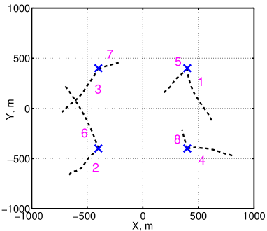
(a) Target tracks

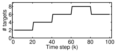
(b) Cardinality

Figure 3: (a): Evolution of target tracks. The blue cross indicates origin of target trajectory. (b): Number of targets as function of time.

VI-B Measurement model

Measurements are collected independently by six sensors. When a sensor detects a target, the corresponding measurement consists of the position coordinates of the target corrupted by additive Gaussian noise. Thus if a target located at $(x,y)$ is detected by a sensor, the measurement gathered by the sensor is given by

$${\mathbf{z}}=\left[\begin{array}[]{c}x\\ y\end{array}\right]+\left[\begin{array}[]{c}w_{x}\\ w_{y}\end{array}\right]$$ (50)

where $w_{x}$ and $w_{y}$ are independent zero-mean Gaussian noise terms with standard deviation $\sigma_{w_{x}}$ and $\sigma_{w_{y}}$ respectively. In our simulations we use $\sigma_{w_{x}}=\sigma_{w_{y}}=10m$. The probability of detection of each sensor is constant throughout the monitoring region. Five of the sensors have a fixed probability of detection of $0.5$. The probability of detection of the sixth sensor is variable and is changed from $0.2$ to $1$ in increments of $0.1$. The clutter measurements made by each of the sensors is Poisson with uniform spatial density and mean clutter rate $\lambda=10$.

VI-C Filter implementation details and error metric

All the filters model the survival probability at all times and at all locations as constant with $p_{sv}=0.99$. The target birth intensity is modelled as a Gaussian mixture with four components centered at $(\pm 400,\pm 400,0,0)$, each with covariance matrix diag$([100,100,25,25])$ and weight $0.1$. The target birth cardinality distribution is assumed Poisson with mean $0.4$. We consider two cases of sensor ordering where the sensor with variable probability of detection is either processed first (Case 1) or last (Case 2).

For the different multisensor filters the PHD function is represented by a mixture of Gaussian densities whereas the cardinality distribution is represented by a vector of finite length which sums to one. This Gaussian mixture model approximation was first used in [5] and [6] for multitarget tracking using single sensor PHD and CPHD filters respectively. We perform pruning of Gaussian components with low weights and merging of Gaussian components in close vicinity [5] for computational tractability. For the iterated-corrector filters pruning and merging is done after processing each sensor since many components have negligible weight and propagating them has no significant impact on tracking accuracy. For the general multisensor PHD and CPHD filters pruning and merging is performed at the end of the update step since intermediate Gaussian components are not accessible. The general multisensor PHD and CPHD filters are implemented using the two-step greedy approach described in Section V. In our simulations the maximum number of measurement subsets per Gaussian component is set to $W_{\textrm{max}}=6$ and the maximum number of partitions of measurement subsets is set as $P_{\textrm{max}}=6$. For CPHD filters, the cardinality distribution is assumed to be zero for $n>20$.

For the PHD filters, we estimate the number of targets by rounding the sum of weights of the Gaussian components to the nearest integer. For the CPHD filters, we estimate the number of targets as the peak of the posterior cardinality distribution. For all the filters, the target state estimates are the centres of the Gaussian components with highest weights in the posterior PHD. To reduce the computational overhead, after each time step we restrict the number of Gaussian components to a maximum of four times the estimated number of targets. When the estimated number of targets is zero we retain a maximum of four Gaussian components.

The tracking performance of the different filters are compared using the optimal sub-pattern assignment (OSPA) error metric [28]. For the OSPA metric, we set the cardinality penalty factor $c=100$ and power $p=1$. The OSPA error metric accounts for error in estimation of target states as well as the error in estimation of number of targets. Given the two sets of estimated multitarget state and the true multitarget state, it finds the best permutation of the larger set which minimizes its distance from the smaller set and assigns a fixed penalty $c$ for each cardinality error. We use the Euclidean distance metric and consider only the target positions while computing the OSPA error.

VI-D Results

The target tracks shown in Figure 3(a) are used in all the simulations. The generated observation sequence is changed by providing a different initialization seed to the random number generator. We generate 100 different observation sequences and report the average OSPA error obtained by running each multisensor filter over these 100 observation sequences. The probability of detection of the sensor with variable probability of detection is gradually increased from $0.2$ to $1$. Figure 4(a) shows the average OSPA error as the probability of detection is changed for the two cases, Case 1 and Case 2. The IC-PHD filter performs significantly worse than all the other filters. For the IC-PHD filter Case 1, the accuracy improves relative to Case 2 as the probability of detection is increased since the sensor with more reliable information is processed towards the end.

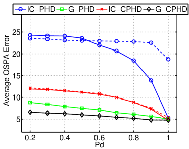
(a) Solid lines: Case 1; Dashed lines: Case 2

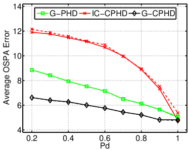
(b) Solid lines: Case 1; Dashed lines: Case 2

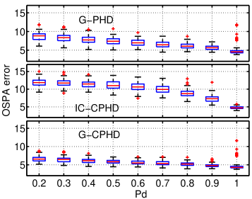
(c) Box and whisker plot

Figure 4: (a): Average OSPA error versus the probability of detection $p_{d}$ of the variable sensor. The solid and dashed lines correspond to Case 1 and Case 2, respectively. (b): A zoomed-in version of the figure in (a) focusing on the IC-CPHD, G-PHD and G-CPHD filters. (c): Box and whisker plot of the OSPA error as a function of $p_{d}$. Boxes indicate 25-75 interquartile range; whiskers extend 1.5 times the range and ‘+’ symbols indicate outliers lying beyond the whiskers.

Figure 4(b) shows a portion of Figure 4(a) enlarged for clarity. We observe that for the G-PHD, IC-CPHD and G-CPHD filters there is very little difference between performance for Case 1 and Case 2. Thus the IC-CPHD filter performance does not depend significantly on the order in which sensors are processed. For the G-PHD and G-CPHD filters the order in which sensors are processed to greedily construct measurement subsets has little impact on the final filter performance. The G-CPHD filter is able to outperform both the G-PHD and the IC-CPHD filters and has the lowest average OSPA error. A box and whisker plot comparison of the G-PHD, IC-CPHD and G-CPHD filters is shown in Figure 4(c). The median OSPA error and the $25-75$ percentiles are shown for different values of $p_{d}$ for the sensor with variable probability of detection.

We now examine the effect of the parameters $W_{\text{max}}$ and $P_{\text{max}}$, i.e., the maximum number of measurement subsets and the maximum number of partitions. $W_{\text{max}}$ is varied in the range $\{1,2,4,6,8,10\}$ and $P_{\text{max}}$ is varied in the range $\{1,2,4,6,8,10\}$. For this simulation we fix the probability of detection of all the six sensors to be $0.5$. All other parameters of the simulation are the same as before. We do tracking using the same tracks as before and over 100 different observation sequences for each pair of $(W_{\text{max}},P_{\text{max}})$.

Figure 5(a) plots the effect of changing $W_{\text{max}}$ and $P_{\text{max}}$ on the average OSPA error and the average computational time required per time-step. Simulations were performed using algorithms implemented in Matlab on computers with two Xeon 4-core 2.5GHz processors and 14GB RAM. Each curve is obtained by fixing $P_{\text{max}}$ and changing $W_{\text{max}}$. Dashed curves correspond to G-PHD filter and solid curves correspond to G-CPHD filters. For a given pair of $(W_{\text{max}},P_{\text{max}})$ values both the filters require almost the same computational time but the G-CPHD filter has a lower average OSPA error compared to the G-PHD filter. We observe that for each curve as $W_{\text{max}}$ increases the average OSPA error reaches a minimum quickly (around $W_{\text{max}}=2$) and then starts rising. This is because as $W_{\text{max}}$ is increased the non-ideal measurement subsets also get involved in the construction of partitions leading to noise terms in the update. The computational time required grows approximately linearly with increase in $W_{\text{max}}$. As $P_{\text{max}}$ is varied the average OSPA error saturates at around $P_{\text{max}}=4$ and increasing it beyond 4 has very little impact. Increasing $P_{\text{max}}$ does not significantly raise the computational time requirements of the approximate G-PHD and G-CPHD filter implementations.

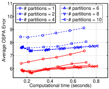
(a) Solid lines: G-CPHD; Dashed lines: G-PHD

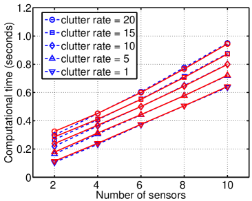
(b) Solid lines: G-CPHD; Dashed lines: G-PHD

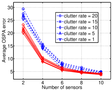
(c) Solid lines: G-CPHD; Dashed lines: G-PHD

Figure 5: (a): Average OSPA error versus computational time per time-step obtained by changing $W_{\text{max}}$ in the range $\{1,2,4,6,8,10\}$ and $P_{\text{max}}$ in the range $\{1,2,4,6,8,10\}$. Blue dashed curves correspond to G-PHD filter and red solid curves correspond to G-CPHD filter. (b): Computation time required as a function of number of sensors. (c): Average OSPA error as a function of number of sensors.

We perform another set of simulations to study the effect of the number of sensors and clutter rate of the sensors on filter performance. In this simulation the number of sensors $s$ is varied in the range $\{2,4,6,8,10\}$ and the clutter rate $\lambda$ of the Poisson clutter process is varied in the range $\{1,5,10,15,20\}$ and is same for all the sensors. We fix the probability of detection of all the sensors to be $0.5$. The approximate greedy algorithm parameters are set to $W_{\text{max}}=6$ and $P_{\text{max}}=6$. All other parameters of the simulation are unchanged. Tracking is performed using the same target tracks as before and 100 different observation sequences are generated for each pair of $(s,\lambda)$.

Figures 5(b) and 5(c) plot the average computational time and the average OSPA error as the number of sensors is changed for different clutter rate values. Each curve is obtained by fixing the clutter rate and changing the number of sensors. Dashed curves correspond to the G-PHD filter and solid curves correspond to the G-CPHD filters. From Figure 5(b) we observe that for approximate greedy implementations of the G-PHD and G-CPHD filters the computational requirements grow linearly with the number of sensors. As the number of sensors is increased the average OSPA error reduces as seen from Figure 5(c). The G-CPHD filter requires relatively fewer sensors to achieve the same accuracy as that of the G-PHD filter.

VI-E Extension to non-linear measurement model

In this section we extend the Gaussian mixture based filter implementation discussed in Section V to include non-linear measurement models using the unscented Kalman filter [29] approach. The unscented extensions to non-linear models when a single sensor is present are discussed in [5] and [6] for the PHD and CPHD filters respectively. We implement the unscented versions of the general multisensor PHD and CPHD filters by repeatedly applying the equations provided in [5, 6]. Specifically, the equations are recursively applied for each ${\mathbf{z}}\in W$ to evaluate the score function $\beta^{(i)}(W)$ while constructing the measurement subsets.

As an example, we consider the setup described in [30] based on at-sea experiments. Two targets are present within the monitoring region and portions of their tracks are shown in Figure 6(b). The target state ${\mathbf{x}}=[x,y]$ consists of its coordinates in the $x-y$ plane and the filters model the motion of individual targets using a random walk model given by ${\mathbf{x}}_{k+1,i}={\mathbf{x}}_{k,i}+\eta_{k+1,i}$ where the process noise $\eta_{k+1,i}$ is zero-mean Gaussian with covariance matrix $\Sigma_{\eta}=\sigma_{\eta}^{2}\,\text{diag}(1,1)$. In our simulations we set $\sigma_{\eta}=0.24\,\text{km}$. Although we consider linear target dynamics in this paper, the unscented approach can be easily extended to include non-linear target dynamics as well.

The targets are monitored using acoustic sensors which collect bearings (angle) measurements. If sensor $j$ is present at location $[x^{j},y^{j}]$ and a target detected by the sensor has coordinates $[x,y]$ then the measurement made by this sensor is given by

$$z =\text{arctan}\left(\frac{y-y^{j}}{x-x^{j}}\right)+w$$ (51)

where the measurement noise $w$ is zero mean Gaussian with standard deviation $\sigma_{w}$ and ‘arctan’ denotes the four-quadrant inverse tangent function. The sensor locations are assumed to be known. The measurements $z$ are in the range $[0,360)$ degrees. Along with the target related measurements the sensors also record clutter measurements not associated with any target. Five sensors (which slowly drift over time) gather measurements and their approximate locations are indicated in Figure 6(b). To demonstrate the feasibility of the proposed algorithms for non-linear measurement models, in this paper we consider sensor deployments and target trajectories based on at-sea experiments. The sensor measurements themselves are simulated to avoid the issue of measurement model mismatch. All sensors are assumed to have the same $\sigma_{w}$ and we vary $\sigma_{w}$ in the range $\{1,2,3,4\}$ (degrees) in our simulations. The probability of detection of each sensor is uniform throughout the monitoring region and is the same for all the sensors. The probability of detection of the sensors is changed from $0.7$ to $0.95$ in increments of $0.05$. The clutter measurements made by each of the sensors is a Poisson random finite set with uniform density in $[0,360)$ and mean clutter rate $\lambda=5$.

The general multisensor PHD and the general multisensor CPHD filters are used to perform tracking in this setup. Most of the implementation details are the same as discussed in Section VI-C. The target birth intensity is modeled as a two component Gaussian mixture with components centered at true location of the targets at time $k=1$ and each having covariance matrix $\text{diag}([0.65,0.79])$ and weight $0.1$. The target birth cardinality distribution is assumed to be Poisson with mean $0.2$. We set $W_{\textrm{max}}=6$ and $P_{\textrm{max}}=6$. While calculating the OSPA error we use the cardinality penalty factor of $c=2$ and power $p=1$. To demonstrate the feasibility of the proposed algorithm, in our current implementation a-priori information about initial target locations is assumed to be known. In a more practical scenario where this information is unavailable the Gaussian components (for birth) can be initialized based on sensor measurements.

The average OSPA error obtained by running the algorithms over 100 different observation sequences are shown in Figure 6(a). Each curve is obtained by varying the probability of detection of the sensors from $0.7$ to $0.95$. As the probability of detection increases there is gradual decrease in the average OSPA error. Different curves correspond to different values of measurement noise standard deviation $\sigma_{w}$. As $\sigma_{w}$ is increased the average OSPA error increases as expected. For each $\sigma_{w}$ the G-CPHD filter performs better than the G-PHD filter. Estimated target locations obtained by the general multisensor CPHD filter are shown in Figure 6(b) when $\sigma_{w}=2$ and $p_{d}=0.9$. The tracks are obtained by joining the closest estimates across time.

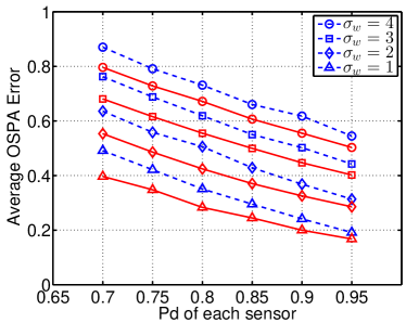
(a) Solid lines: G-CPHD; Dashed lines: G-PHD

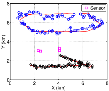
(b) Solid lines: True tracks; Dashed lines: Estimated tracks

Figure 6: (a): Average OSPA error Vs probability of detection of individual sensors. Different plots obtained by changing $\sigma_{w}$ in the range $\{1,2,3,4\}$. Blue dashed curves correspond to G-PHD filter and red solid curves correspond to G-CPHD filter. (b): True target tracks (solid red) and estimated target tracks (dashed with markers) obtained using the G-CPHD filter when $\sigma_{w}=2$ and $p_{d}=0.9$.

VII Conclusions

In this paper we address the problem of multitarget tracking using multiple sensors. Many of the existing approaches do not make complete use of the multisensor information or are computationally infeasible. The contribution of this work is twofold. As our first contribution we derive update equations for the general multisensor CPHD filter. These update equations, similar to the general multisensor PHD filter update equations, are combinatorial in nature and hence computationally intractable. Our second contribution is in developing an approximate greedy implementation of the general multisensor CPHD and PHD filters based on a Gaussian mixture model. The algorithm avoids any combinatorial calculations without sacrificing tracking accuracy. The algorithm is also scalable since the computational requirements grow linearly in the number of sensors as observed from the simulations.

Appendix A Recursive expression for partitions

Let ${\cal P}^{({\ell})}$ be the collection of all permissible partitions of the set $Z^{1:{\ell}}_{k+1}$ ($1\leq{\ell}<s$) where partitions are as defined in the equations (11)-(14). Since the $V$ component of a partition is unique given the $W$ components, we do not explicitly specify the $V$ component in the recursive expression. Let $P\in{\cal P}^{({\ell})}$ be any partition of $Z^{1:{\ell}}_{k+1}$ which is given as $P=\{W_{1},W_{2},\dots,,W_{|P|-1},V\}$. Let $Z^{{\ell}+1}_{k+1}=\{{\mathbf{z}}^{{\ell}+1}_{1},{\mathbf{z}}^{{\ell}+1}_{2},\dots,{\mathbf{z}}^{{\ell}+1}_{m_{{\ell}+1}}\}$. Then we can express ${\cal P}^{({\ell}+1)}$ using ${\cal P}^{({\ell})}$ and $Z^{{\ell}+1}$ as given by the following relation

$${\cal P}^{({\ell}+1)}=$$

$$\bigcup_{P\in{\cal P}^{({\ell})}}\bigcup_{n_{1}=0}^{m_{{\ell}+1}}\bigcup_{n_{2}=0}^{\textrm{min}(m_{{\ell}+1},|P|-1)}\!\!\!\!\!\!\bigcup_{\begin{subarray}{c}I_{1}\subseteq{\lsem}1,m_{{\ell}+1}{\rsem}\\ |I_{1}|=n_{1}\end{subarray}}\bigcup_{\begin{subarray}{c}I_{2}\subseteq{\lsem}1,m_{{\ell}+1}{\rsem}\\ |I_{2}|=n_{2}\\ I_{1}\cap I_{2}=\emptyset\end{subarray}}\bigcup_{\begin{subarray}{c}J\subseteq{\lsem}1,|P|-1{\rsem}\\ |J|=|I_{2}|\end{subarray}}$$

$$\quad\bigcup_{B\in\mathcal{B}(I_{2},J)}\left\{\{{\mathbf{z}}^{{\ell}+1}_{i_{1}}\}_{i_{1}\in I_{1}}\cup\{W_{B(i_{2})},{\mathbf{z}}^{{\ell}+1}_{i_{2}}\}_{i_{2}\in I_{2}}\cup\{W_{j}\}_{j\notin J}\right\}$$ (52)

where $\mathcal{B}(I_{2},J)$ is the collection of all possible matchings  from set $I_{2}$ to set $J$. The above relation mathematically expresses the fact that for each partition $P\in{\cal P}^{({\ell})}$ and given $Z^{{\ell}+1}_{k+1}$, a new partition belonging to ${\cal P}^{({\ell}+1)}$ can be constructed by adding some new singleton measurement subsets from $Z^{{\ell}+1}_{k+1}$ (i.e. $\{{\mathbf{z}}^{{\ell}+1}_{i_{1}}\}_{i_{1}\in I_{1}}$), extending some existing subsets in $P$ by appending them with measurements from $Z^{{\ell}+1}_{k+1}$ (i.e. $\{W_{B(i_{2})}\cup{\mathbf{z}}^{{\ell}+1}_{i_{2}}\}_{i_{2}\in I_{2}}$) and retaining some existing measurement subsets (i.e. $\{W_{j}\}_{j\notin J}$). By this definition we have ${\cal P}={\cal P}^{(s)}$. As a special case for ${\ell}=1$,

$${\cal P}^{(1)} =\bigcup_{n=0}^{m_{1}}\bigcup_{\begin{subarray}{c}I\subseteq{\lsem}1,m_{1}{\rsem}\\ |I|=n\end{subarray}}\left\{\{{\mathbf{z}}^{1}_{i}\}_{i\in I}\right\}.$$ (53)

Appendix B Functional derivatives

We now review the notion of functional derivatives which play an important role in the derivation of filter update equations. A brief background is provided that is necessary for the derivations in this paper; for additional details see [4], [2, Ch. 11], [17]. Let ${\mathcal{F}}$ denote the set of mappings from ${\cal Y}$ to ${\mathbb{R}}$ and let $A$ be a functional mapping elements of ${\mathcal{F}}$ to ${\mathbb{R}}$. Let $u({\mathbf{y}})$ and $g({\mathbf{y}})$ be functions in ${\mathcal{F}}$. For the functional $A[u]$, its Gâteaux derivative along the direction of the function $g({\mathbf{y}})$ is defined as [2]

$$\frac{\partial A}{\partial g}[u]\,\mathrel{\overset{\makebox[0.0pt]{\mbox{\tiny def}}}{=}}\,\lim_{\epsilon\rightarrow 0}\frac{A[u+\epsilon\cdot g]-A[u]}{\epsilon}.$$ (54)

In this paper we are interested in the Gâteaux derivatives when the function $g({\mathbf{y}})$ is the Dirac delta function $\delta_{{\mathbf{y}}_{1}}({\mathbf{y}})$ localized at ${\mathbf{y}}_{1}$ and the corresponding Gâteaux derivatives are called functional derivatives [2, 4]. In this case, the functional derivative is commonly written,

$$\frac{\partial A}{\partial\delta_{{\mathbf{y}}_{1}}}[u]\equiv\frac{\delta A}{\delta{\mathbf{y}}_{1}}[u].$$ (55)

If the functional $A[u]$ is of the form $A[u]=\int\!{u({\mathbf{y}})g({\mathbf{y}})d{\mathbf{y}}}$ then we have $\frac{\delta A}{\delta{\mathbf{y}}_{1}}[u]=g({\mathbf{y}}_{1})$.

We can also define higher order functional derivatives of $A[u]$. For a set $Y=\{{\mathbf{y}}_{1},{\mathbf{y}}_{2},\cdots,{\mathbf{y}}_{n}\}$, the $n^{th}$ order derivative is denoted by

$$\frac{\delta^{n}A}{\delta Y}[u] \mathrel{\overset{\makebox[0.0pt]{\mbox{\tiny def}}}{=}}\frac{\delta^{n}A}{\delta{\mathbf{y}}_{1}\delta{\mathbf{y}}_{2}\dots\delta{\mathbf{y}}_{n}}[u].$$ (56)

We call $\frac{\delta^{n}A}{\delta Y}[u]$ the functional derivative of $A[u]$ with respect to the set $Y$.

For functionals $A_{1}[u]$, $A_{2}[u]$ and $A_{3}[u]$, the product rule for functional derivatives [2, Ch. 11] gives

$$\frac{\delta}{\delta Y}\{A_{1}[u]\,A_{2}[u]\,A_{3}[u]\}$$

$$=\sum_{Y_{1}\subseteq Y}\sum_{\begin{subarray}{c}Y_{2}\subseteq Y\\ Y_{1}\cap Y_{2}=\emptyset\end{subarray}}\frac{\delta A_{1}}{\delta Y_{1}}[u]\frac{\delta A_{2}}{\delta Y_{2}}[u]\frac{\delta A_{3}}{\delta(Y-Y_{1}-Y_{2})}[u]$$ (57)

$$=\sum_{n_{1}=0}^{|Y|}\sum_{n_{2}=0}^{|Y|}\sum_{\begin{subarray}{c}Y_{1}\subseteq Y\\ |Y_{1}|=n_{1}\end{subarray}}\sum_{\begin{subarray}{c}Y_{2}\subseteq Y\\ |Y_{2}|=n_{2}\\ Y_{1}\cap Y_{2}=\emptyset\end{subarray}}\frac{\delta A_{1}}{\delta Y_{1}}[u]\frac{\delta A_{2}}{\delta Y_{2}}[u]\frac{\delta A_{3}}{\delta(Y-Y_{1}-Y_{2})}[u].$$ (58)

As a special case, for the product of two functionals we have

$$\frac{\delta}{\delta Y}\{A_{1}[u]\,A_{2}[u]\} =\sum_{n=0}^{|Y|}\sum_{\begin{subarray}{c}Y_{1}\subseteq Y\\ |Y_{1}|=n\end{subarray}}\frac{\delta A_{1}}{\delta Y_{1}}[u]\frac{\delta A_{2}}{\delta(Y-Y_{1})}[u].$$ (59)

Appendix C Probability generating functional

Let $u({\mathbf{x}})$ be a function with the mapping $u:\mathcal{X}\rightarrow[0,1]$, where $\mathcal{X}$ is the single target state space. For a set $X\subseteq\mathcal{X}$, define $u^{X}\mathrel{\overset{\makebox[0.0pt]{\mbox{\tiny def}}}{=}}\prod_{{\mathbf{x}}\in X}{u({\mathbf{x}})}$. Let $\Xi$ be a random finite set with elements in $\mathcal{X}$ and let $f_{\Xi}(X)$ be its probability density function. The probability generating functional (PGFL [2]) of the random finite set $\Xi$ is defined as the following integral transform

$$G_{\Xi}[u] \mathrel{\overset{\makebox[0.0pt]{\mbox{\tiny def}}}{=}}\int{u^{X}\;f_{\Xi}(X)\delta X}$$ (60)

where the integration is a set integral [2].

For a constant $a\in[0,1]$ denote by $u({\mathbf{x}})\equiv a$ the constant function $u({\mathbf{x}})=a$, for all ${\mathbf{x}}\in\mathcal{X}$. Let $A[a]$ denote the value of the functional $A[u]$ evaluated at $u({\mathbf{x}})\equiv a$. Recall that for a random variable its moments are related to the derivatives of its PGF. Similarly, the first moment or the PHD function of a random finite set is related to the functional derivative of its PGFL. For the random finite set $\Xi$, its PHD function $D_{\Xi}({\mathbf{x}})$ is related to the functional derivative of the PGFL [2] as follows

$$D_{\Xi}({\mathbf{x}})=\frac{\delta G_{\Xi}}{\delta{\mathbf{x}}}[1].$$ (61)

The PGF ${M}_{\Xi}(t)$ of the cardinality distribution of the random finite set $\Xi$ is obtained by substituting the constant function $u({\mathbf{x}})\equiv t$, in the PGFL i.e., ${M}_{\Xi}(t)=G_{\Xi}[t]$. For an IIDC random finite set with spatial density function $\zeta({\mathbf{x}})$ we have the relation $G_{\Xi}[u]={M}_{\Xi}(\langle\zeta,u\rangle)$.

Appendix D Multitarget Bayes filter

Let $f_{k+1|k}(X|Z^{1:s}_{1:k})$ and $f_{k+1|k+1}(X|Z^{1:s}_{1:k+1})$ be the predicted and posterior multitarget state distributions at time $k+1$ and let $L_{k+1,j}(Z^{j}_{k+1}|X)$ denote the multitarget likelihood function for the $j^{th}$ sensor at time $k+1$. Since the sensor observations are independent conditional on the multitarget state, the update equation for the multitarget Bayes filter [2] is given by

$$f_{k+1|k+1}(X|Z^{1:s}_{1:k+1}) \propto f_{k+1|k}(X|Z^{1:s}_{1:k})\prod_{j=1}^{s}{L_{k+1,j}(Z^{j}_{k+1}|X)}.$$ (62)

We now define a multivariate functional which is the integral transform of the quantity in the right hand side of the above equation. Under the conditions of Assumption 1, we can obtain a closed form expression for this multivariate functional, which on differentiation gives the PGFL of the posterior multitarget state distribution.

Let $g_{j}({\mathbf{z}}),j=1,2,\dots,s$ be functions that map the space $\mathcal{Z}^{j}$ to $[0,1]$ where $\mathcal{Z}^{j}$ is the space of observations of sensor $j$. The intermediate functions $g_{j}({\mathbf{z}})$ will be used to define functionals and later set to zero to obtain the PGFL of the posterior multitarget distribution. Let $u({\mathbf{x}})$ be a function mapping the state space $\mathcal{X}$ to $[0,1]$. For brevity, denote the vector of functions $[g_{1},g_{2},\dots,g_{s}]$ as $g_{1:s}$ and define $g_{j}^{Z^{j}}\mathrel{\overset{\makebox[0.0pt]{\mbox{\tiny def}}}{=}}\prod_{{\mathbf{z}}\in Z^{j}}{g_{j}({\mathbf{z}})}$ where $Z^{j}\subseteq\mathcal{Z}^{j}$. We define the multivariate functional $F[g_{1},g_{2},\dots,g_{s},u]$ as the following integral transform

$$F[g_{1:s},u]\mathrel{\overset{\makebox[0.0pt]{\mbox{\tiny def}}}{=}}\int{u^{X}\,\left(\prod_{j=1}^{s}{\mathcal{L}_{k+1,j}[g_{j}|X]}\right)\,f_{k+1|k}(X|Z^{1:s}_{1:k})\,\delta X}$$ (63)

$$\text{where }\mathcal{L}_{k+1,j}[g_{j}|X]\mathrel{\overset{\makebox[0.0pt]{\mbox{\tiny def}}}{=}}\int{g_{j}^{Z^{j}}\,L_{k+1,j}(Z^{j}|X)\delta Z^{j}}.$$ (64)

Later we will relate the PGFL of the posterior multitarget distribution to the derivatives of the functional $F[g_{1:s},u]$ with respect to the sensor observations $Z^{1:s}_{k+1}$. Recall that $c_{j}({\mathbf{z}})$ denotes the clutter spatial distribution and $C_{j}(t)$ denotes the PGF of the clutter cardinality distribution for the $j^{th}$ sensor. Under Assumption 1 it can be shown that [3]

$$\mathcal{L}_{k+1,j}[g_{j}|X] =\int{g_{j}^{Z^{j}}\,L_{k+1,j}(Z^{j}|X)\delta Z^{j}}$$ (65)

$$=C_{j}(\langle c_{j},g_{j}\rangle)\,\phi_{g_{j}}^{X}\,,$$ (66)

$$\textrm{where }\phi_{g_{j}}({\mathbf{x}}) \mathrel{\overset{\makebox[0.0pt]{\mbox{\tiny def}}}{=}}1-p^{j}_{d}({\mathbf{x}})+p^{j}_{d}({\mathbf{x}})\,p_{g_{j}}({\mathbf{x}})$$ (67)

$$p_{g_{j}}({\mathbf{x}}) \mathrel{\overset{\makebox[0.0pt]{\mbox{\tiny def}}}{=}}\int{g_{j}({\mathbf{z}})h_{j}({\mathbf{z}}|{\mathbf{x}})d{\mathbf{z}}}.$$ (68)

Let $G_{k+1|k}[u]$ denote the PGFL of the predicted multitarget distribution. Using the above relations in (63) we have

$$F[ g_{1:s},u]=\int\!\!{u^{X}\,\left(\prod_{j=1}^{s}{C_{j}(\langle c_{j},g_{j}\rangle)}\,\phi_{g_{j}}^{X}\right)\,f_{k+1|k}(X|Z^{1:s}_{1:k})\,\delta X}$$ (69)

Since both $u$ and $\phi_{g_{j}}$ are functions defined over the space $\mathcal{X}$, we can combine the product of $u^{X}$ and $\prod_{j=1}^{s}{\phi_{g_{j}}^{X}}$ and write $(u\,\prod_{j=1}^{s}{\phi_{g_{j}}})^{X}$. Hence we have

$$F[g_{1:s},u]$$

$$=\left(\prod_{j=1}^{s}{C_{j}(\langle c_{j},g_{j}\rangle)}\right)\,\int{\left(u\,\prod_{j=1}^{s}{\phi_{g_{j}}}\right)^{X}\,f_{k+1|k}(X|Z^{1:s}_{1:k})\,\delta X}$$ (70)

$$=\left(\prod_{j=1}^{s}{C_{j}(\langle c_{j},g_{j}\rangle)}\right)\,G[u\prod_{j=1}^{s}{\phi_{g_{j}}}]$$ (71)

$$=\left(\prod_{j=1}^{s}{C_{j}(\langle c_{j},g_{j}\rangle)}\right)\,{M}(\langle r,u\prod_{j=1}^{s}{\phi_{g_{j}}}\rangle).$$ (72)

The last two steps result from the definition of the PGFL and the assumption that the predicted multitarget distribution $f_{k+1|k}(X|Z^{1:s}_{1:k})$ is IIDC.

Let $G_{k+1|k+1}[u]$ be the PGFL of the multitarget density $f_{k+1|k+1}(X|Z^{1:s}_{1:k+1})$, and let $D_{k+1|k+1}({\mathbf{x}})$ be the posterior PHD function. From [8, 10] we have the following relation

$$G_{k+1|k+1}[u] =\frac{\displaystyle\frac{\delta F}{\delta Z^{1:s}_{k+1}}[0,0,\dots,0,u]}{\displaystyle\frac{\delta F}{\delta Z^{1:s}_{k+1}}[0,0,\dots,0,1]}.$$ (73)

Since the PHD is the functional derivative of the PGFL, from (61)

$$D_{k+1|k+1}({\mathbf{x}}) =\frac{\displaystyle\frac{\delta F}{\delta{\mathbf{x}}\,\delta Z^{1:s}_{k+1}}[0,0,\dots,0,1]}{\displaystyle\frac{\delta F}{\delta Z^{1:s}_{k+1}}[0,0,\dots,0,1]}.$$ (74)

Note that the differentiation $\frac{\delta}{\delta Z^{j}_{k+1}}$ is with respect to the function variable $g_{j}$ and the differentiation $\frac{\delta}{\delta{\mathbf{x}}}$ is with respect to the function variable $u$. The general multisensor CPHD filter update equation is derived by evaluating the functional derivatives of $F[g_{1:s},u]$ in (73) and (74).

We now define a quantity $\Gamma$ and the functionals $\Psi_{P}[g_{1:s},u]$ and $\varphi_{W}[g_{1:s},u]$. The functional derivatives of $F[g_{1:s},u]$ can be expressed in terms of these quantities. Let

$$\Gamma \mathrel{\overset{\makebox[0.0pt]{\mbox{\tiny def}}}{=}}\prod_{j=1}^{s}{\left(\prod_{{\mathbf{z}}\in Z^{j}_{k+1}}{c_{j}({\mathbf{z}})}\right)},$$ (75)

$$\Psi_{P} [g_{1:s},u]$$

$$\mathrel{\overset{\makebox[0.0pt]{\mbox{\tiny def}}}{=}}\left(\prod_{j=1}^{s}{C^{(m_{j}-|P|_{j})}_{j}(\langle c_{j},g_{j}\rangle)}\right)\,{M}^{(|P|-1)}(\langle r,u\prod_{j=1}^{s}{\phi_{g_{j}}}\rangle).$$ (76)

For $W\in\mathcal{W}$, let

$$\varphi_{W}[g_{1:s},u]$$

$$\mathrel{\overset{\makebox[0.0pt]{\mbox{\tiny def}}}{=}}\frac{\displaystyle\int\!\!r({\mathbf{x}})u({\mathbf{x}})\left(\prod_{(i,l)\in T_{W}}{\!\!\!\!p_{d}^{i}({\mathbf{x}})\,h_{i}({\mathbf{z}}^{i}_{l}|{\mathbf{x}})}\right)\,\left(\prod_{j:(j,*)\notin T_{W}}{\!\!\!\!\!\!\phi_{g_{j}({\mathbf{x}})}}\right)d{\mathbf{x}}}{\displaystyle\prod_{(i,l)\in T_{W}}{c_{i}({\mathbf{z}}^{i}_{l})}}\cdot$$ (77)

With these definitions we can prove, via mathematical induction, the following lemma.

Lemma 1.

Under the conditions of Assumption 1, the functional derivative of $F[g_{1:s},u]$ with respect to the multisensor observation set $Z^{1:s}_{k+1}$ is given by

$$\frac{\delta F}{\delta Z^{1:s}_{k+1}}[g_{1:s},u] =\Gamma\sum_{P\in{\cal P}}\Psi_{P}[g_{1:s},u]\prod_{W\in P}{\varphi_{W}[g_{1:s},u]}$$ (78)

where $\Gamma$, $\Psi_{P}[g_{1:s},u]$ and $\varphi_{W}[g_{1:s},u]$ are as defined in (75), (76) and (77).

Lemma 1 is proved in Appendix E.

Appendix E Proof of Lemma 1

Proof.

The derivation is based on the approach used by Mahler [8] to derive multisensor PHD filter equations for the two sensor case and its extension by Delande et al. [10] for the general case of $s$ sensors.

Mathematical induction

We prove using mathematical induction on $1\leq{\ell}\leq s$ the following result,

$$\frac{\delta F}{\delta Z^{1:{\ell}}_{k+1}}[g_{1:s},u] =\Gamma^{({\ell})}\sum_{P\in{\cal P}^{({\ell})}}\Psi_{P}^{({\ell})}[g_{1:s},u]\prod_{W\in P}{\varphi_{W}[g_{1:s},u]}$$ (79)

where,

$$\Gamma^{({\ell})} \mathrel{\overset{\makebox[0.0pt]{\mbox{\tiny def}}}{=}}\prod_{j=1}^{{\ell}}{\prod_{{\mathbf{z}}\in Z^{j}_{k+1}}{c_{j}({\mathbf{z}})}},$$ (80)

$$\Psi_{P}^{({\ell})} [g_{1:s},u]\mathrel{\overset{\makebox[0.0pt]{\mbox{\tiny def}}}{=}}\left(\prod_{j=1}^{{\ell}}{C^{(m_{j}-|P|_{j})}_{j}(\langle c_{j},g_{j}\rangle)}\right)$$

$$\times\left(\prod_{j={\ell}+1}^{s}{C_{j}(\langle c_{j},g_{j}\rangle)}\right)\times{M}^{(|P|-1)}(\langle r,u\prod_{j=1}^{s}{\phi_{g_{j}}}\rangle),$$ (81)

and for $W\in\mathcal{W}$,

$$\varphi_{W}[g_{1:s},u]$$

$$\mathrel{\overset{\makebox[0.0pt]{\mbox{\tiny def}}}{=}}\frac{\displaystyle\int\!\!r({\mathbf{x}})u({\mathbf{x}})\left(\prod_{(i,l)\in T_{W}}{\!\!\!\!p_{d}^{i}({\mathbf{x}})\,h_{i}({\mathbf{z}}^{i}_{l}|{\mathbf{x}})}\right)\,\left(\prod_{j:(j,*)\notin T_{W}}{\!\!\!\!\!\phi_{g_{j}({\mathbf{x}})}}\right)d{\mathbf{x}}}{\displaystyle\prod_{(i,l)\in T_{W}}{c_{i}({\mathbf{z}}^{i}_{l})}}\cdot$$ (82)

Mathematical induction: case ${\ell}=1$

We first establish the induction result for the base case, i.e. ${\ell}=1$. Ignoring the time index let the observation set gathered by sensor 1 at time $k+1$ be $Z^{1}_{k+1}=\{{\mathbf{z}}^{1}_{1},{\mathbf{z}}^{1}_{2},\dots,{\mathbf{z}}^{1}_{m_{1}}\}$. We have, for the case of $s$ sensors

$$F[g_{1:s},u] =\left(\prod_{j=1}^{s}{C_{j}(\langle c_{j},g_{j}\rangle)}\right)\,{M}(\langle r,u\prod_{j=1}^{s}{\phi_{g_{j}}}\rangle).$$ (83)

Differentiating the above expression with respect to the set $Z^{1}_{k+1}$ we get

$$\frac{\delta F}{\delta Z^{1}_{k+1}}[g_{1:s},u]$$

$$=\frac{\delta}{\delta Z^{1}_{k+1}}\left\{\left(\prod_{j=1}^{s}{C_{j}(\langle c_{j},g_{j}\rangle)}\right)\,{M}(\langle r,u\prod_{j=1}^{s}{\phi_{g_{j}}}\rangle)\right\}$$ (84)

$$=\left(\prod_{j=2}^{s}{C_{j}(\langle c_{j},g_{j}\rangle)}\right)\frac{\delta}{\delta Z^{1}_{k+1}}\left\{{C_{1}(\langle c_{1},g_{1}\rangle)}\,{M}(\langle r,u\prod_{j=1}^{s}{\phi_{g_{j}}}\rangle)\right\}$$ (85)

since the differential $\frac{\delta}{\delta Z^{1}_{k+1}}$ only differentiates the variable $g_{1}$. If $I\subseteq{\lsem}1,m_{1}{\rsem}$ we can express $Y\subseteq Z^{1}_{k+1}$ as $Y=\{{\mathbf{z}}^{1}_{i}:i\in I\}$ for some $I$. We also have $Z^{1}_{k+1}-Y=\{{\mathbf{z}}^{1}_{i}:i\notin I\}$. Using the product rule for functional derivatives from (59) we have

$$\frac{\delta}{\delta Z^{1}_{k+1}}\left\{{C_{1}(\langle c_{1},g_{1}\rangle)}\,{M}(\langle r,u\prod_{j=1}^{s}{\phi_{g_{j}}}\rangle)\right\}$$

$$=\sum_{n=0}^{m_{1}}\sum_{\begin{subarray}{c}I\subseteq{\lsem}1,m_{1}{\rsem}\\ |I|=n\end{subarray}}\frac{\delta}{\delta\{{\mathbf{z}}^{1}_{i}\}_{i\in I}}{M}(\langle r,u\prod_{j=1}^{s}{\phi_{g_{j}}}\rangle)\frac{\delta}{\delta\{{\mathbf{z}}^{1}_{i}\}_{i\notin I}}{C_{1}(\langle c_{1},g_{1}\rangle)}.$$ (86)

Now we consider the derivatives of each of the individual terms in the above expression. By application of the chain rule for functional derivatives [2, Ch. 11]

$$\frac{\delta}{\delta\{{\mathbf{z}}^{1}_{i}\}_{i\in I}}{M}(\langle r,u\prod_{j=1}^{s}{\phi_{g_{j}}}\rangle)$$

$$={M}^{(n)}(\langle r,u\prod_{j=1}^{s}{\phi_{g_{j}}}\rangle)\,\prod_{i\in I}{\langle r,u\,p^{1}_{d}\,h_{1}({\mathbf{z}}^{1}_{i})\,\prod_{j=2}^{s}{\phi_{g_{j}}}\rangle}.$$ (87)

In the expression above and in later expressions we have used the convention that whenever $|I|=0$, $\prod_{i\in I}()=1$. Applying the chain rule to the second derivative

$$\frac{\delta}{\delta\{{\mathbf{z}}^{1}_{i}\}_{i\notin I}}{C_{1}(\langle c_{1},g_{1}\rangle)} =C^{(m_{1}-n)}_{1}(\langle c_{1},g_{1}\rangle)\;\prod_{i\notin I}{c_{1}({\mathbf{z}}^{1}_{i})}$$ (88)

$$=C^{(m_{1}-n)}_{1}(\langle c_{1},g_{1}\rangle)\;\frac{\Gamma^{(1)}}{\displaystyle\prod_{i\in I}{c_{1}({\mathbf{z}}^{1}_{i})}}.$$ (89)

As before we have used the convention $\prod_{i\in I}()=1$ when $|I|=0$. Thus the right hand side of (86) can be expressed as

$$\Gamma^{(1)} \,\sum_{n=0}^{m_{1}}\sum_{\begin{subarray}{c}I\subseteq{\lsem}1,m_{1}{\rsem}\\ |I|=n\end{subarray}}\Bigg{\{}{M}^{(n)}(\langle r,u\prod_{j=1}^{s}{\phi_{g_{j}}}\rangle)\times$$

$$C^{(m_{1}-n)}_{1}(\langle c_{1},g_{1}\rangle)\prod_{i\in I}{\frac{\langle r,u\,p^{1}_{d}\,h_{1}({\mathbf{z}}^{1}_{i})\,\prod_{j=2}^{s}{\phi_{g_{j}}}\rangle}{c_{1}({\mathbf{z}}^{1}_{i})}}\Bigg{\}}.$$ (90)

In the double summation above, each set $I$ maps to a partition $P$ of the form $P=\bigcup_{i\in I}{\{{\mathbf{z}}^{1}_{i}\}}$ in ${\cal P}^{(1)}$ and vice versa. Hence using result in equation (53) of Appendix A we have

$$\frac{\delta F}{\delta Z^{1}_{k+1}}[g_{1:s},u]=\Gamma^{(1)}\sum_{P\in{\cal P}^{(1)}}\Bigg{\{}C^{(m_{1}-|P|_{1})}_{1}(\langle c_{1},g_{1}\rangle)\times$$

$$\left(\prod_{j=2}^{s}{C_{j}(\langle c_{j},g_{j}\rangle)}\right){M}^{(|P|-1)}(\langle r,u\prod_{j=1}^{s}{\phi_{g_{j}}}\rangle)\;\prod_{W\in P}{\varphi_{W}[g_{1:s},u]}\Bigg{\}}$$ (91)

Note that for the empty partition $P=\{V\}$, there are no elements of the form $W$ in $P$. Hence in the above expression we use the convention $\prod_{W\in P}()=1$ whenever $P=\{V\}$. Further grouping of the terms gives the compact expression

$$\frac{\delta F}{\delta Z^{1}_{k+1}}[g_{1:s},u]=\Gamma^{(1)}\sum_{P\in{\cal P}^{(1)}}\Psi_{P}^{(1)}[g_{1:s},u]\prod_{W\in P}{\varphi_{W}[g_{1:s},u]}.$$ (92)

Hence the result is established for the case ${\ell}=1$.
Mathematical induction: case ${\ell}=b\geq 1$

Now assuming that the result is true for some ${\ell}=b\geq 1$, we establish that the result holds for ${\ell}=b+1\leq s$. Let $Z^{b+1}_{k+1}=\{{\mathbf{z}}^{b+1}_{1},\,{\mathbf{z}}^{b+1}_{2},\dots,{\mathbf{z}}^{b+1}_{m_{b+1}}\}$. We can write

$$\frac{\delta F}{\delta Z^{1:b+1}_{k+1}}[g_{1:s},u] =\frac{\delta}{\delta Z^{b+1}_{k+1}}\left\{\frac{\delta F}{\delta Z^{1:b}_{k+1}}[g_{1:s},u]\right\}.$$ (93)

Substituting the result for the case ${\ell}=b$ we get

$$\frac{\delta F}{\delta Z^{1:b+1}_{k+1}}[g_{1:s},u]$$

$$=\frac{\delta}{\delta Z^{b+1}_{k+1}}\Bigg{\{}\Gamma^{(b)}\sum_{P\in{\cal P}^{(b)}}\Psi_{P}^{(b)}[g_{1:s},u]\prod_{W\in P}{\varphi_{W}[g_{1:s},u]}\Bigg{\}}$$ (94)

$$=\Gamma^{(b)}\left(\prod_{j=b+2}^{s}{C_{j}(\langle c_{j},g_{j}\rangle)}\right)\sum_{P\in{\cal P}^{(b)}}\left(\prod_{j=1}^{b}{C^{(m_{j}-|P|_{j})}_{j}(\langle c_{j},g_{j}\rangle)}\right)$$

$$\quad\times\frac{\delta}{\delta Z^{b+1}_{k+1}}\Bigg{\{}C_{b+1}(\langle c_{b+1},g_{b+1}\rangle){M}^{(|P|-1)}(\langle r,u\prod_{j=1}^{s}{\phi_{g_{j}}}\rangle)\times$$

$$\qquad\qquad\prod_{W\in P}{\varphi_{W}[g_{1:s},u]}\Bigg{\}}.$$ (95)

Let $I_{1}\subseteq{\lsem}1,m_{b+1}{\rsem}$ and $I_{2}\subseteq{\lsem}1,m_{b+1}{\rsem}$ such that $I_{1}\cap I_{2}=\emptyset$. Then we can express $Y_{1}\subseteq Z^{b+1}_{k+1}$ and $Y_{2}\subseteq Z^{b+1}_{k+1}$ satisfying $Y_{1}\cap Y_{2}=\emptyset$ as $Y_{1}=\{{\mathbf{z}}^{b+1}_{i}:i\in I_{1}\}$ and $Y_{2}=\{{\mathbf{z}}^{b+1}_{i}:i\in I_{2}\}$ respectively. Applying the product rule from (58) to the expression above we have

$$\frac{\delta}{\delta Z^{b+1}_{k+1}}\Bigg{\{}C_{b+1}(\langle c_{b+1},g_{b+1}\rangle){M}^{(|P|-1)}(\langle r,u\prod_{j=1}^{s}{\phi_{g_{j}}}\rangle)\times$$

$$\qquad\qquad\prod_{W\in P}{\varphi_{W}[g_{1:s},u]}\Bigg{\}}$$

$$\;=\sum_{n_{1}=0}^{m_{b+1}}\sum_{n_{2}=0}^{\textrm{min}(m_{b+1},|P|-1)}\sum_{\begin{subarray}{c}I_{1}\subseteq{\lsem}1,m_{b+1}{\rsem}\\ |I_{1}|=n_{1}\end{subarray}}\sum_{\begin{subarray}{c}I_{2}\subseteq{\lsem}1,m_{b+1}{\rsem}\\ |I_{2}|=n_{2};\;I_{1}\cap I_{2}=\emptyset\end{subarray}}$$

$$\qquad\Bigg{\{}\frac{\delta}{\delta\{{\mathbf{z}}^{b+1}_{i_{1}}\}_{i_{1}\in I_{1}}}{M}^{(|P|-1)}(\langle r,u\prod_{n=1}^{s}{\phi_{g_{n}}}\rangle)\times$$

$$\qquad\qquad\frac{\delta}{\delta\{{\mathbf{z}}^{b+1}_{i_{2}}\}_{i_{2}\in I_{2}}}\left(\prod_{W\in P}{\varphi_{W}[g_{1:s},u]}\right)\times$$

$$\qquad\qquad\frac{\delta}{\delta\{{\mathbf{z}}^{b+1}_{i}\}_{i\notin I_{1}\cup I_{2}}}C_{b+1}(\langle c_{b+1},g_{b+1}\rangle)\Bigg{\}}.$$ (96)

The second summation above is restricted to the limit $\textrm{min}(m_{b+1},|P|-1)$ because the derivatives of $\prod_{W\in P}{\varphi_{W}[g_{1:s},u]}$ for $n_{2}>|P|-1$ are zero. Now considering each of the individual derivatives above we have

$$\frac{\delta}{\delta\{{\mathbf{z}}^{b+1}_{i_{1}}\}_{i_{1}\in I_{1}}}{M}^{(|P|-1)}(\langle r,u\prod_{n=1}^{s}{\phi_{g_{n}}}\rangle)$$

$$={M}^{(|P|+n_{1}-1)}(\langle r,u\prod_{n=1}^{s}{\phi_{g_{n}}}\rangle)\prod_{i_{1}\in I_{1}}{\varphi_{\{{\mathbf{z}}^{b+1}_{i_{1}}\}}[g_{1:s},u]\,c_{b+1}({\mathbf{z}}^{b+1}_{i_{1}})}.$$ (97)

Denote $P=\{W_{1},W_{2},\dots,W_{|P|-1},V\}$ for notational convenience. Then we have

$$\frac{\delta}{\delta\{{\mathbf{z}}^{b+1}_{i_{2}}\}_{i_{2}\in I_{2}}} \left(\prod_{W\in P}{\varphi_{W}[g_{1:s},u]}\right)$$

$$=\sum_{\begin{subarray}{c}J\subseteq{\lsem}1,|P|-1{\rsem}\\ |J|=|I_{2}|\end{subarray}}\sum_{B\in\mathcal{B}(I_{2},J)}\Bigg{\{}\left(\prod_{j\notin J}{\varphi_{W_{j}}[g_{1:s},u]}\right)\times$$

$$\qquad\left(\prod_{i_{2}\in I_{2}}{\varphi_{W^{B}_{i_{2}}}[g_{1:s},u]\,c_{b+1}({\mathbf{z}}^{b+1}_{i_{2}})}\right)\Bigg{\}}$$ (98)

where $\mathcal{B}(I_{2},J)$ is the collection of all possible matchings from set $I_{2}$ to set $J$ and we define the measurement subset $W^{B}_{i_{2}}\mathrel{\overset{\makebox[0.0pt]{\mbox{\tiny def}}}{=}}W_{B(i_{2})}\cup{\mathbf{z}}^{b+1}_{i_{2}}$. Also

$$\frac{\delta}{\delta\{{\mathbf{z}}^{b+1}_{i}\}_{i\notin I_{1}\cup I_{2}}}\left(C_{b+1}(\langle c_{b+1},g_{b+1}\rangle)\right)$$

$$=C^{(m_{b+1}-n_{1}-n_{2})}_{b+1}(\langle c_{b+1},g_{b+1}\rangle)\prod_{i\notin I_{1}\cup I_{2}}{c_{b+1}({\mathbf{z}}^{b+1}_{i})}.$$ (99)

Combining the three derivatives into the right hand side of expression (95) we get

$$\Gamma^{(b)}\left(\prod_{j=b+2}^{s}{C_{j}(\langle c_{j},g_{j}\rangle)}\right)\left(\prod_{{\mathbf{z}}^{b+1}\in Z^{b+1}_{k+1}}{\!\!\!\!c_{b+1}({\mathbf{z}}^{b+1})}\right)$$

$$\sum_{P\in{\cal P}^{(b)}}\sum_{n_{1}=0}^{m_{b+1}}\sum_{n_{2}=0}^{\textrm{min}(m_{b+1},|P|-1)}\!\!\!\!\!\!\sum_{\begin{subarray}{c}I_{1}\subseteq{\lsem}1,m_{b+1}{\rsem}\\ |I_{1}|=n_{1}\end{subarray}}\sum_{\begin{subarray}{c}I_{2}\subseteq{\lsem}1,m_{b+1}{\rsem}\\ |I_{2}|=n_{2};\;I_{1}\cap I_{2}=\emptyset\end{subarray}}\sum_{\begin{subarray}{c}J\subseteq{\lsem}1,|P|-1{\rsem}\\ |J|=|I_{2}|\end{subarray}}$$

$$\sum_{B\in\mathcal{B}(I_{2},J)}\Bigg{\{}C^{(m_{b+1}-n_{1}-n_{2})}_{b+1}(\langle c_{b+1},g_{b+1}\rangle)\left(\prod_{j\notin J}{\varphi_{W_{j}}[g_{1:s},u]}\right)\times$$

$$\quad{M}^{(|P|+n_{1}-1)}(\langle r,u\prod_{n=1}^{s}{\phi_{g_{n}}}\rangle)\,\left(\prod_{j=1}^{b}{C^{(m_{j}-|P|_{j})}_{j}(\langle c_{j},g_{j}\rangle)}\right)\times$$

$$\quad\left(\prod_{i_{1}\in I_{1}}{\varphi_{\{{\mathbf{z}}^{b+1}_{i_{1}}\}}[g_{1:s},u]}\right)\left(\prod_{i_{2}\in I_{2}}{\varphi_{W^{B}_{i_{2}}}[g_{1:s},u]}\right)\Bigg{\}}.$$ (100)

Using result of Appendix A we can simplify the multiple summation term and write

$$\frac{\delta F}{\delta Z^{1:b+1}_{k+1}}[g_{1:s},u]=\Gamma^{(b+1)}\!\!\!\!\sum_{P\in{\cal P}^{(b+1)}}\Bigg{\{}\left(\prod_{j=1}^{b+1}{C^{(m_{j}-|P|_{j})}_{j}(\langle c_{j},g_{j}\rangle)}\right)$$

$$\qquad\left(\prod_{j=b+2}^{s}{C_{j}(\langle c_{j},g_{j}\rangle)}\right){M}^{(|P|+n_{1}-1)}(\langle r,u\prod_{n=1}^{s}{\phi_{g_{n}}}\rangle)\times$$

$$\qquad\left(\prod_{W\in P}{\varphi_{W}[g_{1:s},u]}\right)\Bigg{\}}$$

$$=\Gamma^{(b+1)}\sum_{P\in{\cal P}^{(b+1)}}\Psi_{P}^{(b+1)}[g_{1:s},u]\prod_{W\in P}{\varphi_{W}[g_{1:s},u]}.$$ (101)

Hence we have established the result stated in (79) using the method of mathematical induction. We obtain the result of Lemma 1 by substituting ${\ell}=s$ in this result.

∎

Appendix F Proof of Theorem 1

For brevity denote $\Psi_{P}[0,0,\dots,0,u]=\Psi_{P}[u]$ and $\varphi_{W}[0,0,\dots,0,u]=\varphi_{W}[u]$. Substituting $g_{j}\equiv 0$ for $j=1,2,\dots,s$ in the result of Lemma 1 we get

$$\frac{\delta F}{\delta Z^{1:s}_{k+1}}[0,0,\dots,0,u] =\Gamma\sum_{P\in{\cal P}}\Psi_{P}[u]\prod_{W\in P}{\varphi_{W}[u]}.$$ (102)

PHD update

Differentiating equation (102) with respect to set $\{{\mathbf{x}}\}$ we have

$$\frac{\delta F}{\delta{\mathbf{x}}\delta Z^{1:s}_{k+1}}[0,0,\dots,0,u]=\frac{\delta}{\delta{\mathbf{x}}}\left\{\frac{\delta F}{\delta Z^{1:s}_{k+1}}[0,0,\dots,0,u]\right\}$$ (103)

$$=\frac{\delta}{\delta{\mathbf{x}}}\left\{\Gamma\sum_{P\in{\cal P}}\Psi_{P}[u]\prod_{W\in P}{\varphi_{W}[u]}\right\}$$ (104)

$$=\Gamma\sum_{P\in{\cal P}}\left(\prod_{j=1}^{s}{C^{(m_{j}-|P|_{j})}_{j}(0)}\right)\times$$

$$\qquad\frac{\delta}{\delta{\mathbf{x}}}\left\{{M}^{(|P|-1)}(\langle r,u\prod_{j=1}^{s}{q^{j}_{d}}\rangle)\,\prod_{W\in P}{\varphi_{W}[u]}\right\}.$$ (105)

Applying the product rule for set derivatives from (59)

$$\frac{\delta}{\delta{\mathbf{x}}} \left\{{M}^{(|P|-1)}(\langle r,u\prod_{j=1}^{s}{q^{j}_{d}}\rangle)\,\prod_{W\in P}{\varphi_{W}[u]}\right\}$$

$$=\frac{\delta}{\delta{\mathbf{x}}}\left\{{M}^{(|P|-1)}(\langle r,u\prod_{j=1}^{s}{q^{j}_{d}}\rangle)\right\}\,\prod_{W\in P}{\varphi_{W}[u]}+$$

$$\quad{M}^{(|P|-1)}(\langle r,u\prod_{j=1}^{s}{q^{j}_{d}}\rangle)\frac{\delta}{\delta{\mathbf{x}}}\left\{\prod_{W\in P}{\varphi_{W}[u]}\right\}.$$ (106)

Evaluating the individual derivatives above and substituting the constant function $u({\mathbf{x}})\equiv 1$, we get

$$\frac{\delta}{\delta{\mathbf{x}}}\left\{{M}^{(|P|-1)}(\langle r,u\prod_{j=1}^{s}{q^{j}_{d}}\rangle)\right\}_{u\equiv 1}={M}^{(|P|)}(\gamma)\,r({\mathbf{x}})\prod_{j=1}^{s}{q^{j}_{d}({\mathbf{x}})}$$ (107)

$$\frac{\delta}{\delta{\mathbf{x}}}\left\{\prod_{W\in P}{\varphi_{W}[u]}\right\}_{u\equiv 1}=\left(\prod_{W\in P}{d_{W}}\right)\left(\sum_{W\in P}r({\mathbf{x}})\rho_{W}({\mathbf{x}})\right)$$ (108)

where $\gamma$, $d_{W}$ and $\rho_{W}({\mathbf{x}})$ are defined in (17), (19) and (20) respectively. We note that for the empty partition $P=\{V\}$ there are no elements of the form $W$ in $P$. In this case the derivative in equation (108) is zero since the quantity being differentiated is a constant equal to 1. To have a compact representation of the update equations we use the convention $\sum_{W\in P}()=0$ when $P=\{V\}$. Hence we have

$$\frac{\delta F}{\delta{\mathbf{x}}\delta Z^{1:s}_{k+1}}[0,0,\dots,0,1]=\Gamma\sum_{P\in{\cal P}}\left(\prod_{j=1}^{s}{C^{(m_{j}-|P|_{j})}_{j}(0)}\right)\times$$

$$\quad\Bigg{\{}{M}^{(|P|)}(\gamma)\,r({\mathbf{x}})\prod_{j=1}^{s}{q^{j}_{d}({\mathbf{x}})}\left(\prod_{W\in P}{d_{W}}\right)+$$

$$\qquad{M}^{(|P|-1)}(\gamma)\left(\prod_{W\in P}{d_{W}}\right)\left(\sum_{W\in P}{r({\mathbf{x}})\rho_{W}({\mathbf{x}})}\right)\Bigg{\}}$$ (109)

$$=\Gamma\sum_{P\in{\cal P}}\left(\kappa_{P}{M}^{(|P|)}\prod_{W\in P}{d_{W}}\right)\,\left(r({\mathbf{x}})\prod_{j=1}^{s}{q^{j}_{d}({\mathbf{x}})}\right)$$

$$\quad+\Gamma\sum_{P\in{\cal P}}\left(\kappa_{P}{M}^{(|P|-1)}\prod_{W\in P}{d_{W}}\right)\,\left(\sum_{W\in P}{r({\mathbf{x}})\,\rho_{W}({\mathbf{x}})}\right)$$ (110)

where $\kappa_{P}$ is defined in (18). Substituting $u({\mathbf{x}})\equiv 1$ in equation (102) we have

$$\frac{\delta F}{\delta Z^{1:s}_{k+1}}[0,0,\dots,0,1] =\Gamma\sum_{P\in{\cal P}}\kappa_{P}{M}^{(|P|-1)}\prod_{W\in P}{d_{W}}.$$ (111)

Dividing (110) by (111) and using the definition of PHD from (74), we get

$$D_{k+1|k+1}({\mathbf{x}})=\frac{\displaystyle\frac{\delta F}{\delta{\mathbf{x}}\delta Z^{1:s}_{k+1}}[0,0,\dots,0,1]}{\displaystyle\frac{\delta F}{\delta Z^{1:s}_{k+1}}[0,0,\dots,0,1]}$$ (112)

$$\quad=r({\mathbf{x}})\left\{\alpha_{0}\,\prod_{j=1}^{s}{q^{j}_{d}({\mathbf{x}})}+\sum_{P\in{\cal P}}\alpha_{P}\,\left(\sum_{W\in P}\rho_{W}({\mathbf{x}})\right)\right\}$$ (113)

where $\alpha_{0}$ and $\alpha_{P}$ are as given in (21) and (22).

Cardinality update

We now derive the update equation for the posterior cardinality distribution. Using the expression for the posterior probability generating functional in (73) and the results of (102) and (111) we have

$$G_{k+1|k+1}[u] =\frac{\displaystyle\sum_{P\in{\cal P}}\Psi_{P}[u]\prod_{W\in P}{\varphi_{W}[u]}}{\displaystyle\sum_{P\in{\cal P}}\kappa_{P}{M}^{(|P|-1)}\prod_{W\in P}{d_{W}}}.$$ (114)

The probability generating function ${M}_{k+1|k+1}(t)$ of the posterior cardinality distribution is obtained by substituting the constant function $u({\mathbf{x}})\equiv t$ in the expression for $G_{k+1|k+1}[u]$. Thus

$${M}_{k+1|k+1}(t) =\frac{\displaystyle\sum_{P\in{\cal P}}\Psi_{P}[t]\prod_{W\in P}{\varphi_{W}[t]}}{\displaystyle\sum_{P\in{\cal P}}\kappa_{P}{M}^{(|P|-1)}\prod_{W\in P}{d_{W}}}.$$ (115)

For constant $t$ we have

$$\displaystyle\prod_{W\in P}{\varphi_{W}[t]} =t^{|P|-1}\prod_{W\in P}{d_{W}}$$ (116)

$$\text{and }\Psi_{P}[t] =\left(\prod_{j=1}^{s}{C^{(m_{j}-|P|_{j})}_{j}(0)}\right){M}^{(|P|-1)}(t\gamma).$$ (117)

Since ${M}_{k+1|k+1}(t)$ is the PGF corresponding to the cardinality distribution $p_{k+1|k+1}(n)$,

$$p_{k+1|k+1}(n)=\frac{1}{n!}\,{M}^{(n)}_{k+1|k+1}(0)$$ (118)

$$=\frac{1}{n!}\,\left\{\frac{d^{n}}{dt^{n}}\frac{\displaystyle\sum_{P\in{\cal P}}\Psi_{P}[t]t^{|P|-1}\prod_{W\in P}{d_{W}}}{\displaystyle\sum_{P\in{\cal P}}\kappa_{P}{M}^{(|P|-1)}\prod_{W\in P}{d_{W}}}\right\}_{t=0}$$ (119)

$$=\frac{\displaystyle\sum_{P\in{\cal P}}\left(\prod_{j=1}^{s}{C^{(m_{j}-|P|_{j})}_{j}(0)}\right)\,\prod_{W\in P}{d_{W}}\left\{\frac{d^{n}}{dt^{n}}t^{|P|-1}\,{M}^{(|P|-1)}(t\gamma)\right\}_{t=0}}{n!\,\displaystyle\sum_{P\in{\cal P}}\kappa_{P}{M}^{(|P|-1)}\prod_{W\in P}{d_{W}}}.$$ (120)

Evaluating the derivative we get

$$\bigg{\{}\frac{d^{n}}{dt^{n}} t^{|P|-1}\,{M}^{(|P|-1)}(t\gamma)\bigg{\}}_{t=0}$$

$$=\begin{cases}0&\text{if $n<|P|-1$}\\ \displaystyle\frac{n!}{(n-|P|+1)!}{M}^{(n)}(0)\,\gamma^{n-|P|+1}&\text{if $n\geq|P|-1$}.\end{cases}$$ (121)

We also have ${M}^{(n)}(0)=n!\,p_{k+1|k}(n)$, hence

$$p_{k+1|k+1}(n)=p_{k+1|k}(n)\,\times$$

$$\quad\frac{\displaystyle\sum_{\begin{subarray}{c}P\in{\cal P}\\ |P|\leq n+1\end{subarray}}\frac{n!}{(n-|P|+1)!}\left(\prod_{j=1}^{s}{C^{(m_{j}-|P|_{j})}_{j}(0)}\right)\,\gamma^{n-|P|+1}\prod_{W\in P}{d_{W}}}{\displaystyle\sum_{P\in{\cal P}}\kappa_{P}{M}^{(|P|-1)}\prod_{W\in P}{d_{W}}}.$$ (122)

We thus have

$$\frac{p_{k+1|k+1}(n)}{p_{k+1|k}(n)} =\frac{\displaystyle\sum_{\begin{subarray}{c}P\in{\cal P}\\ |P|\leq n+1\end{subarray}}\left(\kappa_{P}\frac{n!}{(n-|P|+1)!}\gamma^{n-|P|+1}\prod_{W\in P}{d_{W}}\right)}{\displaystyle\sum_{P\in{\cal P}}\kappa_{P}{M}^{(|P|-1)}\prod_{W\in P}{d_{W}}}$$ (123)

where $\kappa_{P}$ is as defined in (18).

Santosh Nannuru is currently a Postdoc in the Scripps Institution of Oceanography at University of California, San Diego. He obtained his doctorate in electrical engineering from McGill University, Canada in 2015. He received both his B.Tech and M.Tech Degrees in electrical engineering from Indian Institute of Technology, Bombay in 2009. He worked as a design engineer at iKoa Semiconductors for a year before starting his Ph.D. He is recipient of the McGill Engineering Doctoral Award (MEDA). His research interests are in sparse signal processing, Bayesian inference, Monte Carlo methods and random finite sets.

Stéphane Blouin is a professional engineer for 24 years. Dr. Stéphane Blouin received a B.Sc. degree in mechanical engineering (Laval U. in Québec city (QC), 1992), an M.Sc. degree in electrical engineering (Ecole Polytechnique in Montréal (QC), 1995), and a Ph.D. degree in chemical engineering (Queen’s U. in Kingston (ON), 2003). With more than 15 years of industrial experience, Dr. Blouin held various R&D positions in Canada, France and U.S.A. related to technology development and commercialization for automated processes, assembly lines, robotic systems, and process controllers. In 2010, he became a Defence Scientist at the Atlantic Research Centre of Defence R&D Canada (DRDC). Dr. Blouin is the first author of the paper which received the Best Paper Award at the 2015 International Conference on Sensor Networks (SENSORNETS). He currently holds adjunct professor positions at Dalhousie University (Halifax, Nova Scotia) and at Carleton University (Ottawa, Ontario). Dr. Blouin has authored more than 50 scientific documents, holds 8 inventions and patents, and is the Canadian authority on many international projects. His current research interests include theoretical aspects of dynamic modeling, real-time monitoring, control, and optimization as well as experimental research applied to adaptive signal processing, sensors, distributed sensor networks, underwater networks, and intelligent unmanned systems.

Mark J. Coates received the B.E. degree in computer systems engineering from the University of Adelaide, Australia, in 1995, and a Ph.D. degree in information engineering from the University of Cambridge, U.K., in 1999. He joined McGill University (Montreal, Canada) in 2002, where he is currently an Associate Professor in the Department of Electrical and Computer Engineering. He was a research associate and lecturer at Rice University, Texas, from 1999-2001. In 2012-2013, he worked as a Senior Scientist at Winton Capital Management, Oxford, UK. He was an Associate Editor of IEEE Transactions on Signal Processing from 2007-2011 and a Senior Area Editor for IEEE Signal Processing Letters from 2012-2015. In 2006, his research team received the NSERC Synergy Award in recognition of their successful collaboration with Canadian industry, which has resulted in the licensing of software for anomaly detection and Video-on-Demand network optimization. Coates’ research interests include communication and sensor networks, statistical signal processing, and Bayesian and Monte Carlo inference. His most influential and widely cited contributions have been on the topics of network tomography and distributed particle filtering. His contributions on the latter topic received awards at the International Conference on Information Fusion in 2008 and 2010.

Michael Rabbat (S’02–M’07–SM’15) received the B.Sc. degree from the University of Illinois, Urbana-Champaign, in 2001, the M.Sc. degree from Rice University, Houston, TX, in 2003, and the Ph.D. degree from the University of Wisconsin, Madison, in 2006, all in electrical engineering. He joined McGill University, Montréal, QC, Canada, in 2007, and he is currently an Associate Professor. During the 2013–2014 academic year he held visiting positions at Télécom Bretegne, Brest, France, the Inria Bretagne-Atlantique Reserch Centre, Rennes, France, and KTH Royal Institute of Technology, Stockholm, Sweden. He was a Visiting Researcher at Applied Signal Technology, Inc., Sunnyvale, USA, during the summer of 2003. Dr. Rabbat co-authored the paper which received the Best Paper Award (Signal Processing and Information Theory Track) at the 2010 IEEE International Conference on Distributed Computing in Sensor Systems (DCOSS). He received an Honorable Mention for Outstanding Student Paper Award at the 2006 Conference on Neural Information Processing Systems (NIPS) and a Best Student Paper Award at the 2004 ACM/IEEE International Symposium on Information Processing in Sensor Networks (IPSN). He currently serves as Senior Area Editor for the IEEE Signal Processing Letters and as Associate Editor for IEEE Transactions on Signal and Information Processing over Networks and IEEE Transactions on Control of Network Systems. His research interests include distributed algorithms for optimization and inference, consensus algorithms, and network modelling and analysis, with applications in distributed sensor systems, large-scale machine learning, statistical signal processing, and social networks.

References

- [1] I. R. Goodman, R. Mahler, and H. T. Nguyen, Mathematics of data fusion. Boston, U.S.A.: Springer, 1997.
- [2] R. Mahler, Statistical multisource-multitarget information fusion. Artech House, Boston, 2007.
- [3] ——, “Multitarget Bayes filtering via first-order multitarget moments,” IEEE Trans. Aerospace and Electronic Systems, vol. 39, no. 4, pp. 1152–1178, Oct. 2003.
- [4] ——, “PHD filters of higher order in target number,” IEEE Trans. Aerospace and Elec. Sys., vol. 43, no. 4, pp. 1523–1543, Oct. 2007.
- [5] B.-N. Vo and W.-K. Ma, “The Gaussian mixture probability hypothesis density filter,” IEEE Trans. Sig. Proc., vol. 54, no. 11, pp. 4091–4104, Nov. 2006.
- [6] B.-T. Vo, B.-N. Vo, and A. Cantoni, “Analytic Implementations of the Cardinalized Probability Hypothesis Density Filter,” IEEE Trans. Sig. Proc., vol. 55, no. 7, pp. 3553–3567, Jul. 2007.
- [7] B.-N. Vo, S. Singh, and A. Doucet, “Sequential Monte Carlo methods for multitarget filtering with random finite sets,” IEEE Trans. Aerospace and Electronic Systems, vol. 41, no. 4, pp. 1224–1245, Oct. 2005.
- [8] R. Mahler, “The multisensor PHD filter: I. General solution via multitarget calculus,” in Proc. SPIE Int. Conf. Sig. Proc., Sensor Fusion, Target Recog., Orlando, FL, U.S.A., Apr. 2009.
- [9] ——, “The multisensor PHD filter: II. Erroneous solution via Poisson magic,” in Proc. SPIE Int. Conf. Sig. Proc., Sensor Fusion, Target Recog., Orlando, FL, U.S.A., Apr. 2009.
- [10] E. Delande, E. Duflos, D. Heurguier, and P. Vanheeghe, “Multi-target PHD filtering: proposition of extensions to the multi-sensor case,” Research Report RR-7337, INRIA, Jul. 2010.
- [11] E. Delande, E. Duflos, P. Vanheeghe, and D. Heurguier, “Multi-sensor PHD: Construction and implementation by space partitioning,” in Proc. Int. Conf. Acoustics, Speech and Signal Proc., Prague, Czech Republic, May 2011.
- [12] ——, “Multi-sensor PHD by space partitioning: computation of a true reference density within the PHD framework,” in Proc. Stat. Signal Proc. Workshop, Nice, France, Jun. 2011.
- [13] X. Jian, F.-M. Huang, and Z.-L. Huang, “The multi-sensor PHD filter: Analytic implementation via Gaussian mixture and effective binary partition,” in Proc. Int. Conf. Inf. Fusion, Istanbul, Turkey, Jul. 2013.
- [14] S. Nagappa and D. E. Clark, “On the ordering of the sensors in the iterated-corrector probability hypothesis density (PHD) filter,” in Proc. SPIE Int. Conf. Sig. Proc., Sensor Fusion, Target Recog., Orlando, FL, U.S.A., Apr. 2011.
- [15] R. Mahler, “Approximate multisensor CPHD and PHD filters,” in Proc. Int. Conf. Inf. Fusion, Edinburgh, U.K., Jul. 2010.
- [16] C. Ouyang and H. Ji, “Scale unbalance problem in product multisensor PHD filter,” Electronics letters, vol. 47, no. 22, pp. 1247–1249, 2011.
- [17] R. Mahler, Advances in statistical multisource-multitarget information fusion. Artech House, Boston, 2014.
- [18] B. F. La Scala and G. W. Pulford, “A Viterbi algorithm for data association,” in Proc. Int. Radar Symposium, Munich, Germany, Sep. 1998.
- [19] G. W. Pulford, “Multi-target Viterbi data association,” in Proc. Int. Conf. Inf. Fusion, Florence, Italy, Jul. 2006.
- [20] J. K. Wolf, A. M. Viterbi, and G. S. Dixon, “Finding the best set of K paths through a trellis with application to multitarget tracking,” IEEE Trans. Aerospace and Elec. Sys., vol. 25, no. 2, pp. 287–296, Apr. 1989.
- [21] R. Mahler, “PHD filters for nonstandard targets, I: Extended targets,” in Proc. Int. Conf. Inf. Fusion, Seattle, WA, U.S.A., Jul. 2009.
- [22] U. Orguner, C. Lundquist, and K. Granstrom, “Extended target tracking with a cardinalized probability hypothesis density filter,” in Proc. Int. Conf. Inf. Fusion, Chicago,IL, U.S.A., Jul. 2011.
- [23] K. Granstrom, C. Lundquist, and U. Orguner, “A Gaussian mixture PHD filter for extended target tracking,” in Proc. Int. Conf. Inf. Fusion, Edinburgh, U.K., Jul. 2010.
- [24] S. Nannuru, M. Coates, M. Rabbat, and S. Blouin, “General solution and approximate implementation of the multisensor multitarget CPHD filter,” in Proc. Int. Conf. Acoustics, Speech and Signal Proc., Brisbane, Australia, Apr. 2015.
- [25] M. Garey and D. Johnson, “Computers and intractability: A guide to the theory of NP-completeness,” WH Freeman & Co., San Francisco, 1979.
- [26] D. Knuth, “Dancing links,” in Millennial Perspectives in Computer Science, J. W. J. Davies, B. Roscoe, Ed. Palgrave Macmillan, Basingstoke, 2000, pp. 187–214, arXiv preprint cs/0011047.
- [27] Y. Bar-Shalom, X. R. Li, and T. Kirubarajan, Estimation with applications to tracking and navigation: theory algorithms and software. U.S.A.: John Wiley & Sons, 2004.
- [28] D. Schuhmacher, B.-T. Vo, and B.-N. Vo, “A consistent metric for performance evaluation of multi-object filters,” IEEE Trans. Signal Proc., vol. 56, no. 8, pp. 3447–3457, Aug. 2008.
- [29] S. J. Julier and J. K. Uhlmann, “New extension of the Kalman filter to nonlinear systems,” in Proc. Int. Conf. AeroSense, Orlando, FL, U.S.A., Apr. 1997.
- [30] J. Y. Yu, D. Ustebay, S. Blouin, M. Rabbat, and M. Coates, “Distributed underwater acoustic source localization and tracking,” in Proc. Asilomar Conf. Sig., Sys. and Computers, Pacific Grove, CA, U.S.A., Nov. 2013.