EVN observations of 6.7 GHz methanol maser polarization in massive star-forming regions III. The flux-limited sample.

Abstract

Context. Theoretical simulations and observations at different angular resolutions have shown that magnetic fields have a central role in massive star formation. Like in low-mass star formation, the magnetic field in massive young stellar objects can either be oriented along the outflow axis or randomly.

Aims. Measuring the magnetic field at milliarcsecond resolution (10-100 au) around a substantial number of massive young stellar objects permits determining with a high statistical significance whether the direction of the magnetic field is correlated with the orientation of the outflow axis or not.

Methods. In late 2012, we started a large VLBI campaign with the European VLBI Network to measure the linearly and circularly polarized emission of 6.7 GHz CH₃OH masers around a sample of massive star-forming regions. This paper focuses on the first seven observed sources, G24.78+0.08, G25.65+1.05, G29.86-0.04, G35.03+0.35, G37.43+1.51, G174.20-0.08, and G213.70-12.6. For all these sources, molecular outflows have been detected in the past.

Results. We detected a total of 176 CH₃OH masing cloudlets toward the seven massive star-forming regions, 19% of which show linearly polarized emission. The CH₃OH masers around the massive young stellar object MM1 in G174.20-0.08 show neither linearly nor circularly polarized emission. The linear polarization vectors are well ordered in all the other massive young stellar objects. We measured significant Zeeman splitting toward both A1 and A2 in G24.78+0.08, and toward G29.86-0.04 and G213.70-12.6.

Conclusions. By considering all the 19 massive young stellar objects reported in the literature for which both the orientation of the magnetic field at milliarcsecond resolution and the orientation of outflow axes are known, we find evidence that the magnetic field (on scales 10-100 au) is preferentially oriented along the outflow axes.

1 Introduction

The core accretion model describes the formation of high-mass stars as a scaled-up version of the formation process of low-mass stars (e.g., McKee & Tan mck03 (2003)). Specifically, it is proposed that massive stars form through gravitational collapse, which involves disk-assisted accretion to overcome radiation pressure and matter-ejection perpendicular to the disk to redistribute the angular momentum (e.g., McKee & Tan mck03 (2003)). Nevertheless, only when the magnetic field has been taken into consideration, the theoretical simulations begin to faithfully reproduce the observations (e.g., Peters et al. pet11 (2011); Seifried et al. sei12a (2012); Myers et al. mye13 (2013)). This suggests that magnetic fields might play a role in massive star formation just as importantly as in the formation of low-mass stars. In low-mass star formation the magnetic field is thought to slow the collapse, to transfer the angular momentum, and to power the outflow (e.g., McKee & Ostriker mck07 (2007)). However, in studies on low-mass star formation it is still an open debate whether the magnetic field aligns with the molecular outflows. Recently, two independent polarization surveys of low-mass protostellar cores, which were carried out at different spatial resolutions, showed two contrasting results. Hull et al. (hul13 (2013)) found on scales of a few 100 to 1000 au no correlation between magnetic field orientation and outflow axis in low-mass young stellar objects (YSOs), while Chapman et al. (cha13 (2013)) found a good alignment on larger scales ($>2\times 10^{3}$ au). Similar conflicting results were also found toward massive YSOs (Surcis et al. sur12 (2012, 2013); hereafter Paper I and Paper II, respectively; Zhang et al. zha14 (2014)). Surcis and collaborators started a VLBI-observations campaign of 6.7 GHz CH₃OH masers toward massive star-forming regions (SFRs) to determine if there exists any correlation between the orientations of the magnetic field and of the outflow on very small scales (tens of au). Based on the results of nine sources, they found evidence that on scales of 10-100 au the magnetic field around massive YSOs is preferentially oriented along the outflow (Paper II). On the other hand, based on a larger sample (21 sources), Zhang et al. (zha14 (2014)) reported that at arcsecond resolution (thousands of au) the outflow axis appears to be randomly oriented with respect to the magnetic field in the core. These contrasting results might be due to the different resolutions; indeed, Zhang et al. (zha14 (2014)) postulated that angular momentum and dynamic interactions, possibly due to close binary or multiple systems, dominate magnetic fields at scales of about $10^{3}$ au.
Before drawing any conclusion, it is important to improve the statistics by enlarging the number of massive SFRs toward which the orientation of the magnetic field at milliarcsecond (mas) resolution has been measured. Therefore, we have selected a flux-limited sample of 37 massive SFRs with declination $>-9$^∘ and a total CH₃OH maser single-dish flux greater than 50 Jy from the 6.7 GHz CH₃OH maser catalog of Pestalozzi et al. (pes05 (2005)). To increase the likelihood of detecting circularly polarized CH₃OH maser emission ($\leq$ 1%) and thus allow the determination of the magnetic field strength, we have excluded the six regions hosting CH₃OH maser that in recent single-dish observations showed a total flux below 20 Jy (Vlemmings et al. vle11 (2011)). The total number of massive SFRs of the flux-limited sample is thus 31. The polarimetric 6.7 GHz CH₃OH maser observations, and the subsequent measurement of the magnetic field orientation, of twelve of these SFRs had already been published in the recent past (Vlemmings et al. vle10 (2010); Surcis et al. sur09 (2009); 2011a ; sur14 (2014); Papers I and II). Therefore, 19 massive SFRs remain to be observed. We were given European VLBI Network (EVN) time to observe all of them at 6.7 GHz in several sessions between November 2012 and June 2015 (see Sect. 3). Here, we present the results of the first seven observed sources. The results of the remaining twelve sources will be published in future papers of the present series as soon as they are observed and the data are fully analyzed. Following the organization of Paper I and II, the sources are briefly introduced in Sects. 2.1–2.7, while the observations and our analysis are described in Sect. 3. The results, which are presented in Sect. 4, are discussed in Sect. 5, where we update our previous statistics.

2 Massive star-forming regions

2.1 G24.78+0.08

G24.78+0.08 is one of the most studied massive SFR (e.g., Codella et al. cod97 (1997); Cesaroni et al. ces03 (2003); Beltrán et al. bel06 (2006, 2011)). The region is located at a kinematic distance of 7.7 kpc (Codella et al. cod97 (1997)) and contains four centers of star formation, named from A to D (Furuya et al. fur02 (2002)). Clump A is composed of two subclumps (A1 and A2) that had been resolved in five distinct cores by Beltrán et al. (bel11 (2011)). These cores (named A1, A1b, A1c, A2, and A2b) are aligned in a southeast-northwest direction coincident with the CO-outflow (position angle $\rm{PA_{outflow}^{\rm{{}^{12}CO}}}=-40$^∘) that is associated with core A2 ($M_{\rm{A2}}=22$ M_⊙; Beltrán et al. bel11 (2011)). Codella et al. (cod13 (2013)) confirmed the source embedded in A2 as the driving source of the outflow by imaging the SiO emission ($\rm{PA_{outflow}^{\rm{SiO}}}\approx-45$^∘) at arcsecond resolution with the SMA. Core A1 ($M_{\rm{A1}}=16$ M_⊙; Beltrán et al. bel11 (2011)) is associated with a hypercompact (HC) H ii region (Galván-Madrid et al. gal08 (2008)). Both A1 and A2 are embedded in toroids that rotate clockwise with position angle PA${}_{\rm{A1}}=+50$^∘ and PA${}_{\rm{A2}}=+40$^∘ (Beltrán et al. bel04 (2004, 2005, 2011)), that is, the toroids are almost perpendicular to the axis of the CO-outflow. Moscadelli et al. (mos07 (2007)) detected 6.7 GHz CH₃OH masers around both A1 and around A2. The CH₃OH masers show velocity distributions consistent with the velocities of the toroidal structures ($V^{\rm{A1}}_{\rm{toroid}}=109.0-112.2$ km s^-1 and $V^{\rm{A2}}_{\rm{toroid}}=109.6-111.6$ km s^-1; Beltrán et al. bel11 (2011)). Moreover, Moscadelli et al. (mos07 (2007)) also detected 22 GHz H₂O masers around A1. These masers trace a fast ($\sim$40 km s^-1) expanding shell surrounding the HC H ii region.
Using observations made with the Effelsberg 100 m telescope, Vlemmings et al. (vle11 (2011)) measured a Zeeman splitting of the CH₃OH maser emission of $\Delta V_{\rm{Z}}=(+0.50\pm 0.08)$ m s^-1.

2.2 G25.65+1.05

The massive SFR G25.65+1.05 (also known as IRAS 18316-0602 and RAFGL7009S) is located at a kinematic distance of 3.17 kpc (Molinari et al. mol96 (1996)). The region is associated with a weak and irregular compact radio source that was initially classified as an ultracompact (UC) H ii region (Kurtz et al. kur94 (1994); Walsh et al. wal98 (1998)). The radio source spatially coincides with an unresolved infrared source (Zavagno et al. zav02 (2002); Varricatt et al. var10 (2010)) and with submillimeter emissions at 350 $\rm{\mu}$m, 450 $\rm{\mu}$m, and 850 $\rm{\mu}$m (Hunter et al. hun00 (2000); Walsh et al. wal03 (2003)). A bipolar CO-outflow ($\rm{PA}_{\rm{outflow}}^{\rm{{}^{12}CO}}\approx-65$^∘) centered on the radio source was first detected by Shepherd & Churchwell (she96 (1996)). Recently, Sánchez-Monge et al. (san13 (2013)) mapped the outflow using a more reliable jet tracer, SiO emission. They detected both the red- ($+45.8$ km s^-1$<V_{\rm{red}}^{\rm{SiO(2-1)}}<+88.1$ km s^-1) and blue-shifted ($+5.9$ km s^-1$<V_{\rm{blue}}^{\rm{SiO(2-1)}}<+39.5$ km s^-1) lobes of the jet or outflow ($\rm{PA_{outflow}^{\rm{SiO}}}=-15$^∘). Furthermore, four 6.7 GHz CH₃OH masers were detected near the continuum peak of the radio source; they are linearly distributed southward (Walsh et al. wal98 (1998)). The CH₃OH maser velocities suggest an association with the radio source, possibly with a disk and not with the bipolar outflow (Zavagno et al. zav02 (2002)).
Finally, Vallée & Bastien (val00 (2000)) mapped the magnetic field toward the radio source at 760 $\rm{\mu}$m, finding an orientation of the magnetic field of $\rm{\Phi_{B}^{760\mu m}=+8^{\circ}\pm 16}$^∘ (scale of $10^{4}$ au). A Zeeman splitting of the 6.7 GHz CH₃OH maser emission of $\Delta V_{\rm{Z}}=(+0.46\pm 0.05)$ m s^-1 was measured with the Effelsberg 100 m telescope (Vlemmings et al. vle11 (2011)).

Table 1: Observational details.

(1)	(2)	(3)	(4)	(5)	(6)	(7)	(8)	(9)	(10)	(11)	(12)	(13)
Source	Program	observation	Calibrator	Polarization	Beam size	Position	rms	$\sigma_{\rm{s.-n.}}$	Estimated absolute position using FRMAP
	code	date		angle		Angle			$\alpha_{2000}$	$\delta_{2000}$	$\Delta\alpha$	$\Delta\delta$
				(∘)	(mas $\times$ mas)	(∘)	($\frac{\rm{mJy}}{\rm{beam}}$)	($\frac{\rm{mJy}}{\rm{beam}}$)	($\rm{{}^{h}:\leavevmode\nobreak\ ^{m}:\leavevmode\nobreak\ ^{s}}$)	($\rm{{}^{\circ}:\,^{\prime}:\,^{\prime\prime}}$)	(mas)	(mas)
G24.78+0.08	ES072	30 May 2013	J2202+4216	$-31\pm 4$	$10.4\times 4.0$	-36.14	4	8	+18:36:12.563	-07:12:10.787	0.4	3.7
G25.65+1.05	ES072	31 May 2013	J2202+4216	$-31\pm 4$	$11.9\times 3.5$	-39.94	2	35	+18:34:20.900	-05:59:42.098	2.3	18.3
G29.86-0.04	ES072	01 June 2013	J2202+4216	$-31\pm 4$	$9.0\times 3.6$	-40.71	4	6	+18:45:59.572	-02:45:01.573	8.3	172.5
G35.03+0.35	ES069	04 Nov. 2012	J2202+4216	$-30\pm 2$	$6.3\times 4.8$	-34.53	4	6	+18:54:00.660	+02:01:18.551	7.2	167.7
G37.43+1.51	ES072	02 June 2013	J2202+4216	$-31\pm 4$	$8.3\times 3.8$	-52.43	3	22	+18:54:14.229	+04:41:41.138	7.0	81.2
G174.20-0.08	ES069	04 Nov. 2012	J0555+3948	$-73\pm 5$	$7.7\times 4.3$	-28.78	4	5	+05:30:48.020	+33:47:54.611	0.7	1.0
G213.70-12.6	ES069	03 Nov. 2012	J0555+3948	$-73\pm 5$	$7.4\times 5.4$	-3.13	4	10	+06:07:47.860	-06:22:56.626	2.1	17.9

2.3 G29.86-0.04

G29.86-0.04 is at a kinematic distance of 7.4 kpc and has a velocity $V_{\rm{lsr}}^{\rm{C^{18}O}}=+101.85$ km s^-1 (de Villiers et al. dev14 (2014)). Caswell et al. (cas93 (1993, 1995)) detected 12 GHz and 6.7 GHz CH₃OH masers toward the region. The 6.7 GHz CH₃OH masers show an arched distribution ($150\leavevmode\nobreak\$mas $\times\leavevmode\nobreak\ 340$ mas) accompanied by a clear velocity gradient at mas resolution (Fujisawa et al. fuj14 (2014)). The CH₃OH masers are associated with one of the two cores that were detected toward the region (Hill et al. hil05 (2005, 2006)). No 22 GHz H₂O masers have been detected (Breen & Ellingsen bre11 (2011)). A bipolar CO-outflow is associated with the 6.7 GHz CH₃OH masers (de Villiers et al. dev14 (2014)). While the redshifted lobe ($+104$ km s^-1$<V_{\rm{red}}^{\rm{{}^{13}CO}}<+110$ km s^-1) of the outflow is oriented almost south-north on the plane of the sky ($\rm{PA}_{\rm{red-shifted}}^{\rm{{}^{13}CO}}\approx+6$^∘), the blueshifted lobe ($+90$ km s^-1$<V_{\rm{blue}}^{\rm{{}^{13}CO}}<+96.5$ km s^-1) bends westwards passing from about 6^∘ to $\rm{PA}_{\rm{blue-shifted}}^{\rm{{}^{13}CO}}\approx+60$^∘ (de Villiers et al. dev14 (2014)).
The 6.7 GHz CH₃OH maser Zeeman-splitting was measured to be $\Delta V_{\rm{Z}}=(+0.50\pm 0.08)$ m s^-1 with the Effelsberg 100 m telescope (Vlemmings et al. vle11 (2011)).

2.4 G35.03+0.35

The extended green object (EGO) G35.03+0.35 hosts several massive YSOs at early evolutionary stages (Cyganowski et al. cyg09 (2009); Paron et al. par12 (2012)). This massive SFR ($V_{\rm{lsr}}=+51.5$ km s^-1; Paron et al. par12 (2012)) is located at a kinematic distance of 3.43${}^{+0.38}_{-0.38}$ kpc (Cyganowski et al. cyg09 (2009)). Four of the five radio continuum sources that were detected toward the region (CM1–5) are aligned with the bipolar morphology of the 4.5 $\mu$m emission ($\rm{PA^{4.5\leavevmode\nobreak\ \mu m}}=+27^{\circ}$; Cyganowski et al. cyg11 (2011)). CM1, which is a well-known UC H ii region, and CM4 are associated with the southwestern lobe of the 4.5 $\mu$m emission, CM3 is associated with the northeastern lobe, and CM2 is located between the two lobes. The symmetric spacing of CM3 and CM4 relative to CM2 might be the signature of knots in an ionized jet (Cyganowski et al. cyg11 (2011)). Furthermore, the radio spectral index of CM2 suggests that the radio source might either be a HC H ii region or the product of an ionized wind that hits the surrounding gas (Cyganowski et al. cyg11 (2011); Paron et al. par12 (2012)). Paron et al. (par12 (2012)) detected a bipolar ¹²CO-outflow at a resolution of tens of arcseconds (beam size = 22  arcsec) that is coincident in position with the whole 4.5 $\mu$m emission. The axis of the ¹²CO-outflow is oriented almost along the line of sight, with the redshifted lobe ($+58$ km s^-1$<V_{\rm{red}}^{\rm{{}^{12}CO}}<+66$ km s^-1) southeast and the blueshifted lobe ($+37$ km s^-1$<V_{\rm{blue}}^{\rm{{}^{12}CO}}<+49$ km s^-1) northwest of the axis.
CH₃OH,  H₂O, and OH masers were detected toward CM2 (Forster & Caswell for99 (1999); Argon et al. arg00 (2000); Cyganowski et al. cyg09 (2009); Pandian et al. pan11 (2011)). The 6.7 GHz CH₃OH masers, which are all blueshifted, lie on the “waist” between the two lobes of the 4.5 $\mu$m emission and show a complex morphology at scales of 10 mas (Cyganowski et al. cyg09 (2009); Pandian et al. pan11 (2011)). Recently, Caswell et al. (cas13 (2013)) measured a persistent linearly polarized emission of the OH masers over several years. A large Zeeman splitting of $\Delta V_{\rm{Z}}=(+1.22\pm 0.23)$ m s^-1of the 6.7 GHz CH₃OH maser emission was measured by Vlemmings et al. (vle11 (2011)) with the Effelsberg 100 m telescope.

2.5 G37.43+1.51

The massive SFR G37.43+1.51 coincides with the IRAS source 18517+0437 ($V_{\rm{lsr}}=+44.1$ km s^-1; López-Sepulcre et al. sep10 (2010)), and it is located at a parallax distance of 1.88${}^{+0.08}_{-0.08}$ kpc (Wu et al. wu14 (2014)). López-Sepulcre et al. (sep10 (2010)) detected a C¹⁸O-outflow oriented north-south ($\rm{PA_{outflow}^{\rm{C^{18}O}}}=-4$^∘) with the redshifted lobe ($+46$ km s^-1$<V_{\rm{red}}^{\rm{{}^{18}CO}}<+50$ km s^-1) and the blueshifted lobe ($+38$ km s^-1$<V_{\rm{blue}}^{\rm{{}^{18}CO}}<+42$ km s^-1) located north and south, respectively. The C¹⁸O-outflow is associated with 6.7 GHz CH₃OH masers that have been detected in a linear distribution northwest-southeast with a clear velocity gradient (Schutte et al. sch93 (1993); Fujisawa et al. fuj14 (2014); Wu et al. wu14 (2014)). Vlemmings (vle08 (2008)) measured a Zeeman splitting of the 6.7 GHz CH₃OH maser of $\Delta V_{\rm{Z}}=(+0.75\pm 0.09)$ m s^-1.

2.6 G174.20-0.08

In G174.20-0.08, which is better known as AFGL 5142, two centers of massive star formation were identified: IRAS 05274+3345 and IRAS 05274+3345-East (Hunter et al. hun95 (1995); Torrelles et al. tor92 (1992)). This massive SFR is located at a kinematic distance of 1.8 kpc (Snell et al. sne88 (1988)). IRAS 05274+3345-East ($V_{\rm{lsr}}=-1.0$ km s^-1; Zhang et al. zha07 (2007)) hosts five 1.3 mm cores (MM–1 to MM-5) and three CO-outflows (Zhang et al. zha07 (2007)). Outflow-C is associated with core MM–1, which powers 22 GHz H₂O and 6.7 GHz CH₃OH masers (Goddi et al. god07 (2007, 2011)). While the proper-motion measurements of the H₂O masers trace the expansion of the collimated outflow-C ($\rm{PA_{outflow}^{\rm{H_{2}O}}}=-40$^∘; Goddi et al. god11 (2011)), the CH₃OH masers instead trace an infall of gas onto the central massive protostar (Goddi et al. god11 (2011)). Palau et al. (pal11 (2011)) found evidence of a possible disk perpendicular to outflow-C by observing complex organic molecules. No Zeeman splitting of the CH₃OH maser emission was measured toward AFGL 5142 with the Effelsberg 100 m telescope ($<0.08\%$; Vlemmings vle08 (2008)).

2.7 G213.70-12.6

The source G213.70-12.6 ($D=0.83$ Kpc; Herbst & Racine her76 (1976)) is better known under the name Monoceros R2 (hereafter Mon R2) and is composed of several H ii regions and YSOs (e.g., Howard et al. how94 (1994); Carpenter et al. car97 (1997); Preibisch et al. pre02 (2002)). G213.70-12.6 hosts several infrared sources, the brightest of which is IRS 3 ($L=14000$ L_⊙; Henning et al. hen92 (1992)). IRS 3 is a compact cluster of massive YSOs (Preibisch et al. pre02 (2002)) that is located at $\sim 50^{\prime\prime}\!$ northeast of the center of a giant CO-outflow ($\rm{PA}_{\rm{outflow}}^{\rm{CO}}\approx-45$^∘) that is powered by IRS 6 (Xu et al. xu06 (2006); beam size 15^′′). Very recently, a bipolar ${}^{12}\rm{CO(2-1)}$ outflow ($\rm{PA_{outflow}^{\rm{{}^{13}CO(2-1)}}}=+53$^∘) has been detected toward IRS 3 (Dierickx et al. die15 (2015); beam size $\sim 0.5^{\prime\prime}$). Its redshifted lobe ($+21$ km s^-1$<V_{\rm{red}}^{\rm{{}^{13}CO(2-1)}}<+26$ km s^-1) is located southwest of the source and its blueshifted lobe ($-5$ km s^-1$<V_{\rm{blue}}^{\rm{{}^{13}CO(2-1)}}<+2$ km s^-1) lies to the northeast. One of the massive YSOs of IRS 3, called Star A ($12$ M_⊙$<M<15$ M_⊙; Preibisch et al. pre02 (2002)), is associated with 6.7 GHz CH₃OH masers that lie in a northeast-southwest linear distribution of 170 mas ($\rm{PA_{CH_{3}OH}^{2000}}\approx 40$^∘; Minier et al. min00 (2000)). Moreover, Star A is located along the axis of the ${}^{12}\rm{CO(2-1)}$ outflow (Fig. 5 of Dierickx et al. die15 (2015)).
Curran & Chrysostomou (cur07 (2007)) measured using polarimetric observations at 850 $\mu$m a magnetic field strength of $\sim$0.2 mG throughout G213.70-12.6. The polarization percentage around IRS 3 decreases below 1%, and the magnetic field at a resolution of 6${}^{\prime\prime}\!\!.$18 changes its orientation from north-south to east-west (see Fig. 1 of Curran & Chrysostomou cur07 (2007)). At a spatial resolution of $0^{\prime\prime}\!.$97, the polarization vectors of the 2.16 $\mu$m emission form an elliptical pattern in a $\sim 10^{\prime\prime}$ region around IRS 3 ($\rm{PA}_{\rm{B-pattern}}=-40$^∘; Yao et al. yao97 (1997)). More recently, Simpson et al. (sim13 (2013)) measured the near-infrared (2 $\mu$m) polarimetry of IRS 3 at a spatial resolution of 0${}^{\prime\prime}\!\!.$2. They found that the fractional linear polarization and the orientation of the linear polarization vectors around Stars A and B are consistent with the measurements at larger scale (Yao et al. yao97 (1997); Curran & Chrysostomou cur07 (2007)), and they measured a polarization $\rm{PA}$ of Star A of $\rm{PA}^{\rm{Star\leavevmode\nobreak\ A}}_{P_{\rm{l}}}=-68^{\circ}\pm 2$^∘.

Figure 1: Total intensity (I, upper panel) and circularly polarized intensity (V, lower panel) spectra for the CH₃OH maser features G24.16, G24.23, G24.43, G24.52, G29.09, and G213.15 (see Tables 9,  11, and 15). The thick red lines are the best-fit models of I and V emission obtained using the adapted FRTM code (see Sect. 3). The maser features were centered on zero velocity.

3 Observations and analysis

The first seven massive SFRs were observed at 6.7 GHz in full polarization spectral mode with eight of the EVN antennas (Effelsberg, Jodrell, Onsala, Medicina, Noto, Torun, Westerbork, and Yebes-40 m) between November 2012 and June 2013, for a total observation time of 49 h. The bandwidth was 2 MHz, providing a velocity range of $\sim 100$ km s^-1. The data were correlated with the EVN software correlator (SFXC; Keimpema et al. kei14 (2015)) at the Joint Institute for VLBI in Europe (JIVE) using 2048 channels and generating all four polarization combinations (RR, LL, RL, LR) with a spectral resolution of $\sim$1 kHz ($\sim$0.05 km s^-1). All the observational details are reported in Table 2. We report in Cols. 1 to 3 the target source, the program code, and the date of the observations; in Cols. 4 and 5 we list the polarization calibrators with their polarization angles. Columns 6 to 8 list the restoring beam sizes, corresponding position angles, and the thermal noise. In Col. 9 we also show the self-noise in the maser emission channels (see below for more details). Finally, Cols. 10 to 13 report the estimated absolute position of the reference maser and the FRMAP uncertainties (see below for more details).
The data were edited and calibrated using AIPS. The bandpass, delay, phase, and polarization calibration were performed on the calibrators listed in Table 2. Fringe-fitting and self-calibration were performed on the brightest maser feature of each star-forming region. The I, Q, U, and V cubes were imaged using the AIPS task IMAGR. The Q and U cubes were combined to produce cubes of polarized intensity ($POLI=\sqrt{Q^{2}+U^{2}}$) and polarization angle ($POLA=1/2\times\leavevmode\nobreak\ atan(U/Q)$). We calibrated the linear polarization angles by comparing the linear polarization angles of the polarization calibrators measured by us with the angles obtained by calibrating the POLCAL observations made by NRAO. The NRAO POLCAL observing program was temporarily interrupted because of the JVLA commissioning. The last POLCAL observations were made in May/June 2012, therefore we were able to calibrate the polarization angles of the sources observed in 2012 by using the results from the last observing run. The calibrator observed in 2013 was J2202+4216, which shows a constant polarization angle between 2005 and 2012 of -31^∘$\pm 4$^∘. To calibrate the polarization angles of the maser sources observed in 2013, we therefore assumed that the polarization angle of J2202+4216 has not changed significantly. We were thus able to estimate the polarization angles with a systemic error of no more than $\sim$ 5^∘ (see Col. 5 of Table 2). The formal errors on $POLA$ are due to thermal noise. This error is given by $\sigma_{POLA}=0.5\leavevmode\nobreak\ (\sigma_{P}/POLI)\times(180^{\circ}/\pi)$ (Wardle & Kronberg war74 (1974)), where $\sigma_{P}$ is the rms error of POLI.
Because the observations were not performed in phase-referencing mode, we estimated the absolute position of the brightest maser feature of each source through fringe rate mapping by using the AIPS task FRMAP. The results and the formal errors of FRMAP are reported in Cols. 10 to 13 of Table 2. The absolute positional uncertainties are dominated by the phase fluctuations that we estimate to be on the order of no more than a few mas from our experience with other experiments and varying the task parameters.
We analyzed the polarimetric data following the procedure reported in Papers I and II. First, we identified the CH₃OH maser features by using the process described in Surcis et al. (2011b ), and then we determined the mean linear polarization fraction ($P_{\rm{l}}$) and the mean linear polarization angle ($\chi$) across the spectrum of each CH₃OH maser feature. Second, we made use of the adapted full radiative transfer method (FRTM) code for 6.7 GHz CH₃OH masers (Vlemmings et al. vle10 (2010), Surcis et al. 2011a , Paper II) to model the total intensity and the linearly polarized spectrum of every maser feature for which we were able to detect linearly polarized emission. The output of this code provides estimates of the emerging brightness temperature ($T_{\rm{b}}\Delta\Omega$) and of the intrinsic thermal line width ($\Delta V_{\rm{i}}$). Following Surcis et al. (2011a ), we restricted our analysis to values of $\Delta V_{\rm{i}}$ from 0.5 km s^-1 to 1.95 km s^-1. From $T_{\rm{b}}\Delta\Omega$ and $P_{\rm{l}}$, we then determined the angle between the propagation direction of the maser radiation and the magnetic field ($\theta$). If $\theta>\theta_{\rm{crit}}=55$^∘, where $\theta_{\rm{crit}}$ is the Van Vleck angle, the magnetic field appears to be perpendicular to the linear polarization vectors; otherwise, it is parallel (Goldreich et al. gol73 (1973)). To better determine the orientation of the magnetic field with respect to the linear polarization vectors, we followed the method introduced in Paper II that takes into consideration the errors associated with $\theta$, that is, $\varepsilon^{\rm{\pm}}$. According to this, the magnetic field is most likely perpendicular to the linear polarization vectors if $|\theta^{\rm{+}}-55$^∘$|>|\theta^{\rm{-}}-55$^∘$|$, where $\theta^{\rm{\pm}}=\theta\pm\varepsilon^{\rm{\pm}}$; otherwise, the magnetic field is assumed to be parallel. Of course, if $\theta^{\rm{-}}$ and $\theta^{\rm{+}}$ are either larger or smaller than 55^∘ , the magnetic field is perpendicular or parallel to the linear polarization vectors, respectively.
Note that if $T_{\rm{b}}\Delta\Omega>2.6\times 10^{9}\leavevmode\nobreak\ \rm{K\leavevmode\nobreak\ sr}$ the 6.7 GHz CH₃OH masers can be considered partially saturated and their $\Delta V_{\rm{i}}$ and $T_{\rm{b}}\Delta\Omega$ values are overestimated and underestimated, respectively (Surcis et al. 2011a ). However, we are confident that the orientation of their linear polarization vectors is not affected by their saturation state (Paper I), and consequently, they can be used for determining the orientation of the magnetic field in the region.
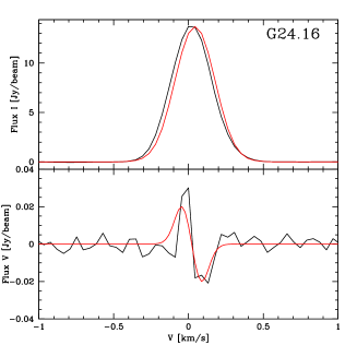
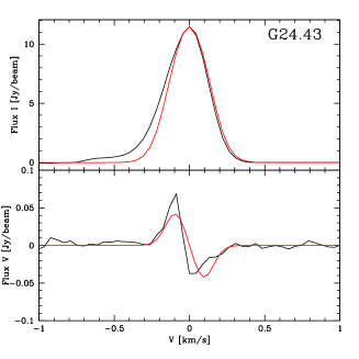
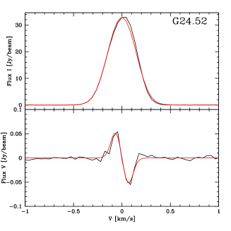
Finally, to measure the Zeeman splitting ($\Delta V_{\rm{Z}}$), we included the best estimates of $T_{\rm{b}}\Delta\Omega$ and $\Delta V_{\rm{i}}$ in the FRTM code to produce the $I$ and $V$ models used for fitting the total intensity and circularly polarized spectra of the corresponding CH₃OH maser feature (Fig. 1). Because the circularly polarized emission of CH₃OH masers is usually very weak ($<1\%$), we must take into consideration the self noise ($\sigma_{\rm{s.-n.}}$) produced by the masers (Col. 9 of Table 2; e.g., Sault sau12 (2012)) when we measure the Zeeman splitting. Therefore, we consider real a detection of circularly polarized emission only when the detected $V$ peak flux of a maser feature is both five times higher than the rms and three times larger than $\sigma_{\rm{s.-n.}}$. We know from the Zeeman effect theory that $\Delta V_{\rm{Z}}$ is related to the magnetic field strength along the line of sight ($B_{||}$) through $\Delta V_{\rm{Z}}=\alpha_{\rm{Z}}\cdot B_{||}$. However, the Landé g-factors for the CH₃OH molecule (including the 6.7 GHz maser transition) on which $\alpha_{\rm{Z}}$ depends are still unknown, and consequently, the magnetic field strength cannot yet be derived from our Zeeman-splitting measurements (e.g., Vlemmings et al. vle11 (2011)).

4 Results

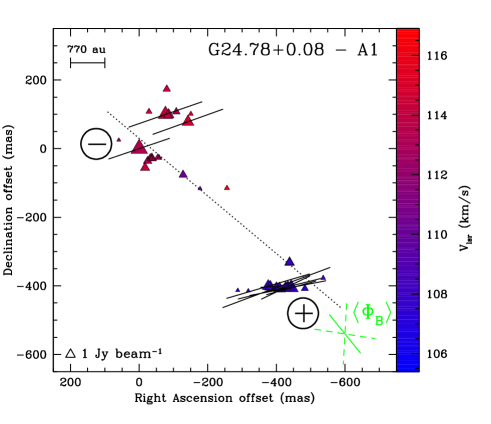
In Tables 9–15 we list all the 6.7 GHz CH₃OH maser features detected toward the seven massive SFRs observed with the EVN. The description of the maser distribution and the polarization results are reported for each source separately in Sects. 4.1–4.7. In Figs. 2–8 we show the measured linear polarization vectors as black segments and the inferred orientation of the magnetic field, which is either parallel or perpendicular to the linear polarization vectors (see Sect. 3), in green in the bottom right corner of each panel.

Figure 2: View of the CH₃OH maser features detected around the mm subcores A1 (left panel) and A2 (right panel) of G24.78+0.08. The reference position is $\alpha_{2000}=+18^{\rm{h}}36^{\rm{m}}12^{\rm{s}}\!.563$ and $\delta_{2000}=-07^{\circ}12^{\prime}10^{\prime\prime}\!\!.787$ (see Sect. 3). Triangle symbols identify CH₃OH maser features scaled logarithmically according to their peak flux density (Table 9). Maser LSR radial velocities are indicated by color (the assumed velocity of the region is $V_{\rm{lsr}}^{\rm{{}^{12}CO(1-0)}}=+111$ km s^-1, Furuya et al. fur02 (2002)). A 1 Jy beam^-1 symbol is plotted for illustration in both panels. The linear polarization vectors, scaled logarithmically according to polarization fraction $P_{\rm{l}}$, are overplotted. In the bottom right corner of both panels the corresponding error-weighted orientation of the magnetic field ($\langle\Phi_{\rm{B}}\rangle$, see Sect.5.1) is also reported, the two dashed segments indicate the uncertainty. The two arrows in the right panel indicate the direction, and not the actual position, of the red- and blueshifted lobes of the $\rm{{}^{12}CO(1-0)}$ outflow associated with G24.78+0.08-A2 ($\rm{PA_{outflow}^{{}^{12}CO}}=-40$^∘; Beltrán et al. bel11 (2011)). The dotted lines indicate the direction of the CH₃CN toroids (Beltrán et al. bel11 (2011)). The circled plus and minus symbols indicate where the magnetic field points away from and where toward the observer, respectively.

4.1 G24.78+0.08

We detected 53 CH₃OH maser features, named G24.01–G24.53 in Table 9, 33 toward core A1 and 20 toward A2. In Fig. 2 we show all the maser features associated with A1 in the left panel and those associated with A2 in the right panel. The maser distributions around the two cores are identical to those observed previously by Moscadelli et al. (mos07 (2007)), even though we detected about 40 maser features more. The peak flux density range (Col. 5 in Table 9) and the local standard of rest velocity ($V_{\rm{lsr}}$; Col. 6 in Table 9) range are similar to previous measurements.
We detected linearly polarized emission from ten CH₃OH maser features around A1 ($P_{\rm{l}}^{\rm{A1}}=0.8\%-3.5\%$) and from three maser features around A2 ($P_{\rm{l}}^{\rm{A2}}=1.0\%-1.3\%$). The adapted FRTM code was able to fit all of them but G24.38. The outputs of the code are reported in Cols. 10, 11, and 14 of Table 9. The twelve maser features for which we estimated $T_{\rm{b}}\Delta\Omega$ are unsaturated. Indeed, $T_{\rm{b}}\Delta\Omega<2.6\times 10^{9}$ K sr (or in logarithmic value $<9.4$ log K sr). For the maser features G24.23 and G24.52, both associated with A1, we have that $|\theta^{\rm{+}}-55$^∘$|<|\theta^{\rm{-}}-55$^∘$|$, that is, the magnetic field is assumed to be parallel to their linear polarization vectors as described in Sect. 3. We also measured $\Delta V_{\rm{Z}}$ for five CH₃OH maser features (Col. 13 of Table 9), only one of which is associated with A2. The circular polarization fraction ($P_{\rm{V}}$) ranges from 0.3% to 0.7% and the Zeeman splitting is $-9.7$ m s^-1$\leq\Delta V_{\rm{Z}}^{\rm{A1}}\leq+7.8$ m s^-1 around A1 and $\Delta V_{\rm{Z}}^{\rm{A2}}=(-4.0\pm 0.8)$ m s^-1 around A2 (see Fig. 1).

4.2 G25.65+1.05

Figure 3: View of the CH₃OH maser features detected around G25.65+1.05 (Table 10). Same symbols as in Fig. 2. The assumed velocity of the YSO is $V_{\rm{lsr}}^{\rm{N_{2}H^{+}-C_{2}H}}=+42.41$ km s^-1 (Sánchez-Monge et al. san13 (2013)). The two arrows indicate the direction, and not the actual position, of the red- and blueshifted lobe of the bipolar outflow ($\rm{PA_{outflow}^{\rm{SiO}}}=-15$^∘; Sánchez-Monge et al. san13 (2013)). The dashed line is the best linear fit of the CH₃OH maser features of group A ($\rm{PA_{CH_{3}OH}}=-49^{\circ}\pm 7$^∘).

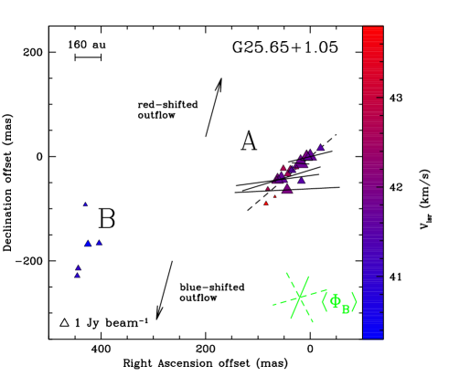
Imaging a $2^{\prime\prime}\times\leavevmode\nobreak\ 2^{\prime\prime}$ field-of-view centered on G25.02, we were able to detect a total of 23 6.7-GHz CH₃OH maser features, named G25.01–G25.23 in Table 10. The maser features can be divided into two groups (named here group A and group B) separated from each other by about 400 mas ($\sim$1300 au; see Fig. 3). The two groups are located at the origin of the bipolar outflow. Comparing our detections with the four CH₃OH maser spots detected by Walsh et al. (wal98 (1998)), which were linearly distributed southwards over $1^{\prime\prime}$, we note that only group A can be associated with one of the previous maser spots, spot B (as named by Walsh et al. wal98 (1998)). The other three CH₃OH maser spots were not detected by us, and group B was not detected by Walsh et al. (wal98 (1998)). All the maser features of group B are blueshifted with respect to the systemic velocity ($V_{\rm{lsr}}^{\rm{N_{2}H^{+}-C_{2}H}}=+42.41$ km s^-1; Sánchez-Monge et al. san13 (2013)). Even though the maser features of group A show both a linear distribution ($\rm{PA_{CH_{3}OH}}=-49^{\circ}\pm 7$^∘) and red- and blueshifted velocities, no clear velocity gradient is observed.
Five CH₃OH maser features of group A show linearly polarized emission ($P_{\rm{l}}=0.3\%-1.3\%$), and according to the output of the adapted FRTM code all of them are unsaturated (see Col. 11 of Table 10). For the maser features G25.02 and G25.06 we determined that $|\theta^{\rm{+}}-55$^∘$|<|\theta^{\rm{-}}-55$^∘$|$, that is, the magnetic field is assumed to be parallel to their linear polarization vectors. For the other maser features we found that $|\theta^{\rm{+}}-55$^∘$|>|\theta^{\rm{-}}-55$^∘$|$. We did not detect any circularly polarized maser emission toward the region ($P_{\rm{V}}<1.5\%$).

4.3 G29.86-0.04

Figure 4: View of the CH₃OH maser features detected around G29.86-0.04 (Table 11). Same symbols as in Fig. 2. The assumed velocity of the massive SFR region is $V_{\rm{lsr}}^{\rm{C^{18}O}}=+101.85$ km s^-1 (de Villiers et al. dev14 (2014)). The two arrows indicate the direction, and not the actual position, of the red- and blueshifted lobe of the bipolar outflow ($\rm{PA_{red-shifted}^{\rm{{}^{13}CO}}}\approx+6$^∘ and $\rm{PA_{blue-shifted}^{\rm{{}^{13}CO}}}\approx+60$^∘; de Villiers et al. dev14 (2014)). The dashed lines are the best linear fit to the positions of the CH₃OH maser features of group A and B ($\rm{PA_{CH_{3}OH}^{A}}=+8^{\circ}\pm 7$^∘ and $\rm{PA_{CH_{3}OH}^{B}}=-49^{\circ}\pm 5$^∘).

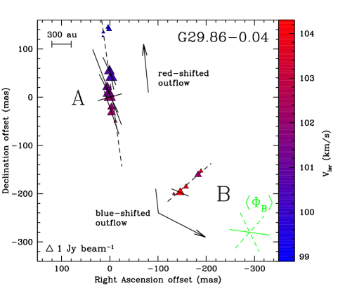
In Table 11 and Fig. 4 we report the 18 CH₃OH maser features that we detected in the region. We divided the maser features into two groups (A and B), and from a linear fit we find that the features of group A are aligned with the redshifted lobe of the outflow ($\rm{PA_{CH_{3}OH}^{A}}=+8^{\circ}\pm 7$^∘and $\rm{PA_{red-shifted}^{\rm{{}^{13}CO}}}\approx+6$^∘). The five maser features of group B are instead linearly distributed perpendicularly to the blueshifted lobe of the outflow ($\rm{PA_{CH_{3}OH}^{B}}=-49^{\circ}\pm 5$^∘and $\rm{PA_{blue-shifted}^{\rm{{}^{13}CO}}}\approx+63$^∘), even though they are spatially associated with the redshifted lobe (see Fig. B-1 of de Villiers et al. dev14 (2014)). The maser features of group A show a velocity gradient, from north (the most blueshifted velocity) to south (the most redshifted velocity), the range of which is consistent with the velocities of the quiescent emission of $\rm{{}^{13}CO}$ ($+96.5$ km s^-1$<V_{\rm{quiescent}}^{\rm{{}^{13}CO}}<+104$ km s^-1; de Villiers et al. dev14 (2014)). The velocity range of group B is also consistent with $V_{\rm{quiescent}}^{\rm{{}^{13}CO}}$.
Almost 40% of the CH₃OH maser features show linearly polarized emission ($P_{\rm{l}}=1.2\%-17\%$) and only the highest linearly polarized feature (i.e., G29.17 in Table 11) appears to have a high saturation degree ($T_{\rm{b}}\Delta\Omega=6.3\times 10^{10}$ K sr). From our analysis of the estimated $\theta$ values we determined that the magnetic field is perpendicular to all the maser features but G29.14, for which $\theta=67^{\circ\leavevmode\nobreak\ +10^{\circ}}_{-46^{\circ}}$. We measured a Zeeman splitting of $\Delta V_{\rm{Z}}=-6.6\pm 1.1$ m s^-1 toward G29.09 ($P_{\rm{V}}=0.5\%$; see Fig. 1).

4.4 G35.03+0.35

Figure 5: View of the CH₃OH maser features detected around G35.03+0.35 (Table 12). Same symbols as in Fig. 2. The assumed velocity of the massive SFR region is $V_{\rm{lsr}}=+51.5$ km s^-1 (Paron et al. par12 (2012)). The dotted line indicates the direction, and not the actual position, of the bipolar 4.5 $\mu$m emission ($\rm{PA^{4.5\,\mu m}}\approx+27^{\circ}$; Cyganowski et al. cyg09 (2009)) and the two arrows indicate the direction of the red- and blueshifted lobes of the ¹²CO-outflow (Paron et al. par12 (2012)). The dashed line is the best linear fit of the CH₃OH maser features ($\rm{PA_{CH_{3}OH}}=-26^{\circ}\pm 19$^∘).

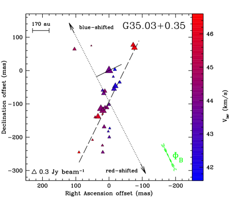
Across a bandwidth that covers a range of velocities between $-6$ km s^-1 and +94 km s^-1 , we detected 29 6.7-GHz CH₃OH maser features with velocities +41.5 km s^-1$<V_{\rm{lsr}}<$+46.7 km s^-1(see Table 12). No redshifted features were detected, as previously reported (Szymczak et al. szy00 (2000); Pandian et al. pan11 (2011)). The maser features (Fig. 5) are distributed from southeast to northwest ($\rm{PA_{CH_{3}OH}}=-26^{\circ}\pm 19$^∘) almost perpendicular to the 4.5 $\mu$m emission. In Fig. 5 we have drawn the two arrows assuming that the bipolar 4.5 $\mu$m emission also traces the ¹²CO large-scale outflow (Cyganowski et al. cyg09 (2009), Paron et al. par12 (2012)).
Because of the weak 6.7 GHz CH₃OH maser features, we were able to measure linear polarization only toward the brightest maser feature G35.19 ($P_{\rm{l}}=0.9\%$), which appears to be unsaturated. The corresponding $\theta$ angle was $+90^{\circ}\pm 24$^∘. No circularly polarized emission was detected ($P_{\rm{V}}<0.8\%$).

4.5 G37.43+1.51

Figure 6: View of the CH₃OH maser features detected around G37.43+1.51 (Table 13). Same symbols as in Fig. 2. The assumed velocity of the massive SFR region is $V_{\rm{lsr}}^{\rm{C^{18}O}}=+44.1$ km s^-1 (López-Sepulcre et al. sep10 (2010)). The two arrows indicate the direction, and not the actual position, of the red- and blueshifted lobes of the C¹⁸O-outflow ($\rm{PA_{outflow}^{\rm{C^{18}O}}}=-4$^∘; López-Sepulcre et al. sep10 (2010)). The dashed line is the best linear fit of the CH₃OH maser features ($\rm{PA_{CH_{3}OH}}=-64^{\circ}\pm 5$^∘).

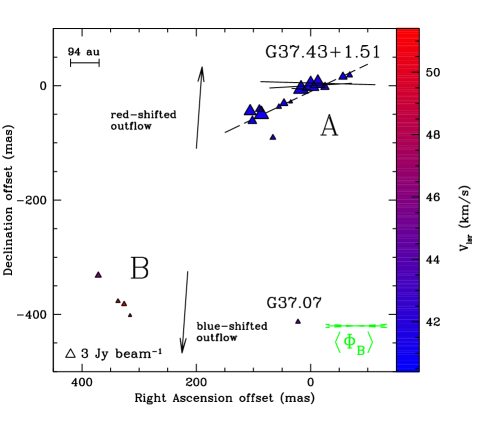
We detected two groups of CH₃OH maser features, named group A and group B in Fig. 6, separated by 300 mas ($\sim$550 au). Group A is composed of 14 maser features distributed linearly with $\rm{PA_{CH_{3}OH}}=-64^{\circ}\pm 5$^∘ with no clear velocity gradient, as already reported by Fujisawa et al. (fuj14 (2014)). The velocities of group A are consistent with the velocity range of the blueshifted lobe of the C¹⁸O-outflow (López-Sepulcre et al. sep10 (2010)). Maser features of group B were not detected before. This group, which is located southeast w.r.t. group A, show a velocity range of between 46 km s^-1 and 52 km s^-1. Furthermore, an isolated maser feature (G37.07; see Table 13) that cannot be associated with either of the two groups is located at 400 mas ($\sim$750 au) south and 300 mas ($\sim$560 au) west from groups A and B, respectively.
We detected linearly polarized emission from three CH₃OH maser features of group A ($P_{\rm{l}}=0.7\%-1.5\%$), all of which have an estimated $T_{\rm{b}}\Delta\Omega$ lower than the saturation threshold. The FRTM code estimated that the magnetic field is parallel to all the linear polarization vectors of these features, indeed $|\theta^{\rm{+}}-55$^∘$|<|\theta^{\rm{-}}-55$^∘$|$ (see Col. 14 of Table 13). No circular polarization was measured ($P_{\rm{V}}<0.2\%$).

4.6 G174.20-0.08

Figure 7: View of the CH₃OH maser features detected around the millimeter core MM1 of G174.20-0.08 (Table 14). Same symbols as in Fig. 2. The assumed velocity of the massive SFR region is $V_{\rm{lsr}}^{\rm{CH_{3}CN}}=-1.0$ km s^-1 (Zhang et al. zha07 (2007)). The two arrows indicate the direction, and not the actual position, of the red- and blueshifted lobes of the ¹²CO-outflow ($\rm{PA_{outflow}^{\rm{H_{2}O}}}=-40$^∘; Goddi et al. god11 (2011)).

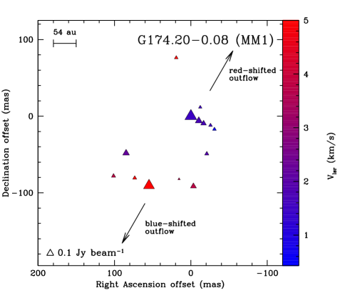
The 14 6.7-GHz CH₃OH maser features detected toward AFGL 5142 are shown in Fig. 7. No CH₃OH maser emission with a peak flux density $>0.9$ Jy beam^-1 was detected. Both the maser distribution and the velocity range of the masers agree with previous observations (e.g., Goddi et al. god11 (2011)). We were not able to detect at 5$\sigma$ either linearly polarized ($P_{\rm{l}}<0.02\%$) or circularly polarized maser emissions ($P_{\rm{V}}<0.02\%$).

4.7 G213.70-12.6

Figure 8: View of the CH₃OH maser features detected toward Star A in the massive SFR G213.70-12.6 (Mon R2-IRS3; Table 15). Same symbols as in Fig. 2. The assumed velocity of the massive SFR region is $V_{\rm{lsr}}^{\rm{{}^{13}CO(2-1)}}=+10.5$ km s^-1 (Dierickx et al. die15 (2015)). The arrows indicate the direction, and not the actual position, of the red- and blueshifted ¹³CO(2-1)-outflow powered by IRS 3 ($\rm{PA_{outflow}^{\rm{{}^{13}CO(2-1)}}}=+53$^∘; Dierickx et al. die15 (2015)). The dashed line is the best linear fit of the CH₃OH maser features ($\rm{PA_{CH_{3}OH}}=+63^{\circ}\pm 2$^∘).

We detected 20 CH₃OH maser features that are linearly distributed from northeast to southwest with $\rm{PA_{CH_{3}OH}}=+63^{\circ}\pm 2$^∘(see Fig. 8). Because the most western maser features (G213.01–G213.04 in Table 15) were previously undetected (Minier et al. min00 (2000)), the linear distribution of the maser features is now more extended (545 mas; $\sim$450 au).
Six of the CH₃OH maser features showed linearly polarized emission ($P_{\rm{l}}=3.0\%-5.0\%$), and according to the estimated $T_{\rm{b}}\Delta\Omega$ three of them are unsaturated (G213.08, G213.12, and G213.13). The FRTM code estimated $\theta$ angles greater than 55^∘ , indicating that the magnetic field is perpendicular to all the measured linear polarization vectors. Furthermore, we detected a circular polarization of 0.6% toward the brightest CH₃OH maser feature (G213.15), which implies a Zeeman splitting of $\Delta V_{\rm{Z}}=-6.6\pm 1.0$ m s^-1.

5 Discussion

Table 2: Comparison between the position angle of the magnetic field, CH₃OH maser distribution, outflows, and linear polarization angles.

(1)	(2)	(3)	(4)	(5)	(6)	(7)	(8)	(9)	(10)	(11)
Source	$\Phi_{\rm{f}}$	$\langle\chi\rangle$	$\langle\Phi_{\rm{B}}\rangle$	$\rm{PA}_{\rm{outflow}}$	$\rm{PA}_{\rm{CH_{3}OH}}$	$\rho$	$|\rm{PA}_{\rm{outflow}}-\langle\Phi_{\rm{B}}\rangle|$	$|\rm{PA}_{\rm{CH_{3}OH}}-\langle\chi\rangle|$	$|\rm{PA}_{\rm{CH_{3}OH}}-\rm{PA}_{\rm{outflow}}|$	ref.
	(∘)	(∘)	(∘)	(∘)	(∘)		(∘)	(∘)	(∘)
IRAS 20126+4104	$4$	$-70\pm 16$	$+20\pm 16$	$-65\pm 5$	$+87\pm 4$	$+0.12$	$85\pm 17$	$23\pm 17$	$28\pm 6$	(1), (2)
G24.78+0.08-A2	$17$	$-53\pm 2$	$+37\pm 2$	$-40\pm 15$	$-26\pm 19$	$-0.77$	$77\pm 15$	$79\pm 19$	$66\pm 24$	(3), (4)
G25.65+1.05	$7$	$-80\pm 8$	$-23\pm 51$	$-15\pm 15$	$-49\pm 7$	$-0.87$	$8\pm 53$	$31\pm 11$	$64\pm 17$	(3), (5)
G29.86-0.04	$17$	$+46\pm 41$	$+82\pm 56$	$+6\pm 15$	$+8\pm 7$	$+0.73$	$76\pm 58$	$38\pm 42$	$14\pm 17$	(3), (6)
G35.03+0.35	$8$	$-64\pm 5$	$+26\pm 5$	$+27\pm 15$	$-26\pm 19$	$-0.77$	$1\pm 16$	$38\pm 20$	$53\pm 24$	(3), (7), (8)
G37.43+1.51	$4$	$+90\pm 3$	$+90\pm 3$	$-4\pm 15$	$-64\pm 5$	$-0.87$	$86\pm 15$	$26\pm 6$	$60\pm 16$	(3), (9)
G174.20-0.08	$4$	$-$	$-$	$-40\pm 15$	$-63\pm 16$	$-0.45$	$-$	$-$	$23\pm 22$	(3), (10)
G213.70-12.6-IRS3	$2$	$+20\pm 5$	$-70\pm 5$	$+53\pm 15$	$+63\pm 2$	$+0.95$	$57\pm 16$	$43\pm 5$	$10\pm 15$	(3), (11)
From Paper II.
Cepheus A	$2$	$-57\pm 28$	$+30\pm 19$	$+40\pm 4$	$-79\pm 9$	$-0.34$	$10\pm 19$	$22\pm 29$	$61\pm 10$	(12)
W75N-group A	$3$	$-13\pm 9$	$+77\pm 9$	$+66\pm 15$	$+43\pm 10$	$+0.96$	$11\pm 18$	$56\pm 14$	$23\pm 18$	(12)
NGC7538-IRS1	$6$	$-30\pm 69$	$+67\pm 70$	$-40\pm 10$	$+84\pm 7$	$+0.15$	$73\pm 71$	$66\pm 69$	$56\pm 12$	(12)
W3(OH)-group II	$4$	$+21\pm 45$	$-47\pm 44$	$-$	$-59\pm 6$	$-0.84$	$-$	$80\pm 45$	$-$	(12)
W51-e2	$12$	$+33\pm 16$	$-60\pm 21$	$-50\pm 20$	$+57\pm 8$	$+0.70$	$10\pm 29$	$24\pm 18$	$73\pm 22$	(12)
IRAS18556+0138	$5$	$-2\pm 11$	$+88\pm 11$	$+58\pm 23$	$-40\pm 2$	$-0.99$	$30\pm 26$	$42\pm 11$	$82\pm 23$	(12)
W48	$7$	$+23\pm 7$	$-67\pm 7$	$-$	$+55\pm 10$	$+0.70$	$-$	$78\pm 12$	$-$	(12)
IRAS06058+2138-NIRS1	$4$	$+49\pm 47$	$-49\pm 52$	$-50\pm 15$	$+78\pm 7$	$+0.64$	$1\pm 54$	$29\pm 48$	$52\pm 17$	(12)
IRAS22272+6358A	$2$	$-80\pm 15$	$+9\pm 15$	$-40\pm 15$	$-35\pm 11$	$-0.87$	$49\pm 21$	$45\pm 19$	$5\pm 19$	(12)
S255-IR	$4$	$+36\pm 12$	$-54\pm 12$	$+75\pm 15$	$-63\pm 49$	$-0.11$	$51\pm 19$	$81\pm 51$	$42\pm 51$	(12)
S231	$4$	$+28\pm 49$	$-62\pm 49$	$-47\pm 5$	$+28\pm 8$	$+0.97$	$15\pm 49$	$0\pm 50$	$75\pm 9$	(12)
G291.27-0.70	$7$	$-32\pm 5$	$+52\pm 5$	$-$	$-77\pm 14$	$-$	$-$	$45\pm 15$	$-$	(12)
G305.21+0.21	$9$	$-51\pm 14$	$28\pm 14$	$-$	$+48\pm 23$	$-$	$-$	$81\pm 27$	$-$	(12)
G309.92+0.47	$12$	$+2\pm 56$	$-75\pm 56$	$-$	$+35\pm 5$	$-$	$-$	$33\pm 56$	$-$	(12)
G316.64-0.08	$3$	$-67\pm 36$	$+21\pm 36$	$-$	$+34\pm 29$	$-$	$-$	$79\pm 46$	$-$	(12)
G335.79+0.17	$8$	$+44\pm 28$	$-41\pm 28$	$-$	$-69\pm 25$	$-$	$-$	$67\pm 38$	$-$	(12)
G339.88-1.26	$7$	$+77\pm 24$	$-12\pm 24$	$-$	$-60\pm 17$	$-$	$-$	$43\pm 29$	$-$	(12)
G345.01+1.79	$5$	$+5\pm 39$	$-86\pm 39$	$-$	$+74\pm 4$	$-$	$-$	$69\pm 39$	$-$	(12)
NGC6334F (central)	$5$	$+77\pm 20$	$-13\pm 20$	$+30\pm 15$	$-41\pm 16$	$-$	$43\pm 25$	$62\pm 26$	$71\pm 41$	(12); (13)
NGC6334F (NW)	$5$	$-71\pm 20$	$+19\pm 20$	$+30\pm 15$	$-80\pm 38$	$-$	$11\pm 25$	$9\pm 43$	$70\pm 41$	(12); (13)

5.1 Magnetic field orientations

Linear polarization vectors may undergo a rotation when the radiation crosses a medium that is immersed in a magnetic field. This phenomenon is known as Faraday rotation. Because the polarized maser emission may be affected by two of these Faraday rotations, the internal ($\Phi_{\rm{i}}$) and the foreground Faraday rotation ($\Phi_{\rm{f}}$), we briefly determined whether their effects are negligible or not. The former, that is, $\Phi_{\rm{i}}$, can be considered negligible as explained in Papers I and II, while $\Phi_{\rm{f}}$ needs to be estimated numerically by using Eq. 3 of Paper I. We find that $\Phi_{\rm{f}}$ ranges between about 2^∘ and 17^∘, for four sources it is within the errors of the measured linear polarization angles (see Tables 9–15), and for three sources it is larger. However, $\Phi_{\rm{f}}$ is very uncertain because the errors of some parameters used to calculate it cannot be estimated. Therefore we did not correct either the $\langle\chi\rangle$ angles or the $\langle\Phi_{\rm{B}}\rangle$ angles, but we list $\Phi_{\rm{f}}$ in Col.2 of Table 6 for reader judgment.
We now discuss separately the orientation of the magnetic field in the massive SFRs toward which we detected linearly polarized CH₃OH maser emission.

G24.78+0.08. Taking into account that for G24.23 and G24.52 the magnetic field is derived to be parallel to the linear polarization vector, the error-weighted orientation of the magnetic field around A1 and A2 is $\langle\Phi_{\rm{B}}^{\rm{A1}}\rangle=+39^{\circ}\pm 42$^∘ and $\langle\Phi_{\rm{B}}^{\rm{A2}}\rangle=+37^{\circ}\pm 2$^∘, respectively. Although for G24.78+0.08 $\Phi_{\rm{f}}=17$^∘, the magnetic fields in both cores are oriented preferentially along the velocity gradient of the toroidal structures (PA${}_{\rm{A1}}=+50$^∘ and PA${}_{\rm{A2}}=+40$^∘; Beltrán et al. bel11 (2011)), and not along the CO-outflow ($\rm{PA_{outflow}^{\rm{{}^{12}CO}}}=-40$^∘; Beltrán et al. bel11 (2011)), indicating that the magnetic field is possibly located on their surfaces (see Fig. 2). Furthermore, in A1 the Zeeman-splitting measurements are spatially distributed with the negative measurement in the northern maser group and the positive measurement in the southern maser group (see left panel of Fig. 2). We recall that if $\Delta V_{\rm{Z}}>0,$ the magnetic field points away from the observer, and if $\Delta V_{\rm{Z}}<0,$ toward the observer, the magnetic field around A1 shows a counterclockwise direction that is opposite to the rotation of the toroidal structure. This is similar to what Surcis et al. (2011a ) measured in NGC7538. We also note that from our measurements the magnetic field seems to wrap the gas along the preferential southeast-northwest direction of star formation (Beltrán et al. bel11 (2011)). We measured $\Delta V_{\rm{Z}}<0$ toward A2, but in this case, because we have only one measurement, we cannot determine if the magnetic field behaves similarly to the field associated with A1. Unfortunately, we cannot discern if the magnetic field is associated directly with the two toroidal structures or with the gas that surrounds all the cores.

G25.65+1.05. We measured an error-weighted orientation of the magnetic field of $\langle\Phi_{\rm{B}}\rangle=-23^{\circ}\pm 51$^∘ by taking into account that for G25.02 and G25.06 $|\theta^{\rm{+}}-55$^∘$|<|\theta^{\rm{-}}-55$^∘$|$ (see Sect. 4.2). Therefore, the magnetic field is oriented along the SiO outflow ($\rm{PA_{outflow}^{\rm{SiO}}}=-15$^∘; Sánchez-Monge et al. san13 (2013)). For G25.02 $|\theta^{\rm{+}}-55$^∘$|$ is smaller than $|\theta^{\rm{-}}-55$^∘$|$ by only 1^∘. This indicates that the probability that the magnetic field is parallel to the linear polarization vector is not as high as to completely exclude the opposite. However, even if we consider that the magnetic field is perpendicular to the linear polarization vector of G25.02, we still have that the magnetic field ($\langle\Phi_{\rm{B}}^{\prime}\rangle=+1^{\circ}\pm 37$^∘) is preferentially oriented along the outflow. If we now compare our measurements, both $\langle\Phi_{\rm{B}}\rangle$ and $\langle\Phi_{\rm{B}}^{\prime}\rangle$, with the measurement of the magnetic field at arcsecond scale ($\rm{\Phi_{B}^{760\mu m}=+8^{\circ}\pm 16}$^∘; Vallée & Bastien val00 (2000)), we find a good agreement within the errors.

Figure 9: Left: The probability distribution function (PDF, top panel) and the cumulative distribution function (CDF, bottom panel) of the projected angle between the PA of the CH₃OH maser distribution and the linear polarization angles ($|\rm{PA}_{\rm{CH_{3}OH}}-\langle\chi\rangle|$). Right: The PDF and the CDF of the projected angle between the PA of the CH₃OH maser distribution and the outflow axes ($|\rm{PA}_{\rm{CH_{3}OH}}-\rm{PA_{\rm{outflow}}}|$). In both panels the dashed line is the CDF for random orientation of outflows and magnetic fields, i.e., all angular differences are equally likely. The results of the Kolmogorov-Smirnov test are listed in Table 8.

G29.86-0.04. Although $\Phi_{\rm{f}}=17$^∘ is estimated to be large, the magnetic field is oriented almost east-west on the plane of the sky ($\langle\Phi_{\rm{B}}\rangle=+82^{\circ}\pm 56$^∘), which is consistent with the orientation of the bent blueshifted lobe of the CO-outflow. However, because the magnetic field orientation is estimated from the polarized emission of masers that are spatially associated with the redshifted lobe of the CO-outflow, we must only compare it with the orientation of the redshifted lobe. Therefore, the magnetic field is almost perpendicular to it, suggesting that perhaps the CH₃OH masers probe a magnetic field that might be twisted around the axis of the redshifted lobe of the CO-outflow. However, because we have only one Zeeman-splitting measurement, which indicates that the magnetic field is pointing toward the observer, our interpretation is merely speculative.

G35.03+0.35. We were able to determine the magnetic field orientation on the plane of the sky from one linear polarization measurement ($\Phi_{\rm{B}}=+26^{\circ}\pm 5$^∘). The magnetic field is oriented along the 4.5 $\mu$m emission and the projection on the plane of the sky of the CO-outflow.

G37.43+1.51. The magnetic field is assumed to be parallel to all the linear polarization vectors of the 6.7 GHz CH₃OH masers measured toward group A of this massive SFR, that is, $\langle\Phi_{\rm{B}}\rangle=+90^{\circ}\pm 3$^∘. The magnetic field is thus perpendicular to the orientation on the plane of the sky of the C¹⁸O-outflow ($\rm{PA_{outflow}^{\rm{C^{18}O}}}=-4$^∘; López-Sepulcre et al. sep10 (2010)).

G213.70-12.6. The magnetic field at mas resolution shows an orientation on the plane of the sky of $\langle\Phi_{\rm{B}}\rangle=-70^{\circ}\pm 5$^∘. The magnetic field thus appears to be aligned with the linear polarization vector of Star A ($\rm{PA}^{\rm{Star\leavevmode\nobreak\ A}}_{P_{\rm{l}}}=-68^{\circ}\pm 2$^∘; Simpson et al. sim13 (2013)), which the CH₃OH masers are associated with, but it is rotated by about 90^∘ with respect to the magnetic field inferred from the polarimetric measurements at scales larger than $0^{\prime\prime}\!.2$ (Yao et al. yao97 (1997); Simpson et al. sim13 (2013)). The magnetic field probed by the masers is almost aligned with the large-scale CO-outflow detected toward IRS 6 ($\rm{PA}_{\rm{outflow}}^{\rm{CO}}\approx-45$^∘; Xu et al. xu06 (2006)), but it is almost perpendicular to the small-scale ¹³CO(2-1) outflow associated with IRS 3 ($\rm{PA}_{\rm{outflow}}^{\rm{CO}}\approx+53$^∘; Dierickx et al. die15 (2015)). Similarly to G29.86-0.04, we here speculate that the magnetic field in G213.70-12.6 might be twisted along the outflow axis.
The Zeeman splitting is measured from the circularly polarized spectra of the brightest maser G213.15 (Fig. 1). Because G213.15 is assumed to be partially saturated (see Sect. 4.7), the circular polarization might be influenced by a non-Zeeman effect due to the saturation state of the maser, that is, the rotation of the axis of symmetry for the molecular quantum states (e.g., Vlemmings vle08 (2008)). Although this effect is difficult to quantify, we are quite confident that the contribution to $P_{\rm{V}}$ of this non-Zeeman effect is not high enough to invert the $S$-shape of the $V$ spectra. Otherwise, we would have measured a much higher value of $T_{\rm{b}}\Delta\Omega$ for G213.15, which is slightly above the saturation threshold of $\rm{log}(T_{\rm{b}}\Delta\Omega)=9.4$ log(K sr). Consequently, from the sign of the Zeeman splitting, we can conclude that the magnetic field is pointing toward the observer.

5.2 Updated statistical results

At the midpoint of our project to determine if there exists any relation between the morphology of the magnetic field on a scale of tens of astronomical unit and the ejecting direction of molecular outflow from massive YSOs, we must update our first statistical results reported in Paper II by adding the new magnetic field measurements made around the sources discussed in Sect. 5.1 and around IRAS 20126+4104 (Surcis et al. sur14 (2014)). Moreover, we also added two of the southern sources observed by Dodson & Moriarty (dod12 (2012)) to our analysis: NGC6334(central) and NGC6334(NW), which were recently associated with the blueshifted lobe of a CO-outflow (Zhang et al. zha14 (2014)). Therefore we analyzed the probability distribution function (PDF) and the cumulative distribution function (CDF) of the projected angles $|\rm{PA}_{\rm{outflow}}-\langle\Phi_{\rm{B}}\rangle|$, $|\rm{PA}_{\rm{CH_{3}OH}}-\langle\chi\rangle|$, and $|\rm{PA}_{\rm{CH_{3}OH}}-\rm{PA}_{\rm{outflow}}|$; where $\rm{PA}_{\rm{outflow}}$ is the orientation of the large-scale molecular outflow on the plane of the sky, $\langle\Phi_{\rm{B}}\rangle$ is the error -weighted orientation of the magnetic field on the plane of the sky, $\rm{PA}_{\rm{CH_{3}OH}}$ is the orientation of the CH₃OH maser distribution, and $\langle\chi\rangle$ is the error-weighted value of the linear polarization angles. Note that although Surcis et al. (sur14 (2014)) determined the morphology of the magnetic field around IRAS 20126+4104 by observing the polarized emission of both 6.7 GHz CH₃OH and 22 GHz H₂O masers, we consider here only the orientation of the magnetic field estimated from the CH₃OH masers.
We list all the sources of the updated magnetic field total sample in Table 6; note that all the angles are the projection on the plane of the sky. For the statistical analysis we require the uncertainties of all the angles. While the errors of $\rm{PA}_{\rm{CH_{3}OH}}$ and $\langle\chi\rangle$ are easily determined, the uncertainties of $\rm{PA}_{\rm{outflow}}$ are unknown for all the new sources but IRAS 20126+4104. Therefore, as already done in Paper II, we considered a conservative uncertainty of $\pm 15$^∘. The uncertainties in Cols. 8 to 10 of Table 6 are equal to $\sigma_{\rm{x-y}}=\sqrt{\sigma^{2}_{\rm{x}}+\sigma^{2}_{\rm{y}}}$, where x and y are the two angles taken in consideration in each column.
In Figs. 9 and 10 we show the PDF and the CDF of $|\rm{PA}_{\rm{CH_{3}OH}}-\langle\chi\rangle|$, $|\rm{PA}_{\rm{CH_{3}OH}}-\rm{PA}_{\rm{outflow}}|$, and $|\rm{PA}_{\rm{outflow}}-\langle\Phi_{\rm{B}}\rangle|$. The results of the Kolmogorov-Smirnov (K-S) test are reported in Table 8. We note that the probability that the angles $|\rm{PA}_{\rm{CH_{3}OH}}-\langle\chi\rangle|$ are drawn from a random distribution is now $\sim$80%, which is 20% higher than what we computed in Paper II. On the other hand, the probability for the angles $|\rm{PA}_{\rm{CH_{3}OH}}-\rm{PA}_{\rm{outflow}}|$ decreases to 34%, which was 60% in Paper II. Note that if more than one maser group is detected toward an SFR region, we consider in our analysis the maser group that shows the longest linear distribution and that is clearly associated with the outflow. Even for scattered maser distribution (e.g., G174.20-0.08 MM1) we perform a linear fit.
Although the number of sources for which molecular outflows have been detected and for which the orientation of the magnetic field has been determined is now twice that of Paper II (18 vs. 9), the probability that the distribution of $|\rm{PA}_{\rm{outflow}}-\langle\Phi_{\rm{B}}\rangle|$ values are drawn from a random distribution is still 10%. This probability confirms our previous conclusion: the magnetic field close to the central YSO (10-100 au) is preferentially oriented along the outflow axis.
A more accurate statistical analysis will be presented in the last paper of the series when all the sources are observed and analyzed.

Figure 10: Probability distribution function (PDF, top panel) and the cumulative distribution function (CDF, bottom panel) of the projected angle between the magnetic field and the outflow axes ($|\rm{PA}_{\rm{outflow}}-\langle\Phi_{\rm{B}}\rangle|$). The dashed line is the CDF for random orientation of outflows and magnetic fields, i.e., all angular differences are equally likely. The results of the Kolmogorov-Smirnov test are listed in Table 8

6 Summary

Table 3: Results of the Kolmogorov-Smirnov test.

(1)	(2)	(3)	(4)	(5)
Angle	$N$	$D$	$\lambda$	$Q_{\rm{K-S}}(\lambda)$
$|\rm{PA}_{\rm{CH_{3}OH}}-\langle\chi\rangle|$	27	0.12	0.65	0.79
$|\rm{PA}_{\rm{CH_{3}OH}}-\rm{PA_{\rm{outflow}}}|$	19	0.21	0.94	0.34
$|\rm{PA}_{\rm{outflow}}-\langle\Phi_{\rm{B}}\rangle|$	18	0.28	1.22	0.10

We observed seven massive star-forming regions at 6.7 GHz in full polarization spectral mode with the EVN to detect the linearly and circularly polarized emission of CH₃OH masers. We detected linearly polarized emission toward all the sources but G174.20-0.08 (AFGL 5142) and circularly polarized emission toward three sources, G24.78+0.08, G29.86-0.04, and G213.70-12.6. By analyzing the polarized emission of the masers, we were able to estimate the orientation of the magnetic field around seven massive YSOs, considering that G24.78+0.08 hosts two centers of CH₃OH masers around each of the YSOs A1 and A2. The magnetic field is oriented along the outflows in two YSOs, it is almost perpendicular to the outflows in four YSOs, and in one YSOs (G24.78+0.08 A1) a comparison is not possible. Moreover, in G24.78+0.08 A1 and A2 the magnetic field is oriented along the toroidal structures. From the circularly polarized emission of the CH₃OH masers we measured Zeeman splitting toward G24.78+0.08 (both A1 and A2), G29.86-0.04, and G213.70-12.6.
We added all the magnetic field measurements made toward the YSOs presented in this work to the magnetic field total sample, which contains all the massive YSOs observed so far in full polarization mode at 6.7 GHz anywhere on the sky. Similarly to Paper II, we compared the projected angles between magnetic fields and outflows. We still find evidence that the magnetic field around massive YSOs are preferentially oriented along the molecular outflows. Indeed, the Kolmogorov-Smirnov test still shows a probability of 10% that our distribution of angles is drawn from a random distribution.

Acknowledgements. We wish to thank the anonymous referee for useful suggestions that have improved the paper. W.H.T.V. acknowledges support from the European Research Council through consolidator grant 614264. A.B. acknowledges support from the National Science Centre Poland through grant 2011/03/B/ST9/00627. M.G.B. acknowledges the JIVE Summer Student Programme 2013.

Appendix A Tables

In Tables 9–15 we list the parameters of all the CH₃OH maser features detected toward the seven massive star-forming regions observed with the EVN. The tables are organized as follows. The name of the feature is reported in Col. 1 and the group to which they belong in Col. 2. The positions, Cols. 3 and 4, refer to the maser feature used for self-calibration. The peak flux density, the LSR velocity ($V_{\rm{lsr}}$), and the FWHM ($\Delta v\rm{{}_{L}}$) of the total intensity spectra of the maser features are reported in Cols. 5 to 7. The peak flux density, $V_{\rm{lsr}}$, and $\Delta v\rm{{}_{L}}$ are obtained using a Gaussian fit. The mean linear polarization fraction ($P_{\rm{l}}$) and the mean linear polarization angles ($\chi$) that are measured across the spectrum are reported in Cols. 8 and 9. The best-fitting results obtained by using a model based on the radiative transfer theory of methanol masers for $\Gamma+\Gamma_{\nu}=1\leavevmode\nobreak\ \rm{s^{-1}}$ (Vlemmings et al. vle10 (2010), Surcis et al. 2011b ) are reported in Cols. 10 (the intrinsic thermal linewidth) and 11 (the emerging brightness temperature). The errors were determined by analyzing the full probability distribution function. The angle between the magnetic field and the maser propagation direction ($\theta$, Col. 14) is determined by using the observed $P_{\rm{l}}$ and the fit emerging brightness temperature. The errors for $\theta$ were also determined by analyzing the full probability distribution function. The value of $\theta$ in bold indicates that $|\theta^{\rm{+}}-55$^∘$|<|\theta^{\rm{-}}-55$^∘$|$, that is, the magnetic field is assumed to be parallel to the linear polarization vector (see Sect. 3). The circular polarization fraction ($P_{\rm{V}}$) and the Zeeman splitting ($\Delta V_{\rm{Z}}$) are listed in Cols. 12 and 13. The Zeeman splitting is determined by fitting the V Stokes spectra by using the best-fitting results ($\Delta V_{\rm{i}}$ and $T_{\rm{b}}\Delta\Omega$).

Table 4: Parameters of the 6.7 GHz CH₃OH maser features detected in G24.78+0.08.

(1)	(2)	(3)	(4)	(5)	(6)	(7)	(8)	(9)	(10)	(11)	(12)	(13)	(14)
Maser	Group	RA	Dec	Peak flux	$V_{\rm{lsr}}$	$\Delta v\rm{{}_{L}}$	$P_{\rm{l}}$	$\chi$	$\Delta V_{\rm{i}}$	$T_{\rm{b}}\Delta\Omega$	$P_{\rm{V}}$	$\Delta V_{\rm{Z}}$	$\theta$
		offset	offset	density
		(mas)	(mas)	(Jy/beam)	(km/s)	(km/s)	(%)	(∘)	(km/s)	(log K sr)	($\%$)	(m/s)	(∘)
G24.01	A2	-1542.297	746.773	$0.092\pm 0.005$	108.57	$0.25$	$-$	$-$	$-$	$-$	$-$	$-$	$-$
G24.02	A2	-1449.196	553.302	$0.222\pm 0.004$	106.59	$0.28$	$-$	$-$	$-$	$-$	$-$	$-$	$-$
G24.03	A2	-1416.923	510.347	$0.031\pm 0.004$	105.41	$0.20$	$-$	$-$	$-$	$-$	$-$	$-$	$-$
G24.04	A2	-1410.906	1117.249	$0.115\pm 0.014$	113.18	$0.47$	$-$	$-$	$-$	$-$	$-$	$-$	$-$
G24.05	A2	-1410.054	1112.544	$0.108\pm 0.006$	113.00	$0.34$	$-$	$-$	$-$	$-$	$-$	$-$	$-$
G24.06	A2	-1404.405	1082.697	$0.393\pm 0.006$	113.00	$0.25$	$-$	$-$	$-$	$-$	$-$	$-$	$-$
G24.07	A2	-1396.614	1063.488	$0.697\pm 0.019$	111.95	$0.24$	$-$	$-$	$-$	$-$	$-$	$-$	$-$
G24.08	A2	-1395.337	1044.547	$0.086\pm 0.010$	113.13	$0.35$	$-$	$-$	$-$	$-$	$-$	$-$	$-$
G24.09	A2	-1380.307	1059.353	$0.437\pm 0.014$	112.43	$0.30$	$-$	$-$	$-$	$-$	$-$	$-$	$-$
G24.10	A2	-1391.533	1035.954	$4.466\pm 0.019$	111.95	$0.27$	$1.3\pm 0.1$	$-51\pm 3$	$1.2^{+0.2}_{-0.2}$	$8.7^{+0.2}_{-0.1}$	$-$	$-$	$83^{+7}_{-21}$
G24.11	A2	-1387.531	1015.326	$0.233\pm 0.006$	111.64	$0.21$	$-$	$-$	$-$	$-$	$-$	$-$	$-$
G24.12	A2	-1383.656	1059.686	$0.524\pm 0.018$	111.95	$0.70$	$-$	$-$	$-$	$-$	$-$	$-$	$-$
G24.13	A2	-1358.919	984.020	$0.261\pm 0.006$	111.64	$0.28$	$-$	$-$	$-$	$-$	$-$	$-$	$-$
G24.14	A2	-1341.548	1037.778	$0.118\pm 0.004$	110.89	$1.68$	$-$	$-$	$-$	$-$	$-$	$-$	$-$
G24.15	A2	-1332.025	1310.781	$0.101\pm 0.006$	110.10	$0.65$	$-$	$-$	$-$	$-$	$-$	$-$	$-$
G24.16	A2	-1324.574	694.642	$13.699\pm 0.036$	110.41	$0.32$	$1.1\pm 0.1$	$-55\pm 5$	$1.7^{+0.2}_{-0.3}$	$8.6^{+0.4}_{-0.1}$	$0.3$	$-4.0\pm 0.8$	$82^{+8}_{-44}$
G24.17	A2	-1310.680	726.521	$0.234\pm 0.006$	109.58	$0.27$	$-$	$-$	$-$	$-$	$-$	$-$	$-$
G24.18	A2	-1307.118	705.516	$0.044\pm 0.005$	109.84	$0.13$	$-$	$-$	$-$	$-$	$-$	$-$	$-$
G24.19	A2	-1216.628	836.181	$0.054\pm 0.004$	110.98	$0.22$	$-$	$-$	$-$	$-$	$-$	$-$	$-$
G24.20	A2	-1155.445	997.989	$2.826\pm 0.019$	112.12	$0.37$	$1.0\pm 0.1$	$-53\pm 8$	$1.8^{+0.1}_{-0.2}$	$8.6^{+0.3}_{-0.3}$	$-$	$-$	$82^{+8}_{-36}$
G24.21	A1	-536.18	-377.044	$0.088\pm 0.004$	108.65	$0.27$	$-$	$-$	$-$	$-$	$-$	$-$	$-$
G24.22	A1	-482.635	-407.791	$0.255\pm 0.004$	107.21	$0.21$	$-$	$-$	$-$	$-$	$-$	$-$	$-$
G24.23	A1	-442.953	-405.630	$9.791\pm 0.025$	107.69	$0.35$	$1.3\pm 0.2$	$-74\pm 2$	$1.9^{+0.2}_{-0.4}$	$8.8^{+0.3}_{-0.2}$	$0.5$	$+7.8\pm 1.4$	$\mathbf{67^{+9}_{-44}}$
G24.24	A1	-438.171	-331.857	$1.029\pm 0.025$	107.78	$0.30$	$-$	$-$	$-$	$-$	$-$	$-$	$-$
G24.25	A1	-438.157	-330.956	$0.497\pm 0.019$	107.86	$1.90$	$-$	$-$	$-$	$-$	$-$	$-$	$-$
G24.26	A1	-433.147	-406.664	$5.128\pm 0.025$	107.78	$0.29$	$1.9\pm 0.3$	$-79\pm 2$	$1.4^{+0.2}_{-0.3}$	$8.9^{+0.3}_{-0.3}$	$-$	$-$	$83^{+7}_{-35}$
G24.27	A1	-426.504	-404.887	$1.564\pm 0.009$	108.30	$0.31$	$1.3\pm 0.1$	$-64\pm 4$	$1.5^{+0.2}_{-0.3}$	$8.8^{+0.2}_{-0.1}$	$-$	$-$	$83^{+7}_{-18}$
G24.28	A1	-408.963	-408.211	$2.670\pm 0.018$	108.00	$0.24$	$2.2\pm 0.4$	$-76\pm 2$	$1.2^{+0.2}_{-0.3}$	$9.0^{+0.4}_{-0.2}$	$-$	$-$	$81^{+9}_{-37}$
G24.29	A1	-399.852	-404.841	$1.058\pm 0.011$	108.22	$0.25$	$3.5\pm 0.6$	$-69\pm 3$	$1.0^{+0.3}_{-0.3}$	$9.3^{+0.3}_{-0.5}$	$-$	$-$	$87^{+3}_{-17}$
G24.30	A1	-382.197	-403.043	$2.013\pm 0.017$	108.00	$0.26$	$-$	$-$	$-$	$-$	$-$	$-$	$-$
G24.31	A1	-381.913	-402.766	$2.081\pm 0.016$	108.08	$0.27$	$0.8\pm 0.1$	$-87\pm 8$	$1.4^{+0.2}_{-0.2}$	$8.5^{+0.2}_{-0.1}$	$-$	$-$	$84^{+6}_{-40}$
G24.32	A1	-375.753	-401.033	$2.644\pm 0.017$	108.04	$0.33$	$2.2\pm 0.4$	$-74\pm 3$	$1.7^{+0.2}_{-0.3}$	$9.0^{+0.5}_{-0.4}$	$-$	$-$	$81^{+9}_{-34}$
G24.33	A1	-317.792	-414.340	$0.052\pm 0.005$	107.07	$0.29$	$-$	$-$	$-$	$-$	$-$	$-$	$-$
G24.34	A1	-287.293	-413.178	$0.059\pm 0.004$	106.90	$0.21$	$-$	$-$	$-$	$-$	$-$	$-$	$-$
G24.35	A1	-255.928	115.137	$0.092\pm 0.004$	116.91	$0.54$	$-$	$-$	$-$	$-$	$-$	$-$	$-$
G24.36	A1	-177.289	-116.315	$0.049\pm 0.004$	108.83	$0.23$	$-$	$-$	$-$	$-$	$-$	$-$	$-$
G24.37	A1	-150.438	101.504	$0.092\pm 0.004$	115.06	$0.30$	$-$	$-$	$-$	$-$	$-$	$-$	$-$
G24.38	A1	-142.022	78.130	$2.812\pm 0.006$	114.80	$0.41$	$1.8\pm 0.5$	$-70\pm 2$	$-$	$-$	$-$	$-$	$-$
G24.39	A1	-128.156	-76.137	$0.500\pm 0.019$	110.28	$0.64$	$-$	$-$	$-$	$-$	$-$	$-$	$-$
G24.40	A1	-108.358	107.273	$0.306\pm 0.022$	113.26	$0.32$	$-$	$-$	$-$	$-$	$-$	$-$	$-$
G24.41	A1	-85.948	98.951	$1.575\pm 0.010$	114.05	$0.31$	$-$	$-$	$-$	$-$	$-$	$-$	$-$
G24.42	A1	-80.442	173.600	$0.288\pm 0.016$	114.19	$0.30$	$-$	$-$	$-$	$-$	$-$	$-$	$-$
G24.43	A1	-76.652	99.772	$11.483\pm 0.016$	114.23	$0.33$	$1.9\pm 0.1$	$-71\pm 2$	$1.6^{+0.2}_{-0.3}$	$8.9^{+0.2}_{-0.1}$	$0.7$	$-9.7\pm 1.6$	$88^{+1}_{-21}$
G24.44	A1	-58.415	-26.639	$0.101\pm 0.006$	113.70	$0.43$	$-$	$-$	$-$	$-$	$-$	$-$	$-$
G24.45	A1	-54.370	-26.016	$0.175\pm 0.008$	113.09	$0.95$	$-$	$-$	$-$	$-$	$-$	$-$	$-$
G24.46	A1	-37.638	-28.224	$0.697\pm 0.012$	114.32	$0.49$	$-$	$-$	$-$	$-$	$-$	$-$	$-$
G24.47	A1	-36.900	-27.994	$0.739\pm 0.006$	113.70	$0.40$	$-$	$-$	$-$	$-$	$-$	$-$	$-$
G24.48	A1	-32.259	-24.931	$0.143\pm 0.004$	115.06	$0.25$	$-$	$-$	$-$	$-$	$-$	$-$	$-$
G24.49	A1	-28.796	108.014	$0.136\pm 0.006$	114.71	$0.27$	$-$	$-$	$-$	$-$	$-$	$-$	$-$
G24.50	A1	-24.822	-36.330	$0.541\pm 0.008$	113.09	$0.28$	$-$	$-$	$-$	$-$	$-$	$-$	$-$
G24.51	A1	-17.499	-56.006	$0.829\pm 0.008$	114.41	$0.31$	$-$	$-$	$-$	$-$	$-$	$-$	$-$
G24.52	A1	0	0	$32.970\pm 0.032$	113.40	$1.72$	$1.5\pm 0.4$	$-71\pm 2$	$1.8^{+0.2}_{-0.4}$	$8.8^{+0.5}_{-0.3}$	$0.3$	$-4.6\pm 0.7$	$\mathbf{73^{+2}_{-40}}$
G24.53	A1	59.167	24.964	$0.047\pm 0.005$	112.78	$0.25$	$-$	$-$	$-$	$-$	$-$	$-$	$-$

Table 5: Parameters of the 6.7 GHz CH₃OH maser features detected in G25.65+1.05.

(1)	(2)	(3)	(4)	(5)	(6)	(7)	(8)	(9)	(10)	(11)	(12)	(13)	(14)
Maser	Group	RA	Dec	Peak flux	$V_{\rm{lsr}}$	$\Delta v\rm{{}_{L}}$	$P_{\rm{l}}$	$\chi$	$\Delta V_{\rm{i}}$	$T_{\rm{b}}\Delta\Omega$	$P_{\rm{V}}$	$\Delta V_{\rm{Z}}$	$\theta$
		offset	offset	density
		(mas)	(mas)	(Jy/beam)	(km/s)	(km/s)	(%)	(∘)	(km/s)	(log K sr)	($\%$)	(m/s)	(∘)
G25.01	A	-19.690	15.911	$0.338\pm 0.014$	41.56	$0.11$	$-$	$-$	$-$	$-$	$-$	$-$	$-$
G25.02	A	0	0	$6.924\pm 0.124$	41.78	$0.31$	$0.4\pm 0.2$	$-76\pm 11$	$1.6^{+0.1}_{-0.2}$	$8.2^{+0.7}_{-1.6}$	$-$	$-$	$\mathbf{72^{+12}_{-45}}$
G25.03	A	6.886	-0.382	$3.860\pm 0.126$	42.00	$0.17$	$-$	$-$	$-$	$-$	$-$	$-$	$-$
G25.04	A	7.170	-0.828	$4.023\pm 0.108$	42.04	$0.17$	$-$	$-$	$-$	$-$	$-$	$-$	$-$
G25.05	A	16.873	-46.883	$0.311\pm 0.012$	41.52	$0.11$	$-$	$-$	$-$	$-$	$-$	$-$	$-$
G25.06	A	18.324	-13.035	$24.318\pm 0.142$	41.82	$0.21$	$0.3\pm 0.2$	$86\pm 29$	$1.1^{+0.1}_{-0.1}$	$8.1^{+1.3}_{-1.2}$	$-$	$-$	$\mathbf{59^{+5}_{-53}}$
G25.07	A	25.865	-21.118	$0.045\pm 0.004$	42.66	$0.21$	$-$	$-$	$-$	$-$	$-$	$-$	$-$
G25.08	A	34.771	-26.409	$0.448\pm 0.012$	41.52	$0.12$	$-$	$-$	$-$	$-$	$-$	$-$	$-$
G25.09	A	37.787	-23.865	$0.127\pm 0.003$	42.57	$0.22$	$-$	$-$	$-$	$-$	$-$	$-$	$-$
G25.10	A	42.823	-33.508	$0.213\pm 0.004$	42.66	$0.19$	$-$	$-$	$-$	$-$	$-$	$-$	$-$
G25.11	A	43.876	-64.026	$2.455\pm 0.108$	42.04	$0.23$	$1.3\pm 0.8$	$-87\pm 21$	$<0.5$	$8.7^{+0.2}_{-2.1}$	$-$	$-$	$90^{+59}_{-59}$
G25.12	A	51.103	-23.075	$0.126\pm 0.003$	42.75	$0.24$	$-$	$-$	$-$	$-$	$-$	$-$	$-$
G25.13	A	55.030	-42.839	$6.113\pm 0.124$	41.78	$0.19$	$0.8\pm 0.3$	$-73\pm 10$	$0.9^{+0.2}_{-0.1}$	$8.5^{+0.8}_{-1.3}$	$-$	$-$	$77^{+13}_{-37}$
G25.14	A	62.143	-44.819	$3.748\pm 0.108$	42.04	$0.20$	$0.9\pm 0.2$	$-82\pm 15$	$1.0^{+0.1}_{-0.2}$	$8.5^{+1.2}_{-0.8}$	$-$	$-$	$75^{+15}_{-37}$
G25.15	A	63.480	-41.443	$0.031\pm 0.002$	42.97	$0.21$	$-$	$-$	$-$	$-$	$-$	$-$	$-$
G25.16	A	67.236	-76.904	$0.016\pm 0.002$	43.76	$0.21$	$-$	$-$	$-$	$-$	$-$	$-$	$-$
G25.17	A	80.809	-62.267	$0.041\pm 0.003$	42.70	$0.17$	$-$	$-$	$-$	$-$	$-$	$-$	$-$
G25.18	A	84.252	-90.500	$0.043\pm 0.002$	43.80	$0.22$	$-$	$-$	$-$	$-$	$-$	$-$	$-$
G25.19	B	402.507	-166.119	$0.104\pm 0.003$	40.64	$0.27$	$-$	$-$	$-$	$-$	$-$	$-$	$-$
G25.20	B	423.904	-168.041	$0.237\pm 0.003$	40.38	$0.29$	$-$	$-$	$-$	$-$	$-$	$-$	$-$
G25.21	B	428.827	-92.293	$0.038\pm 0.003$	40.73	$0.23$	$-$	$-$	$-$	$-$	$-$	$-$	$-$
G25.22	B	442.399	-214.329	$0.106\pm 0.003$	41.03	$0.25$	$-$	$-$	$-$	$-$	$-$	$-$	$-$
G25.23	B	444.249	-228.867	$0.094\pm 0.003$	40.99	$0.24$	$-$	$-$	$-$	$-$	$-$	$-$	$-$

Table 6: Parameters of the 6.7 GHz CH₃OH maser features detected in G29.86-0.04.

(1)	(2)	(3)	(4)	(5)	(6)	(7)	(8)	(9)	(10)	(11)	(12)	(13)	(14)
Maser	Group	RA	Dec	Peak flux	$V_{\rm{lsr}}$	$\Delta v\rm{{}_{L}}$	$P_{\rm{l}}$	$\chi$	$\Delta V_{\rm{i}}$	$T_{\rm{b}}\Delta\Omega$	$P_{\rm{V}}$	$\Delta V_{\rm{Z}}$	$\theta$
		offset	offset	density
		(mas)	(mas)	(Jy/beam)	(km/s)	(km/s)	(%)	(∘)	(km/s)	(log K sr)	($\%$)	(m/s)	(∘)
G29.01	B	-188.953	-153.172	$0.150\pm 0.003$	103.68	$0.24$	$-$	$-$	$-$	$-$	$-$	$-$	$-$
G29.02	B	-183.009	-160.760	$0.971\pm 0.015$	102.05	$0.29$	$-$	$-$	$-$	$-$	$-$	$-$	$-$
G29.03	B	-157.861	-185.738	$0.275\pm 0.003$	103.85	$0.32$	$-$	$-$	$-$	$-$	$-$	$-$	$-$
G29.04	B	-145.858	-197.453	$2.423\pm 0.004$	104.29	$0.92$	$1.24\pm 0.03$	$67\pm 3$	$<0.5$	$8.9^{+0.1}_{-0.1}$	$-$	$-$	$79^{+8}_{-9}$
G29.05	B	-132.541	-200.275	$0.053\pm 0.003$	103.06	$0.41$	$-$	$-$	$-$	$-$	$-$	$-$	$-$
G29.06	A	-11.774	-50.191	$0.080\pm 0.003$	102.49	$0.24$	$-$	$-$	$-$	$-$	$-$	$-$	$-$
G29.07	A	-3.715	-32.043	$3.047\pm 0.006$	102.23	$0.20$	$3.9\pm 0.5$	$19\pm 2$	$0.9^{+0.2}_{-0.2}$	$9.3^{+0.3}_{-0.2}$	$-$	$-$	$83^{+7}_{-11}$
G29.08	A	-3.315	-20.612	$1.593\pm 0.016$	102.01	$0.18$	$-$	$-$	$-$	$-$	$-$	$-$	$-$
G29.09	A	-3.258	41.101	$19.262\pm 0.018$	100.39	$0.32$	$1.6\pm 0.3$	$11\pm 2$	$1.8^{+0.1}_{-0.2}$	$8.6^{+1.2}_{-0.1}$	$0.5$	$-6.6\pm 1.1$	$74^{+15}_{-37}$
G29.10	A	0	0	$32.456\pm 0.015$	101.88	$0.35$	$1.6\pm 0.5$	$-74\pm 1$	$1.8^{+0.1}_{-0.3}$	$8.9^{+0.4}_{-0.7}$	$-$	$-$	$73^{+17}_{-34}$
G29.11	A	0.343	58.858	$0.182\pm 0.003$	99.95	$1.69$	$-$	$-$	$-$	$-$	$-$	$-$	$-$
G29.12	A	0.857	54.225	$9.863\pm 0.009$	100.82	$0.43$	$2.1\pm 0.3$	$25\pm 8$	$<0.5$	$9.0^{+0.1}_{-0.3}$	$-$	$-$	$90^{+16}_{-16}$
G29.13	A	1.429	141.063	$0.293\pm 0.003$	99.77	$0.36$	$-$	$-$	$-$	$-$	$-$	$-$	$-$
G29.14	A	2.286	7.941	$24.431\pm 0.022$	101.48	$0.25$	$3.4\pm 2.0$	$26\pm 1$	$1.2^{+0.3}_{-0.3}$	$9.2^{+0.4}_{-0.9}$	$-$	$-$	$\mathbf{67^{+10}_{-46}}$
G29.15	A	3.372	145.423	$0.196\pm 0.003$	98.89	$0.23$	$-$	$-$	$-$	$-$	$-$	$-$	$-$
G29.16	A	5.430	20.873	$5.179\pm 0.018$	101.26	$0.23$	$17.0\pm 2.0$	$21\pm 2$	$<0.5$	$10.8^{+0.3}_{-0.3}$	$-$	$-$	$90^{+6}_{-6}$
G29.17	A	13.431	135.044	$0.083\pm 0.003$	99.03	$3.71$	$-$	$-$	$-$	$-$	$-$	$-$	$-$
G29.18	A	14.460	126.231	$0.099\pm 0.003$	99.11	$0.44$	$-$	$-$	$-$	$-$	$-$	$-$	$-$

Table 7: Parameters of the 6.7 GHz CH₃OH maser features detected in G35.03+0.35.

(1)	(2)	(3)	(4)	(5)	(6)	(7)	(8)	(9)	(10)	(11)	(12)	(13)	(14)
Maser	Group	RA	Dec	Peak flux	$V_{\rm{lsr}}$	$\Delta v\rm{{}_{L}}$	$P_{\rm{l}}$	$\chi$	$\Delta V_{\rm{i}}$	$T_{\rm{b}}\Delta\Omega$	$P_{\rm{V}}$	$\Delta V_{\rm{Z}}$	$\theta$
		offset	offset	density
		(mas)	(mas)	(Jy/beam)	(km/s)	(km/s)	(%)	(∘)	(km/s)	(log K sr)	($\%$)	(m/s)	(∘)
G35.01		78.111	64.224	$0.112\pm 0.005$	44.88	$0.24$	$-$	$-$	$-$	$-$	$-$	$-$	$-$
G35.02		67.948	-245.222	$0.061\pm 0.006$	46.63	$0.22$	$-$	$-$	$-$	$-$	$-$	$-$	$-$
G35.03		40.077	74.663	$0.026\pm 0.005$	45.10	$0.23$	$-$	$-$	$-$	$-$	$-$	$-$	$-$
G35.04		37.305	-208.235	$0.042\pm 0.007$	45.84	$0.31$	$-$	$-$	$-$	$-$	$-$	$-$	$-$
G35.05		31.409	-140.110	$0.065\pm 0.005$	45.62	$0.32$	$-$	$-$	$-$	$-$	$-$	$-$	$-$
G35.06		25.080	-138.308	$0.530\pm 0.007$	45.89	$0.38$	$-$	$-$	$-$	$-$	$-$	$-$	$-$
G35.07		18.546	-114.414	$1.164\pm 0.011$	44.26	$0.16$	$-$	$-$	$-$	$-$	$-$	$-$	$-$
G35.08		14.840	-224.552	$0.055\pm 0.008$	44.62	$0.41$	$-$	$-$	$-$	$-$	$-$	$-$	$-$
G35.09		14.658	-130.545	$0.035\pm 0.007$	45.93	$0.30$	$-$	$-$	$-$	$-$	$-$	$-$	$-$
G35.10		14.657	-59.593	$0.087\pm 0.004$	42.99	$0.16$	$-$	$-$	$-$	$-$	$-$	$-$	$-$
G35.11		14.070	-244.907	$0.099\pm 0.009$	44.09	$0.11$	$-$	$-$	$-$	$-$	$-$	$-$	$-$
G35.12		13.540	-120.426	$1.062\pm 0.013$	44.48	$0.20$	$-$	$-$	$-$	$-$	$-$	$-$	$-$
G35.13		12.015	-68.813	$0.226\pm 0.010$	43.89	$0.46$	$-$	$-$	$-$	$-$	$-$	$-$	$-$
G35.14		11.052	-169.041	$0.157\pm 0.010$	44.22	$0.15$	$-$	$-$	$-$	$-$	$-$	$-$	$-$
G35.15		9.444	-61.880	$0.182\pm 0.012$	44.48	$0.17$	$-$	$-$	$-$	$-$	$-$	$-$	$-$
G35.16		9.048	-109.791	$0.088\pm 0.009$	44.18	$0.24$	$-$	$-$	$-$	$-$	$-$	$-$	$-$
G35.17		4.780	-111.321	$0.197\pm 0.011$	44.31	$0.20$	$-$	$-$	$-$	$-$	$-$	$-$	$-$
G35.18		1.635	-182.730	$0.047\pm 0.004$	42.60	$0.25$	$-$	$-$	$-$	$-$	$-$	$-$	$-$
G35.19		0	0	$2.252\pm 0.010$	43.87	$0.46$	$0.9\pm 0.1$	$-64\pm 5$	$2.6^{+0.2}_{-0.3}$	$8.5^{+0.3}_{-0.2}$	$-$	$-$	$90^{+24}_{-24}$
G35.20		-0.201	-102.259	$0.084\pm 0.005$	43.47	$1.12$	$-$	$-$	$-$	$-$	$-$	$-$	$-$
G35.21		-0.576	-199.854	$0.087\pm 0.006$	43.34	$0.20$	$-$	$-$	$-$	$-$	$-$	$-$	$-$
G35.22		-1.651	-173.355	$0.052\pm 0.006$	42.16	$0.24$	$-$	$-$	$-$	$-$	$-$	$-$	$-$
G35.23		-9.665	-18.393	$0.051\pm 0.005$	42.38	$0.47$	$-$	$-$	$-$	$-$	$-$	$-$	$-$
G35.24		-11.233	-55.342	$0.370\pm 0.005$	42.55	$0.26$	$-$	$-$	$-$	$-$	$-$	$-$	$-$
G35.25		-13.312	2.804	$0.108\pm 0.006$	41.59	$0.28$	$-$	$-$	$-$	$-$	$-$	$-$	$-$
G35.26		-14.343	-46.606	$0.510\pm 0.007$	42.20	$0.21$	$-$	$-$	$-$	$-$	$-$	$-$	$-$
G35.27		-24.309	-35.076	$0.087\pm 0.004$	42.07	$0.25$	$-$	$-$	$-$	$-$	$-$	$-$	$-$
G35.28		-54.673	76.618	$0.284\pm 0.006$	46.15	$0.44$	$-$	$-$	$-$	$-$	$-$	$-$	$-$
G35.29		-57.559	68.207	$0.598\pm 0.006$	46.33	$0.38$	$-$	$-$	$-$	$-$	$-$	$-$	$-$

Table 8: Parameters of the 6.7 GHz CH₃OH maser features detected in G37.43+1.51.

(1)	(2)	(3)	(4)	(5)	(6)	(7)	(8)	(9)	(10)	(11)	(12)	(13)	(14)
Maser	Group	RA	Dec	Peak flux	$V_{\rm{lsr}}$	$\Delta v\rm{{}_{L}}$	$P_{\rm{l}}$	$\chi$	$\Delta V_{\rm{i}}$	$T_{\rm{b}}\Delta\Omega$	$P_{\rm{V}}$	$\Delta V_{\rm{Z}}$	$\theta$
		offset	offset	density
		(mas)	(mas)	(Jy/beam)	(km/s)	(km/s)	(%)	(∘)	(km/s)	(log K sr)	($\%$)	(m/s)	(∘)
G37.01	A	-68.621	18.314	$0.147\pm 0.004$	40.65	$0.21$	$-$	$-$	$-$	$-$	$-$	$-$	$-$
G37.02	A	-56.601	15.614	$0.522\pm 0.006$	40.79	$0.20$	$-$	$-$	$-$	$-$	$-$	$-$	$-$
G37.03	A	-25.050	-2.205	$0.525\pm 0.004$	42.23	$0.21$	$-$	$-$	$-$	$-$	$-$	$-$	$-$
G37.04	A	-12.561	4.368	$17.807\pm 0.064$	41.58	$0.23$	$1.5\pm 0.4$	$89\pm 18$	$1.2^{+0.2}_{-0.3}$	$8.8^{+1.5}_{-0.9}$	$-$	$-$	$\mathbf{71^{+5}_{-48}}$
G37.05	A	0	0	$44.137\pm 0.056$	41.36	$0.23$	$1.1\pm 1.0$	$-87\pm 15$	$1.3^{+0.1}_{-0.2}$	$8.7^{+0.8}_{-2.3}$	$-$	$-$	$\mathbf{61^{+9}_{-49}}$
G37.06	A	16.738	-5.684	$17.809\pm 0.097$	41.09	$0.17$	$0.7\pm 1.1$	$87\pm 14$	$0.9^{+0.1}_{-0.1}$	$8.5^{+0.7}_{-2.1}$	$-$	$-$	$\mathbf{60^{+5}_{-54}}$
G37.07	-	22.127	-412.994	$0.071\pm 0.003$	44.60	$0.21$	$-$	$-$	$-$	$-$	$-$	$-$	$-$
G37.08	A	34.773	-28.278	$0.133\pm 0.003$	40.43	$0.20$	$-$	$-$	$-$	$-$	$-$	$-$	$-$
G37.09	A	46.621	-30.720	$0.417\pm 0.004$	40.70	$0.27$	$-$	$-$	$-$	$-$	$-$	$-$	$-$
G37.10	A	55.475	-36.919	$0.096\pm 0.004$	42.14	$0.16$	$-$	$-$	$-$	$-$	$-$	$-$	$-$
G37.11	A	65.854	-90.763	$0.125\pm 0.009$	41.88	$0.27$	$-$	$-$	$-$	$-$	$-$	$-$	$-$
G37.12	A	86.156	-50.171	$13.038\pm 0.103$	41.14	$0.24$	$-$	$-$	$-$	$-$	$-$	$-$	$-$
G37.13	A	89.663	-40.821	$0.379\pm 0.005$	41.97	$0.17$	$-$	$-$	$-$	$-$	$-$	$-$	$-$
G37.14	A	101.995	-61.619	$0.597\pm 0.019$	40.92	$0.13$	$-$	$-$	$-$	$-$	$-$	$-$	$-$
G37.15	A	105.916	-44.788	$3.430\pm 0.072$	41.44	$0.20$	$-$	$-$	$-$	$-$	$-$	$-$	$-$
G37.16	B	315.938	-401.817	$0.032\pm 0.003$	49.87	$0.35$	$-$	$-$	$-$	$-$	$-$	$-$	$-$
G37.17	B	326.346	-381.825	$0.079\pm 0.002$	51.41	$0.42$	$-$	$-$	$-$	$-$	$-$	$-$	$-$
G37.18	B	336.867	-376.862	$0.057\pm 0.002$	50.14	$0.29$	$-$	$-$	$-$	$-$	$-$	$-$	$-$
G37.19	B	371.484	-331.863	$0.166\pm 0.004$	46.05	$0.25$	$-$	$-$	$-$	$-$	$-$	$-$	$-$

Table 9: Parameters of the 6.7 GHz CH₃OH maser features detected in G174.20-0.08.

(1)	(2)	(3)	(4)	(5)	(6)	(7)	(8)	(9)	(10)	(11)	(12)	(13)	(14)
Maser	Group	RA	Dec	Peak flux	$V_{\rm{lsr}}$	$\Delta v\rm{{}_{L}}$	$P_{\rm{l}}$	$\chi$	$\Delta V_{\rm{i}}$	$T_{\rm{b}}\Delta\Omega$	$P_{\rm{V}}$	$\Delta V_{\rm{Z}}$	$\theta$
		offset	offset	density
		(mas)	(mas)	(Jy/beam)	(km/s)	(km/s)	(%)	(∘)	(km/s)	(log K sr)	($\%$)	(m/s)	(∘)
G174.01		-30.813	-17.113	$0.047\pm 0.005$	0.43	$0.30$	$-$	$-$	$-$	$-$	$-$	$-$	$-$
G174.02		-25.677	-11.940	$0.047\pm 0.007$	1.49	$0.13$	$-$	$-$	$-$	$-$	$-$	$-$	$-$
G174.03		-20.827	-49.076	$0.057\pm 0.005$	1.88	$0.31$	$-$	$-$	$-$	$-$	$-$	$-$	$-$
G174.04		-16.548	-9.541	$0.095\pm 0.008$	1.66	$0.21$	$-$	$-$	$-$	$-$	$-$	$-$	$-$
G174.05		-12.220	11.673	$0.043\pm 0.006$	1.53	$0.17$	$-$	$-$	$-$	$-$	$-$	$-$	$-$
G174.06		-10.271	-6.065	$0.159\pm 0.007$	1.71	$0.17$	$-$	$-$	$-$	$-$	$-$	$-$	$-$
G174.07		-3.329	-91.538	$0.105\pm 0.005$	3.72	$0.34$	$-$	$-$	$-$	$-$	$-$	$-$	$-$
G174.08		0	0	$0.853\pm 0.006$	1.53	$0.24$	$-$	$-$	$-$	$-$	$-$	$-$	$-$
G174.09		15.454	-82.115	$0.029\pm 0.005$	3.72	$0.22$	$-$	$-$	$-$	$-$	$-$	$-$	$-$
G174.10		19.115	76.355	$0.046\pm 0.009$	5.04	$0.28$	$-$	$-$	$-$	$-$	$-$	$-$	$-$
G174.11		54.778	-90.572	$0.617\pm 0.010$	5.00	$0.29$	$-$	$-$	$-$	$-$	$-$	$-$	$-$
G174.12		73.560	-80.715	$0.054\pm 0.010$	5.00	$0.28$	$-$	$-$	$-$	$-$	$-$	$-$	$-$
G174.13		84.734	-48.252	$0.135\pm 0.005$	2.19	$0.19$	$-$	$-$	$-$	$-$	$-$	$-$	$-$
G174.14		101.234	-78.148	$0.058\pm 0.005$	3.77	$0.20$	$-$	$-$	$-$	$-$	$-$	$-$	$-$

Table 10: Parameters of the 6.7 GHz CH₃OH maser features detected in G213.70-12.6 (Mon R2–IRS 3/Star A).

(1)	(2)	(3)	(4)	(5)	(6)	(7)	(8)	(9)	(10)	(11)	(12)	(13)	(14)
Maser	Group	RA	Dec	Peak flux	$V_{\rm{lsr}}$	$\Delta v\rm{{}_{L}}$	$P_{\rm{l}}$	$\chi$	$\Delta V_{\rm{i}}$	$T_{\rm{b}}\Delta\Omega$	$P_{\rm{V}}$	$\Delta V_{\rm{Z}}$	$\theta$
		offset	offset	density
		(mas)	(mas)	(Jy/beam)	(km/s)	(km/s)	(%)	(∘)	(km/s)	(log K sr)	($\%$)	(m/s)	(∘)
G213.01		-444.918	-209.568	$0.111\pm 0.006$	10.11	0.17	$-$	$-$	$-$	$-$	$-$	$-$	$-$
G213.02		-436.616	-206.261	$0.098\pm 0.005$	10.07	0.33	$-$	$-$	$-$	$-$	$-$	$-$	$-$
G213.03		-334.883	-188.515	$0.105\pm 0.005$	9.98	0.15	$-$	$-$	$-$	$-$	$-$	$-$	$-$
G213.04		-304.061	-187.214	$0.469\pm 0.005$	9.94	0.18	$-$	$-$	$-$	$-$	$-$	$-$	$-$
G213.05		-130.791	-79.498	$3.650\pm 0.015$	10.99	0.21	$3.0\pm 0.4$	$17\pm 2$	$1.1^{+0.2}_{-0.3}$	$9.2^{+0.4}_{-0.1}$	$-$	$-$	$77^{+13}_{-37}$
G213.06		-124.479	-70.560	$0.570\pm 0.015$	10.99	0.19	$-$	$-$	$-$	$-$	$-$	$-$	$-$
G213.07		-112.196	-83.591	$1.139\pm 0.015$	10.99	0.21	$-$	$-$	$-$	$-$	$-$	$-$	$-$
G213.08		-72.276	-71.392	$49.360\pm 0.06$	10.68	0.24	$5.0\pm 1.4$	$51\pm 49$	$1.1^{+0.2}_{-0.4}$	$9.6^{+0.5}_{-0.5}$	$-$	$-$	$71^{+19}_{-27}$
G213.09		-67.784	-97.511	$1.750\pm 0.050$	10.77	0.18	$-$	$-$	$-$	$-$	$-$	$-$	$-$
G213.10		-53.624	-42.149	$0.562\pm 0.006$	11.21	0.21	$-$	$-$	$-$	$-$	$-$	$-$	$-$
G213.11		-49.189	-52.086	$0.055\pm 0.004$	12.04	0.59	$-$	$-$	$-$	$-$	$-$	$-$	$-$
G213.12		-35.882	-0.412	$2.470\pm 0.060$	10.68	0.26	$3.1\pm 0.3$	$15\pm 6$	$<0.5$	$9.2^{+0.1}_{-0.1}$	$-$	$-$	$90^{+13}_{-13}$
G213.13		-33.721	-2.464	$5.355\pm 0.007$	11.39	0.26	$4.3\pm 0.3$	$23\pm 3$	$1.1^{+0.5}_{-0.4}$	$9.4^{+0.3}_{-0.1}$	$-$	$-$	$85^{+6}_{-21}$
G213.14		-11.601	-12.871	$0.173\pm 0.005$	12.31	0.33	$-$	$-$	$-$	$-$	$-$	$-$	$-$
G213.15		0	0	$91.580\pm 0.050$	12.57	0.24	$4.6\pm 0.4$	$16\pm 7$	$1.1^{+0.1}_{-0.4}$	$9.5^{+0.3}_{-0.1}$	$0.6$	$-6.6\pm 1.0$	$82^{+8}_{-17}$
G213.16		9.269	-39.421	$0.461\pm 0.011$	13.23	0.25	$-$	$-$	$-$	$-$	$-$	$-$	$-$
G213.17		16.377	13.481	$4.603\pm 0.008$	13.40	0.25	$3.4\pm 0.3$	$21\pm 2$	$1.1^{+0.2}_{-0.3}$	$9.5^{+0.3}_{-0.1}$	$-$	$-$	$72^{+18}_{-29}$
G213.18		22.860	25.299	$0.139\pm 0.004$	13.71	0.27	$-$	$-$	$-$	$-$	$-$	$-$	$-$
G213.19		28.376	33.211	$1.702\pm 0.009$	13.36	0.26	$-$	$-$	$-$	$-$	$-$	$-$	$-$
G213.20		35.086	49.870	$0.054\pm 0.004$	12.00	0.67	$-$	$-$	$-$	$-$	$-$	$-$	$-$

References

- (1) Argon, A.L., Reid, M.J., & Menten, K.M. 2000, ApJS, 129, 159
- (2) Beltrán, M.T., Cesaroni, R., Neri, R. et al., 2004, ApJ, 601, L187
- (3) Beltrán, M.T., Cesaroni, R., Neri, R. et al., 2005, A&A, 435, 901
- (4) Beltrán, M.T., Cesaroni, R., Codella, C. et al., 2006, Nature, 443, 427
- (5) Beltrán, M.T., Cesaroni, R., Zhang, Q. et al. 2011, A&A, 532, A91
- (6) Breen, S.L. & Ellingsen, S.P. 2011, MNRAS, 416, 178
- (7) Carpenter, J.M., Meyer, M.R., Dougados, M.R. et al. 1997, AJ, 114, 198
- (8) Caswell, J.L., Gardner, F.F., Norris, R.P. et al. 1993, MNRAS, 260, 425
- (9) Caswell, J.L., Vaile, R.A., Ellingsen, S.P. et al. 1995, MNRAS, 272, 96
- (10) Caswell, J.L., Green, J.A., & Phillips, C.J. 2013, MNRAS, 431, 1180
- (11) Cesaroni, R., Codella, C., Furuya, R.S. et al. 2003, A&A, 401, 227
- (12) Chapman, N.L., Davidson, J.A., Goldsmith, P.F. et al. 2013, ApJ, 770, 151
- (13) Codella, C., Testi, L. & Cesaroni, R. 1997, A&A, 325, 282
- (14) Codella, C., Beltrán, M.T., Cesaroni, R. et al. 2013, A&A, 550, A81
- (15) Cyganowski, C.J., Brogan, C.L., Hunter, T.R. et al. 2009, ApJ, 702, 1615
- (16) Cyganowski, C.J., Brogan, C.L., Hunter, T.R. et al. 2011, ApJ, 743, 56
- (17) Curran, R.L. & Chrysostomou, A. 2007, MNRAS, 382, 699
- (18) de Villiers, H.M., Chrysostomou, A., Thompson, M.A. et al. 2014, MNRAS, 444, 566
- (19) Dierickx, M., Jiménez-Serra, I., Rivilla, V.M. et al. 2015, arXiv:1503.05230v1
- (20) Dodson, R. & Moriarty, C.D. 2012, MNRAS, 421, 2395
- (21) Forster, J.R. & Caswell, J.L. 1999, A&AS, 137, 43
- (22) Fujisawa, K., Sugiyama, K., Motogi, K. et al. 2014, PASJ, 66, 31
- (23) Furuya, R.S., Cesaroni, R., Codella, C. et al. 2002, A&A, 390, L1
- (24) Galván-Madrid, R., Rodríguez, L.F., Ho, P.T.P. et al. 2008, ApJ, 674, L33
- (25) Goddi, C., Moscadelli, L., Sanna, A. et al. 2007, A&A, 461, 1027
- (26) Goddi, C., Moscadelli, L, Sanna, A. 2011, A&A, 535, L8
- (27) Goldreich, P., Keeley, D.A., & Kwan, J.Y., 1973, ApJ, 179, 111
- (28) Henning, Th., Chini, R. & Pfau, W. 1992, A&A, 263, 285
- (29) Herbst, W. & Racine, R. 1976, AJ, 81, 840
- (30) Hill, T., Burton, M.G., Minier, V. et al. 2005, MNRAS, 363, 405
- (31) Hill, T., Thompson, M.A., Burton, M.G. et al. 2006, MNRAS, 368, 1223
- (32) Howard, E.M., Pipher, J.L., & Forrest, W.J. 1994, ApJ, 425, 707
- (33) Hull, C.L.H., Plambeck, R.L., Bolatto, A.D. et al. 2013, ApJ, 768, 159
- (34) Hunter, T.R., Testi, L., Taylor, G.B. et al. 1995, A&A, 302, 249
- (35) Hunter, T.R., Churchwell, E., Watson, C. et al. 2000, ApJ, 119, 2711
- (36) Keimpema, A., Kettenis, M.M., Pogrebenko, S.V., et al. 2015, Experimental Astronomy, arXiv:1502.00467
- (37) Kurtz, S., Churchwell, E., & Wood, D.O.S. 1994, ApJSS, 91, 659
- (38) López-Sepulcre, A., Cesaroni, R. & Walmsley, C.M. 2010, A&A, 517, A66
- (39) McKee, C.F. & Tan, J.C. 2003, ApJ, 585, 850
- (40) McKee, C. F. & Ostriker E.C. 2007, ARA&A, 45, 565
- (41) Minier, V., Booth, R.S., & Conway, J.E. 2000, A&A, 362, 1093
- (42) Molinari, A., Brand, J., Cesaroni, R. et al. 1996, A&A, 308, 573
- (43) Moscadelli, L., Goddi, C., Cesaroni, R. et al. 2007, A&A, 472, 867
- (44) Moscadelli, L., Cesaroni, R., Riojia, M.J., et al. 2011, A&A, 526, A66
- (45) Myers, A.T., McKee, C.F., Cunningham, A.J. et al. 2013, ApJ, 766, 97
- (46) Palau, A., Fuente, A., Girart, J.M. et al. 2011, ApJ, 743, L32
- (47) Pandian, J.D., Momjian, E., Xu, Y. et al. 2011, ApJ, 730, 55
- (48) Paron, S., Ortega, M.E., Petriella, A. et al. 2012, MNRAS, 419, 2206
- (49) Pestalozzi, M.R., Minier, V., & Booth, R.S. 2005, A&A, 432, 737
- (50) Peters, T., Banerjee, R., Klessen, R.S. et al. 2011, ApJ, 729, 72
- (51) Preibisch, T., Balega, Y.Y., Schertl, D. et al. 2002, A&A, 392, 945
- (52) Sánchez-Monge, A., López-Sepulcre, A., Cesaroni, R. et al. 2013, A&A, 557, A94
- (53) Sault, R.J. 2012, EVLA Memo 159
- (54) Schutte, A.J., van der Walt, D.J., Gaylard, M.J. et al. 1993, MNRAS, 261, 783
- (55) Seifried, D., Pudritz, R.E., Banerjee, R. et al. 2012, MNRAS, 422, 347
- (56) Shepherd, D.S. & Churchwell, E. 1996, ApJ, 457, 267
- (57) Simpson, J.P., Whitney, B.A., Hines, D.C. et al. 2013, MNRAS, 435, 3419
- (58) Snell, R.L., Huang, Y.-L., Dickman, R.L. et al. 1988, ApJ, 325, 853
- (59) Surcis, G., Vlemmings, W.H.T., Dodson, R. et al. 2009, A&A, 506, 757
- (60) Surcis, G., Vlemmings, W.H.T., Torres, R.M. et al. 2011a, A&A, 533, A47
- (61) Surcis, G., Vlemmings, W.H.T., Curiel, S. et al. 2011b, A&A, 527, A48
- (62) Surcis, G., Vlemmings, W.H.T., van Langevelde, H.J. et al. 2012, A&A, 541, A47, Paper I
- (63) Surcis, G., Vlemmings, W.H.T., van Langevelde, H.J. et al. 2013, A&A, 556, A73, Paper II
- (64) Surcis, G., Vlemmings, W.H.T., van Langevelde, H.J. et al. 2014, A&A, 563, A30
- (65) Szymczak, M., Hrynek, G., & Kus, A.J., 2000, A&AS, 143, 269
- (66) Torrelles, J.M., Gómez, J.F., Anglada, G. et al. 1992, ApJ, 392, 616
- (67) Vallée, J.P. & Bastien, P. 2000, ApJ, 530, 806
- (68) Varricatt, W.P., Davis, C.J., Ramsay, S. et al. 2010, MNRAS, 404, 661
- (69) Vlemmings, W.H.T. 2008, A&A, 484, 773
- (70) Vlemmings, W.H.T., Surcis, G., Torstensson, K.J.E. et al. 2010, MNRAS, 404, 134
- (71) Vlemmings, W.H.T., Torres, R.M., & Dodson, R. 2011, A&A, 529, A95
- (72) Walsh, A.J., Burton, M.G., Hyland, A.R. et al. 1998, MNRAS, 301, 640
- (73) Walsh, A.J., MacDonald, G.H., Alvey, N.D.S et al. 2003, A&A, 410, 597
- (74) Wardle, J.F.C. & Kronberg, P.P. 1974, ApJ, 194, 249
- (75) Wu, Y.W., Sato, M., Reid, M.J. et al. 2014, A&A, 566, A17
- (76) Xu, Y., Shen, Z.-Q., Yang, J. et al. 2006, ApJ, 132, 20
- (77) Yao, Y., Hirata, N., Ischii, M. et al. 1997, ApJ, 490, 281
- (78) Zavagno, A., Deharveng, L., Nadeau, D. et al. 2002, A&A, 394,225
- (79) Zhang, Q., Hunter, T.R., Beuther, H. et al. 2007, ApJ, 658, 1152
- (80) Zhang, Q., Qiu, K., Girart, J.M. et al. 2014, ApJ, 792, 116