Tensor Numerical Methods in Quantum Chemistry:
from Hartree-Fock Energy to Excited States

Abstract

We resume the recent successes of the grid-based tensor numerical methods and discuss their prospects in real-space electronic structure calculations. These methods, based on the low-rank representation of the multidimensional functions and integral operators, first appeared as an accurate tensor calculus for the 3D Hartree potential using 1D complexity operations, and have evolved to entirely grid-based tensor-structured 3D Hartree-Fock eigenvalue solver. It benefits from tensor calculation of the core Hamiltonian and two-electron integrals (TEI) in $O(n\log n)$ complexity using the rank-structured approximation of basis functions, electron densities and convolution integral operators all represented on 3D $n\times n\times n$ Cartesian grids. The algorithm for calculating TEI tensor in a form of the Cholesky decomposition is based on multiple factorizations using algebraic 1D “density fitting“ scheme , which yield an almost irreducible number of product basis functions involved in the $3$D convolution integrals, depending on a threshold $\varepsilon>0$. The basis functions are not restricted to separable Gaussians, since the analytical integration is substituted by high-precision tensor-structured numerical quadratures. The tensor approaches to post-Hartree-Fock calculations for the MP2 energy correction and for the Bethe-Salpeter excited states, based on using low-rank factorizations and the reduced basis method, were recently introduced. Another direction is related to the recent attempts to develop a tensor-based Hartree-Fock numerical scheme for finite lattice-structured systems, where one of the numerical challenges is the summation of electrostatic potentials of a large number of nuclei. The 3D grid-based tensor method for calculation of a potential sum on a $L\times L\times L$ lattice manifests the linear in $L$ computational work, $O(L)$, instead of the usual $O(L^{3}\log L)$ scaling by the Ewald-type approaches. The accuracy of the order of atomic radii, $h\sim 10^{-4}\AA{}$, for the grid representation of electrostatic potentials is achieved due to low cost of using $1$D operations on large 3D grids.

Key words: Electronic structure calculations, two-electron integrals, multidimensional integrals, tensor decompositions, quantized tensor approximation, low-rank Cholesky factorization, reduced higher order SVD, Hartree-Fock equation, excited states, lattice potential sums.

AMS Subject Classification: 65F30, 65F50, 65N35, 65F10

1 Introduction

The problems of numerical modeling the many-particle interactions in large molecular systems, lattice structured metallic clusters and crystals, proteins and nanomaterials are the most challenging tasks in modern computational physics and chemistry. The traditional approaches for these multidimensional problems are restricted to the concepts which have well recognized limitations for computations with higher accuracy and for larger non-periodic molecular systems, as well as for efficient calculation of excited states. Recent advances in numerical analysis for multidimensional problems and significant achievements in high performance computing suggest new creative approaches to these problems.

The Hartree-Fock (HF) equation governed by the 3D integral-differential operator [66, 28] is one of the basic models for ab initio calculation of the ground state energy of molecular systems. It is a strongly nonlinear eigenvalue problem (EVP) in a sense, that one should solve the equation in a self-consistent way when the integral part of the governing operator depends on the solution itself. Multiple strong singularities in the electron density of a molecule due to nuclear cusps impose strong requirements on the accuracy of calculations.

Commonly used numerical methods for solution of the Hartree-Fock equation are based on the analytical computation of the arising two-electron integrals (convolution type integrals in $\mathbb{R}^{3}$) in the problem adapted naturally separable Gaussian-type bases [1], by using erf-function expansions. This rigorous approach resulted in a number of efficient implementations which are widely used in computational quantum chemistry. The success of the analytical integration methods stems from the big amount of precomputed information based on the physical insight including the construction of problem adapted atomic orbitals basis sets and elaborate nonlinear optimization for calculation of density fitting basis. The known limitations of this approach appear due to a strong dependence of the numerical efficiency on the size and quality of the chosen Gaussian basis sets, that might be crucial for larger molecular clusters and heavier atoms.

The intention to replace or assist the analytical calculations for the Hartree-Fock problem by a data-sparse grid-based numerical schemes has a long history. First success was the grid-based numerical method for the diatomic molecules in [65], though this approach was not feasible to compact (3D) molecules. The wavelet multiresolution schemes [12] capable for the accurate representation of nuclear cusps, have been applied to electronic structure simulations since the seminal papers [27, 62], and recently this approach was further advanced due to achievements in the high performance supercomputing [62, 8, 19, 17]. However, due to extensive computational resources, the entirely wavelet-based or sparse-grid approaches [23, 73] are limited so far only to rather small atomic systems with few electrons [2]. Tensor hyper-contraction decompositions in density fitting schemes have been analyzed in [31, 58].

The newly developed tensor-structured numerical methods, both the name and the concept, appeared during the work on the grid-based tensor approach to the solution of the 3D Hartree-Fock problem [37, 38, 41]. The central point is the representation of $d$-variate functions and integral/differential operators on large $n^{\otimes d}$ grids and their approximation in the low-rank tensor formats, which allows numerical calculations in $O(dn)$ complexity instead of $O(n^{d})$ by conventional methods.

In this paper we summarize the main benefits of the tensor numerical methods in electronic structure calculations, and discuss further prospects of this approach in several directions, such as

• algebraic directional density fitting and tensor factorization of the two-electron integrals and their use in the Hartree-Fock calculations;

• tensor decompositions in the MP2 energy correction, and in calculation of excited states based on the Bethe-Salpeter equation;

• fast tensor summation of electrostatic potentials on large 3D lattice for efficient calculation of the Fock matrix in the case of lattice-structured systems;

• fast calculation of the interaction energy of the long-range potentials on large 3D lattices.

Notice that basic rank-structured tensor formats such as the canonical (PARAFAC) and Tucker tensor decompositions have been since long used in the computer science for the quantitative analysis of correlations in the experimental multidimensional data arrays in data processing and chemometrics, see [49] and references therein. In 2006 the exceptional properties of the Tucker decomposition for the discretized multidimensional functions have been revealed in [35, 37], where it was proven that for a class of function-related tensors the approximation error of the Tucker decomposition decays exponentially with respect to the Tucker rank. This gives the opportunity to represent the discretized multidimensional functions and integral (convolution) operators in an algebraically separable form and thus reduce the numerical treatment of the multidimensional transforms to 1D operations. It was shown that the number of vectors in such a representation depends only logarithmically on the size of the $d$-dimensional grid, $O(n^{d})$, used for discretization of multivariate functions.

The above results have led to the idea to calculate the Hartree potential and the Coulomb and exchange operators by numerical quadratures [38] using Gaussian-type basis functions discretized on 3D Cartesian grids and the fast tensor-product convolution [34]. In this way, the efficient low-rank canonical tensor representation to the Newton kernel was an essential contribution [7]. To reduce the initial rank of the electron density, that is quadratically proportional to the number of GTO basis functions, the canonical-to-Tucker tensor transform was invented [38, 37], which made computations for large tensor grids and extended molecules tractable (even in Matlab).

The initial version of tensor-structured algorithms for solving Hartree-Fock equation employed the 3D grid-based calculation of the Coulomb and exchange integral operators ”on-the-fly”, thus avoiding precomputation and storage of the TEI tensor[39, 41]. In particular, it was justified that tensor calculus allows to reduce the 3D convolution integrals to combinations of 1D convolutions, and 1D Hadamard and scalar products. Besides, these results promoted spreading of the tensor-structured methods in the community of numerical analysis [21, 36, 26], and further development of the tree-tensor formats like tensor-train [56] and hierarchical Tucker representations [25].

Further development of tensor methods in electronic structure calculations was due to the fast algorithm for the grid-based computation of the TEI tensor [43] in $O(N_{b}^{3})$ storage in the number of basis functions $N_{b}$. The fourth order TEI tensor is calculated in a form of the Cholesky factorization by using the algebraic 1D ”density fitting“ scheme, which applies to the product basis functions. Imposing the low-rank tensor representation of the product basis functions and the Newton convolving kernel all discretized on $n\times n\times n$ Cartesian grid, the 3D integral transforms are calculated in $O(n\log n)$ complexity. Given the factorized TEI, the update of the Column and exchange parts in the Fock matrix reduces to the cheap algebraic operations. Other steps are tensor calculation of the core Hamiltonian and the efficient MP2 energy correction scheme [44], which all together gave rise to the black-box Hartree-Fock solver [45].

Due to the grid representation of basis functions basis sets are now not restricted to Gaussian-type orbitals and allowed to be any well-separable function defined on a grid. The tensor-based Hartree-Fock solver is competitive in computational time and accuracy with the standard packages based on analytical calculation of integrals. High accuracy is attained owing to easy calculations on large 3D grids up to $n^{3}=10^{18}$, so that the resolution with mesh size $h$ of the order of atomic radii, $10^{-4}\AA{}$, is possible.

Motivated by tensor decompositions in the MP2 scheme, the new approach for calculation of the excited states in the framework of the Bethe-Salpeter equation was recently introduced [6], that employs the reduced basis method in combination with low-rank tensor approximations.

Further developments of the tensor methods in multi-particle simulations are focused on the large lattice structures in a box and nearly periodic systems, for which the tensor approach may reduce computational costs dramatically [47]. One of the challenging problems in the numerical treatment of the crystalline-type molecular clusters is summation of a large number of electrostatic potentials distributed on a finite (non-periodic) lattice. The novel grid-based method for summation of the long-range potentials in the canonical and Tucker formats [46, 48] works on $L\times L\times L$ lattices with the computational cost $O(L)$ instead of $O(L^{3}\log L)$ by the traditional Ewald-type methods [18]. The required precision is guaranteed by employing large 3D Cartesian grids for representation of potentials. The method remains efficient for lattices with non-rectangular geometries and in the presence of multiple defects [48, 47].

The rest of the paper is organized as follows. In Section 2, we overview the basic tensor formats and show why the orthogonal Tucker tensor decomposition, originating from computer science and data processing, became useful for the treatment of the multidimensional functions and operators in numerical analysis. In particular, §2.3 and §2.4 discuss the matrix product states (tensor train) formats and the novel quantics tensor approximation method, respectively, while §2.5 addresses the basic tensor-structured multilinear algebra operations. Section 3 describes tensor calculus of the multidimensional convolution transform on examples of the Hartree potential (§3.1) and the TEI tensor (§3.2), and recalls the main building blocks in the tensor-based black-box Hartree-Fock solver. Section 4 shows benefits of the tensor approach in MP2 calculations and in calculation of the lowest part of the excitation energies in the framework of the Bethe-Salpeter equation. Section 5 describes the benefits of tensor methods in applications to lattice-type molecular systems. In particular, we present fast tensor method for the summation of the long-range interaction potentials on a 3D lattice by using the assembled vectors of their canonical and Tucker tensor representations. The important application of this approach to calculation of interaction energy of the Coulombic potentials on a lattice with sub-linear cost in the lattice size is described in detail. Appendix discusses some computational details on the Canonical-to-Tucker tensor transform, the Galerkin discretization scheme for the nonlinear Hartree-Fock equation, and the basics of the low-rank canonical tensor representation for the Newton kernel.

2 Rank-structured tensor representations of discretized functions and operators

In this section we discuss shortly why the rank-structured tensors, which were traditionally used in experimental data processing, appears to be useful for the separable representation of multivariate functions and operators represented on tensor product grids. The canonical and Tucker tensor decompositions have been since long used in the computer science community for the quantitative analysis of correlations in the experimental multidimensional data arrays in chemometrics and data processing, with rather weak requirements on the accuracy, see [63, 49] and references therein. In the recent decade the class of matrix product states type tensor formats became popular in the simulations of quantum spin systems and quantum molecular dynamics. We refer to [49, 61, 36] for recent literature surveys on commonly used tensor formats.

2.1 Canonical and Tucker tensor formats

We consider a tensor of order $d$, as a real multidimensional array ${\bf A}=[a_{i_{1},...,i_{d}}]\in\mathbb{R}^{n_{1}\times\ldots\times n_{d}}$ numbered by a $d$-tuple index set, with multi-index notation ${\bf i}=(i_{1},...,i_{d})$, $i_{\ell}\in\{1,...,n_{\ell}\},\ell=1,...,d$. It is an element of the linear vector space $\mathbb{R}^{n_{1}\times\ldots\times n_{d}}$ equipped with the Euclidean scalar product,

$$\left\langle{\bf A},{\bf B}\right\rangle=\sum_{i_{1}=1}^{n_{1}}\cdots\sum_{i_{d}=1}^{n_{d}}a_{i_{1},...,i_{d}}b_{i_{1},...,i_{d}}.$$

Euclidean vectors and matrices are the special case of $d$th order tensors. For a general tensor, the required storage scales exponentially in the dimension, $n_{1}n_{2}\cdots n_{d}$, (the so-called ”curse of dimensionality“). To get rid of exponential scaling in the dimension, one can apply the rank-structured separable representations of multidimensional tensors. The simplest separable element is given by rank-$1$ canonical tensor,

$${\bf U}={\bf u}^{(1)}\otimes...\otimes{\bf u}^{(d)}\in\mathbb{R}^{n_{1}\times\ldots\times n_{d}},$$

with entries

$$u_{i_{1},\ldots,i_{d}}=u^{(1)}_{i_{1}}\cdot\cdot\cdot u^{(d)}_{i_{d}},$$

requiring only $n_{1}+...+n_{d}$ numbers to store it.

A tensor in the $R$-term canonical format is defined by

$${\bf U}={\sum}_{k=1}^{R}c_{k}{\bf u}_{k}^{(1)}\otimes\ldots\otimes{\bf u}_{k}^{(d)},\quad c_{k}\in\mathbb{R},$$ (2.1)

where ${\bf u}_{k}^{(\ell)}\in\mathbb{R}^{n_{\ell}}$ are normalized vectors, and $R$ is called the canonical rank of a tensor. It is convenient to introduce the so-called side matrices $U^{(\ell)}=[{\bf u}_{1}^{(\ell)}\ldots{\bf u}_{R}^{(\ell)}]\in\mathbb{R}^{n_{\ell}\times R}$, $\ell=1,2,3$, obtained by concatenation of the canonical vectors ${\bf u}_{k}^{(\ell)}$, $k=1,\ldots R$. Now the storage cost is bounded by $dRn$. For $d\geq 3$ computation of the canonical rank of a tensor ${\bf U}$, i.e. the minimal number $R$ in representation (2.1) and the respective decomposition, is an $N$-$P$ hard problem. In the case $d=2$ the representation (2.1) is merely a rank-$R$ matrix.

We say that a tensor ${\bf V}$ is represented in the rank-$\bf r$ orthogonal Tucker format with the rank parameter ${\bf r}=(r_{1},...,r_{d})$, if

$${\bf V}=\sum\limits_{\nu_{1}=1}^{r_{1}}\ldots\sum\limits^{r_{d}}_{{\nu_{d}}=1}\beta_{\nu_{1},\ldots,\nu_{d}}\,{\bf v}^{(1)}_{\nu_{1}}\otimes\ldots\otimes{\bf v}^{(d)}_{\nu_{d}},\quad\ell=1,\ldots,d,$$ (2.2)

where $\{{\bf v}^{(\ell)}_{\nu_{\ell}}\in\mathbb{R}^{n_{\ell}}\}$ represents the set of orthonormal vectors, and $\boldsymbol{\beta}=[\beta_{\nu_{1},...,\nu_{d}}]\in\mathbb{R}^{r_{1}\times\cdots\times r_{d}}$ is the Tucker core tensor. The storage cost for the Tucker tensor is bounded by $drn+r^{d}$, $r=\max r_{\ell}$. In the case $d=2$, the orthogonal Tucker decomposition is equivalent to the singular value decomposition (SVD) of a rectangular matrix. Figure 2.1 visualizes the canonical and Tucker tensors in the case $d=3$.

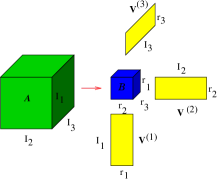
Figure 2.1: Visualizing the canonical and Tucker tensors for $d=3$.

Canonical tensor decomposition leads to an ill-posed problem and, up to our best knowledge, there are no robust algebraic algorithms for the canonical approximation of an arbitrary tensor. For some classes of analytic functions, the explicit low-rank approximation can be constructed in analytic form by using $sinc$-quadrature approximation to the Laplace transform. The robust methods for Tucker decomposition are based on the orthogonal projections using the higher order singular value decomposition[15] (HOSVD) that is the generalization of the singular value decomposition (SVD) of matrices.

The rank-structured decomposition (approximation) of multidimensional tensors provides means for the separation of variables in the discretized representation of multivariate functions and operators, and thus the possibility to substitute multidimensional algebraic transforms by univariate operations. Notice that in the computer science community these possibilities were restricted to moderate-dimensional tensors of small mode size (with rather large rank parameters) obtained from the experimental data sets.

2.2 Tucker decomposition for function related tensors. Canonical-to-Tucker approximation

In 2006 it was first verified numerically, see in [37], that the rank of the (fixed accuracy) Tucker approximation to some function related tensors depends only logarithmically on the size of the discretization grid. For a given continuous function $f:\Omega\to\mathbb{R}$, $\Omega:=\prod^{d}_{\ell=1}[a_{\ell},b_{\ell}]\subset\mathbb{R}^{3}$, we introduced the function related $3$rd order tensor, obtained by Galerkin discretization in a volume box using $n\times n\times n$ 3D Cartesian grid. In particular, the low-rank tensor approximations were calculated for functions of the Slater type $f(x)=\exp(-\alpha\|x\|)$, Newton kernel $f(x)=\frac{1}{\|x\|}$, Yukawa potential $f(x)=\frac{e^{-\alpha\|x\|}}{\|x\|}$, and the Helmholtz potential $f(x)=\frac{\cos{\alpha\|x\|}}{\|x\|}$, $x\in\mathbb{R}^{3}$.

Numerical tests demonstrated that the error of the rank-${\bf r}$ (with ${\bf r}=(r,r,r)$) Tucker approximation applied to these third order tensors decays exponentially with respect to the Tucker rank $r$. Moreover, for fixed approximation error, the Tucker rank $r$ scales as $O(\log n)$ for above mentioned functions [34].

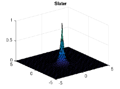
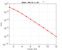
Figure 2.2: The Tucker approximation error in the Frobenius norm vs. the Tucker rank $r$ for a single Slater function.

This application revealed a number of properties of the Tucker format which were not known before. In particular, it was showed that for tensors resulting from the discretization of physically relevant multidimensional functions on the tensor grids one can find algebraically a reduced subspace in each mode of the original tensor, thus approximating the function by separated variables using a tensor product of a relatively small number of vectors.

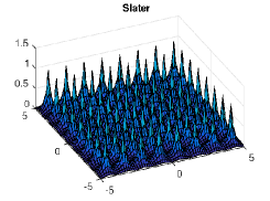
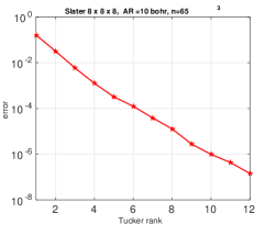
Figure 2.3: The Tucker approximation error in the Frobenius norm vs. the Tucker rank $r$ for a sum of Slater potentials over the cubic $8\times 8\times 8$ lattice (right).

Figures 2.2 and 2.3 (right) show the exponential convergence of the Tucker tensor approximation in the Tucker rank $r$ of the Slater function in the relative Frobenius norm, $E_{FN}=\frac{\|A-A_{r}\|}{\|A\|}$. Figures demonstrate that the exponential decay of approximation error is nearly the same for both a single potential and for a sum of the same potentials distributed in nodes of a cubic lattice. This property of the Tucker decomposition will be further gainfully applied to the fast lattice summation of interaction potentials.

Motivated by these observations, we invented the canonical-to-Tucker (C2T) decomposition for function related tensors [37], based on the reduced higher order singular value decomposition (RHOSVD) (Theorem 2.5, [38]). The canonical-to-Tucker algorithm (see Appendix) combined with the Tucker-to-canonical transform serves for reducing the ranks of canonical tensors with large $R$.

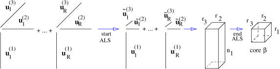
Figure 2.4: Part of the canonical-to-Tucker decomposition algorithm for mode $\ell=1$.

Figure 2.4 in its ALS part shows the algorithmic step for $\ell=1$, which is repeated for every mode $\ell=1,2,3$ (see Appendix). The computational work for the multigrid tensor decomposition C2T algorithm introduced in [38] exhibits linear complexity scaling with respect to all input parameters, $O(Rnr)$.

The multigrid Tucker decomposition algorithm applied to full format tensors [38] leads to the complexity scaling $O(n^{3})$, whereas its standard version (commonly used HOSVD algorithm in computer science) scales as $O(n^{4})$, becoming intractable even for moderate sizes of tensors.

We conclude by notice that the optimized Tucker and canonical tensor approximations can be computed by the alternating least square (ALS) iteration with initial guess obtained by HOSVD/RHOSVD approximations.

2.3 Matrix Product States/Tensor Train format

The product-type representation of $d$th order tensors, which is called in the physical literature as the matrix product states (MPS) decomposition (or more generally, tensor network states models), was introduced and successfully applied in DMRG quantum computations [72, 68, 61], and, independently, in quantum molecular dynamics as the multilayer (ML) MCTDH methods [70, 53]. MPS type representations reduce the storage complexity to $O(dr^{2}N)$, where $r$ is the maximal rank parameter.

In the recent years the various versions of the MPS-type tensor approximations were discussed and further investigated in mathematical literature including the hierarchical dimension splitting [35], the tensor train (TT) [56, 13], the quantics-TT (QTT) [33], as well as the hierarchical Tucker representation [25], which belongs to the class of tensor network states model.

The TT format is the particular form of MPS type factorization in the case of open boundary conditions. For a given rank parameter ${\bf r}=(r_{0},...,r_{d})$, the rank-${\bf r}$ TT format contains all elements ${\bf A}=[a_{i_{1},...,i_{d}}]\in\mathbb{R}^{n_{1}\times...\times n_{d}}$, which can be represented as the contracted products of $3$-tensors, that in the index notation takes a form,

$$a_{i_{1},...,i_{d}}=\sum\limits_{\alpha_{1}=1}^{r_{1}}\cdots\sum\limits_{\alpha_{d}=1}^{r_{d}}{\bf a}^{(1)}_{\alpha_{1}}(i_{1}){\bf a}^{(2)}_{\alpha_{1},\alpha_{2}}(i_{2})\cdot\cdot\cdot{\bf a}^{(d)}_{\alpha_{d-1}}(i_{d})\equiv{A}^{(1)}({i_{1}}){A}^{(2)}({i_{2}})\ldots{A}^{(d)}({i_{d}}),$$

specified by the set of column vectors, ${\bf a}^{(\ell)}_{\alpha_{\ell},\alpha_{\ell+1}}\in\mathbb{R}^{n_{\ell}}$, ($\ell=1,...,d$), or equivalently by the vector-valued $r_{\ell}\times r_{\ell+1}$ matrices, ${A}^{(\ell)}=[{\bf a}^{(\ell)}_{\alpha_{\ell},\alpha_{\ell+1}}]$, (i.e., $3$-tensors), cf. (2.2). The latter representation is written in the matrix product form, explaining the notion MPS, where ${A}^{(\ell)}(i_{\ell})$ is $r_{\ell-1}\times r_{\ell}$ matrix.

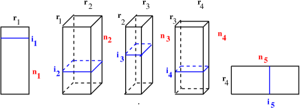
Figure 2.5: Visualizing $5$th-order MPS/TT tensor.

Figure 2.5 illustrates the TT representation of a $5$th-order tensor, where each particular entry is factorized as a product of five matrices, $a_{i_{1},i_{2},...,i_{5}}={A}^{(1)}({i_{1}}){A}^{(2)}({i_{2}})\ldots{A}^{(5)}({i_{5}})$, where, for example, ${A}^{(2)}({i_{2}})\in\mathbb{R}^{r_{1}\times r_{2}}$.

The rank-structured tensor formats like canonical, Tucker and MPS/TT-type decompositions also apply to matrices. For example, the $d$-dimensional FFT matrix over $N^{\otimes d}$ grid can be implemented on the rank-$k$ tensor with the linear-logarithmic cost $O(dkN\log_{2}N)$, due to the rank-$1$ factorized representation

$${\cal F}_{N}^{(d)}=(F_{N}^{(1)}\otimes I...\otimes I)(I\otimes F_{N}^{(2)}...\otimes I)...(I\otimes I...\otimes F_{N}^{(d)})\equiv F_{N}^{(1)}\otimes...\otimes F_{N}^{(d)},$$

where $F_{N}^{(\ell)}\in\mathbb{R}^{N\times N}$ represents the univariate FFT matrix along mode $\ell$.

2.4 Quantics tensor approximation of functional vectors

In the case of large mode size, the asymptotic storage cost for a class of function related $N$-$d$ tensors can be reduced to $O(d\log N)$ by using quantics-TT (QTT) tensor approximation method [33]. The QTT-type approximation of an $N$-vector with $N=2^{L}$, $L\in\mathbb{N}$, is defined as the tensor decomposition (approximation) in the canonical, TT or more general formats applied to a tensor obtained by the dyadic folding (reshaping) of the target vector to an $L$-dimensional $2\times...\times 2$ data array (tensor) that is thought as an element of the $L$-dimensional quantized tensor space.

In the vector case, i.e. for $d=1$, a vector ${\bf x}=[x_{i}]\in\mathbb{R}^{{N}},$ with $N=2^{L}$, is reshaped to its quantics (quantized) image in $\bigotimes_{j=1}^{L}\mathbb{R}^{2},$ by dyadic folding,

$$\mathcal{F}_{2,L}:{\bf x}\to{\bf Y}=[y_{\bf j}]\in{\bigotimes}_{j=1}^{L}\mathbb{R}^{2},\quad{\bf j}=(j_{1},...,j_{L}),\;\,j_{\nu}\in\{1,2\},$$

where for fixed $i$, we have $y_{\bf j}:=x_{i}$, with $j_{\nu}=j_{\nu}(i)=C_{\nu-1}$ ($\nu=1,...,L$) being defined via binary coding, i.e. the coefficients $C_{\nu-1}\in\{0,1\}$ are found from the binary representation of $i-1$,

$$i-1=C_{0}+C_{1}2^{1}+\cdots+C_{L-1}2^{L-1}\equiv\sum\limits_{\nu=1}^{L}(j_{\nu}-1)2^{\nu-1}.$$

Next figure visualizes the QTT approximation process.

Suppose that the quantics image for an $N$-vector, i.e. an element of $L$-dimensional quantized tensor space $\bigotimes_{j=1}^{L}\mathbb{R}^{2}$ with $L=\log_{2}N$, can be represented (approximated) by the low-rank canonical or TT tensor of order $L$, thus introducing the QTT approximation of an $N$-vector. Given rank parameters $\{r_{k}\}$ ($k=1,...,L$), the QTT approximation of an $N$-vector requires a number of representation parameters estimated by

$$2r^{2}\log_{2}N\ll N,\quad\mbox{where}\quad r_{k}\leq r,\quad k=1,...,L,$$

providing $\log$-volume complexity scaling in the size of initial vector, $N$. For $d>1$ the construction is similar [33].

The power of QTT approximation method is explained by the theoretical substantiation of the QTT approximation properties discovered in [33] and establishing the perfect rank-$r$ decomposition for the wide class of function-related tensors obtained by sampling continuous functions over uniform (or properly refined) grid:

• $r=1$ for complex exponents,

• $r=2$ for trigonometric functions and plain-waves.

• $r\leq m+1$ for polynomials of degree $m$,

• $r$ is a small constant for wavelet basis functions, Gaussians, etc.

all independently on the vector size $N$.

Notice that the notion quantics (or quantized) tensor approximation (with a shorthand QTT) originally introduced in 2009, see [33], is reminiscent of the entity “quantum of information”, that mimics the minimal possible mode size ($n=2$) of the quantized image.

Concerning the matrix case, it was first found in [55] by numerical tests that in some cases the dyadic reshaping of an $N\times N$ matrix with $N=2^{L}$ may lead to a small TT-rank of the resultant matrix rearranged to the tensor form. The efficient low-rank QTT representation for a class of discrete multidimensional elliptic operators (matrices) and their inverse was proven in [32]. Moreover, based on the QTT approximation, the important algebraic matrix operations like FFT, convolution and wavelet transforms can be implemented by superfast algorithms in $O(\log_{2}N)$-complexity, see survey paper [36] and references therein.

2.5 Rank-structured tensor operations in 1D complexity

The rank-structured tensor representation provides 1D complexity of multilinear operations with multidimensional tensors. Rank-structured tensor representation provides fast multi-linear algebra with linear complexity scaling in the dimension $d$.

For given canonical tensors ${\bf A}$ and ${\bf B}$ as in (2.1), with ranks $R_{a}$ and $R_{b}$, respectively, their Euclidean scalar product can be computed by univariate operations

$$\left\langle{\bf A},{\bf B}\right\rangle=\sum\limits_{i=1}^{R_{a}}\sum\limits_{j=1}^{R_{b}}c_{i}c_{j}\prod\limits_{\ell=1}^{d}\left\langle{\bf a}_{i}^{(\ell)},{\bf b}_{j}^{(\ell)}\right\rangle,$$ (2.3)

at the expense $O(dnR_{a}R_{b})$.

The Hadamard (entrywise) product of tensors ${\bf A}$, ${\bf B}$ is defined by ${\bf Y}=[y_{i_{1},...,i_{d}}]:={\bf A}\odot{\bf B}$, where $y_{i_{1},...,i_{d}}=a_{i_{1},...,i_{d}}b_{i_{1},...,i_{d}}$. For canonical tensors ${\bf A}$ and ${\bf B}$ given in form (2.1), the Hadamard product is calculated in $O(dnR_{a}R_{b})$ operations by 1D entrywise products of vectors,

$${\bf A}\odot{\bf B}=\sum\limits_{i=1}^{R_{a}}\sum\limits_{j=1}^{R_{b}}c_{i}c_{j}\left({\bf a}_{i}^{(1)}\odot{\bf b}_{j}^{(1)}\right)\otimes\ldots\otimes\left({\bf a}_{i}^{(d)}\odot{\bf b}_{j}^{(d)}\right).$$ (2.4)

Summation of two tensors in the canonical format ${\bf C}={\bf A}+{\bf B}$ is performed by a simple concatenation of their factor matrices, $A^{(\ell)}=[{\bf a}_{1}^{(\ell)},\ldots,{\bf a}_{R_{a}}^{(\ell)}]$ and $B^{(\ell)}=[{\bf b}_{1}^{(\ell)},\ldots,{\bf b}_{R_{b}}^{(\ell)}]$,

$$C^{(\ell)}=[{\bf a}_{1}^{(\ell)},\ldots,{\bf a}_{R_{a}}^{(\ell)},{\bf b}_{1}^{(\ell)},\ldots,{\bf b}_{R_{b}}^{(\ell)}]\in\mathbb{R}^{n_{\ell}\times(R_{a}+R_{b})}.$$ (2.5)

The rank of the resulting canonical tensor increases up to $R_{c}=R_{a}+R_{b}$.

In electronic structure calculations, the 3D convolution transform with the Newton kernel, $\frac{1}{\|x-y\|}$, is the most computationally expensive operation. The tensor method to compute convolution over large $n\times n\times n$ Cartesian grids in $O(n\log n)$ complexity was introduced in [34]. Given canonical tensors ${\bf A}$, ${\bf B}$, their convolution product is represented by the sum of tensor products of $1D$ convolutions,

$${\bf A}\ast{\bf B}=\sum\limits_{i=1}^{R_{a}}\sum\limits_{j=1}^{R_{b}}c_{i}c_{j}\left({\bf a}_{i}^{(1)}\ast{\bf b}_{j}^{(1)}\right)\otimes\left({\bf a}_{i}^{(2)}\ast{\bf b}_{j}^{(2)}\right)\otimes\left({\bf a}_{i}^{(3)}\ast{\bf b}_{j}^{(3)}\right),$$ (2.6)

where ${\bf a}_{k}^{(\ell)}\ast{\bf b}_{m}^{(\ell)}$ denotes the univariate convolution product of $n$-vectors. The cost of tensor convolution in both storage and time is estimated by $O(R_{a}R_{b}n\log n)$. The resulting algorithm considerably outperforms the conventional 3D FFT-based approaches of complexity $O(n^{3}\log n)$, see numerics in [38].

The sequences of rank-structured operations on matrices and vectors normally lead to the increase of tensor ranks, usually being multiplied or added after each operation. The necessary rank reduction in the Tucker and MPS type formats can be implemented by stable algorithms based on the higher order SVD. In the physical community the HOSVD-type algorithms are known since longer as the Schmidt decomposition [69, 68, 61]. In the case of canonical tensors the rank reduction can be performed by the RHOSVD algorithm based on the canonical-to-Tucker and then Tucker-to-canonical transforms described and analyzed in [37, 38, 48] (see §2.2 and Appendix), which demonstrated the stable behavior for most of examples in the Hartree-Fock calculations we considered so far. The stability conditions for the RHOSVD have been discussed in [38, 48].

3 Tensor calculus for the Hartree-Fock equation

3.1 Calculation of multi-dimensional integrals

Tensor-structured calculation of the multidimensional convolution integral operators with the Newton kernel have been introduced in [38, 41, 39], where on the examples of the Hartree and exchange operators in the Hartree-Fock equation, it was shown that calculation of the 3D and 6D convolution integrals can be reduced to a combination of 1D Hadamard products, 1D convolutions and 1D scalar products.

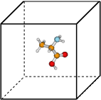
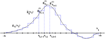
Figure 3.1: Left: Glycine amino acid in a computational box. Right: approximation of the Gaussian-type basis function by a piecewise constant function.

The molecule is embedded in a certain fixed computational box $\Omega=[-b,b]^{3}\in\mathbb{R}^{3}$, as in Fig. 3.1, left. For a given discretization parameter $n\in\mathbb{N}$, we use the equidistant $n\times n\times n$ tensor grid $\omega_{{\bf 3},n}=\{x_{\bf i}\}$, ${\bf i}\in{\cal I}:=\{1,...,n\}^{3}$, with the mesh-size $h=2b/(n+1)$. Then the Gaussian basis functions $g_{k}(x),\;x\in\mathbb{R}^{3}$, are approximated by sampling their values at the centers of discretization intervals, as in Fig. 3.1, right, using one-dimensional piecewise constant basis functions $g_{k}(x)\approx\overline{g}_{k}(x)=\prod^{3}_{\ell=1}\overline{g}_{k}^{(\ell)}(x_{\ell})$, $\ell=1,2,3$, yielding their rank-$1$ tensor representation,

$${\bf G}_{k}={\bf g}_{k}^{(1)}\otimes{\bf g}_{k}^{(2)}\otimes{\bf g}_{k}^{(3)}\in\mathbb{R}^{n\times n\times n},\quad k=1,...,N_{b}.$$ (3.1)

Let us consider the tensor calculation of the Hartree potential

$${V_{H}({x}):=\int_{\mathbb{R}^{3}}\frac{\rho({y})}{\|{x}-{y}\|}\,d{y}},$$

and the corresponding Coulomb matrix,

$$J_{km}:=\int_{\mathbb{R}^{3}}g_{k}({x})g_{m}({x})V_{H}({x})d{x},\quad k,m=1,\ldots N_{b}\quad x\in\mathbb{R}^{3},$$

where the electron density, $\rho(x)=2\sum\limits_{a=1}^{N_{orb}}(\varphi_{a})^{2}$, is represented in terms of molecular orbitals $\varphi_{a}(x)=\sum\limits_{k=1}^{N_{b}}c_{a,k}g_{k}(x)$. Given the discrete tensor representation of basis functions (3.1), the electron density is approximated using 1D Hadamard products of rank-$1$ tensors (instead of product of Gaussians),

$$\rho\approx\Theta=\sum\limits^{N_{orb}}_{a=1}\sum\limits^{N_{b}}_{k=1}\sum\limits^{N_{b}}_{m=1}c_{a,m}c_{a,k}({\bf g}_{k}^{(1)}\odot{\bf g}_{m}^{(1)})\otimes({\bf g}_{k}^{(2)}\odot{\bf g}_{m}^{(2)})\otimes({\bf g}_{k}^{(3)}\odot{\bf g}_{m}^{(3)})\in\mathbb{R}^{n\times n\times n}.$$

Further, the representation of the Newton kernel $\frac{1}{\|{x}-{y}\|}$ by a canonical rank-$R_{N}$ tensor [7] is used (see Appendix for details),

$${\bf P}_{R}=\sum\limits_{q=1}^{R_{N}}{\bf p}^{(1)}_{q}\otimes{\bf p}^{(2)}_{q}\otimes{\bf p}^{(3)}_{q}\in\mathbb{R}^{n\times n\times n}.$$ (3.2)

Since large ranks make tensor operations inefficient, the multigrid canonical-to-Tucker and Tucker-to-canonical algorithms should be applied to reduce the initial rank of $\Theta\mapsto\Theta^{\prime}$ by several orders of magnitude, from $N_{b}^{2}/2$ to $R_{\rho}\ll N_{b}^{2}/2$. Then the 3D tensor representation of the Hartree potential is calculated by using the 3D tensor product convolution, which is a sum of tensor products of 1D convolutions,

$$V_{H}\approx{\bf V}_{H}=\Theta^{\prime}\ast{\bf P}_{R}=\sum\limits_{m=1}^{R_{\rho}}\sum\limits_{q=1}^{R_{N}}c_{m}\left({\bf u}^{(1)}_{m}\ast{\bf p}^{(1)}_{q}\right)\otimes\left({\bf u}^{(2)}_{m}\ast{\bf p}^{(2)}_{q}\right)\otimes\left({\bf u}^{(3)}_{m}\ast{\bf p}^{(3)}_{q}\right).$$

The Coulomb matrix entries $J_{km}$ are obtained by 1D scalar products of ${\bf V}_{H}$ with the Galerkin basis consisting of rank-$1$ tensors,

$$J_{km}\approx\langle{\bf G}_{k}\odot{\bf G}_{m},{\bf V}_{H}\rangle,\quad k,m=1,\ldots N_{b}.$$

The cost of 3D tensor product convolution is $O(n\log n)$ instead of $O(n^{3}\log n)$ for the standard benchmark 3D convolution using the 3D FFT. Next Table shows CPU times (sec) for the Matlab computation of $V_{H}$ for H₂O molecule [38] on a SUN station using 8 Opteron Dual-Core/2600 processors (times for 3D FFT for $n\geq 1024$ are obtained by extrapolation). C2T shows the time for the canonical-to-Tucker rank reduction.

$n^{3}$	$1024^{3}$	$2048^{3}$	$4096^{3}$	$8192^{3}$	$16384^{3}$
FFT3	$\sim 6000$	–	–	–	$\sim 2$ years
$C\ast C$	$8.8$	$20.0$	$61.0$	$157.5$	$299.2$
C2T	$6.9$	$10.9$	$20.0$	$37.9$	$86.0$

Table 3.1: Times (sec) for the 3D tensor product convolution vs. 3D FFT convolution.

In a similar way, the algorithm for 3D grid-based tensor-structured calculation of 6D integrals in the exchange potential operator was introduced in [39], $K_{km}=\sum\limits^{N_{orb}}_{a=1}K_{km,a}$ with

$$K_{km,a}:=\int_{\mathbb{R}^{3}}\int_{\mathbb{R}^{3}}g_{k}(x)\frac{\varphi_{a}(x)\varphi_{a}(y)}{|x-y|}g_{m}(y)dxdy,\quad k,m=1,\ldots N_{b},$$

the contribution from the $a$-th orbital are approximated by tensor anzats,

$$K_{km,a}:=\left\langle{\bf G}_{k}\odot\left[\sum\limits_{\mu=1}^{N_{b}}c_{\mu a}{\bf G}_{\mu}\right],\left[{\bf G}_{m}\odot\sum\limits_{\nu=1}^{N_{b}}c_{\nu a}{\bf G}_{\nu}\right]\ast{\bf P}_{R}\right\rangle.$$

Here, the tensor product convolution is first calculated for each $a$th orbital, and then scalar products in canonical format yield the contributions to entries of the exchange Galerkin matrix from the $a$-th orbital.

These algorithms were employed in the first tensor-structured solver using 3D grid-based evaluation of the Coulomb and exchange matrices in 1D complexity at every step of SCF EVP iteration [40, 41]. A sequence of dyadically refined 3D Cartesian grids was used for reducing time in first iterations, with an $\varepsilon$ convergence criterion for switching to larger grids. This is a nonstandard computational scheme avoiding calculation of the two-electron integrals. The accuracy for small molecules like H₂O and CH₄ was of the order of $10^{-4}$ Hartree. Though time performance of this solver was not compatible with the standard Hartree-Fock packages it was the first proof of concept for the tensor numerical methods.

3.2 3D grid-based calculation of the two-electron integrals.

The basic tensor-structured Hartree-Fock solver employs the factorized 3D grid-based calculation of the two-electron integrals tensor, ${\bf B}=[b_{\mu\nu\kappa\lambda}]$, in the form

$$b_{\mu\nu\kappa\lambda}=\int_{\mathbb{R}^{3}}\int_{\mathbb{R}^{3}}\frac{g_{\mu}(x)g_{\nu}(x)g_{\kappa}(y)g_{\lambda}(y)}{\|x-y\|}dxdy=\left\langle{\bf G}_{\mu}\odot{\bf G}_{\nu},{\bf P}_{R}\ast\left({\bf G}_{\kappa}\odot{\bf G}_{\lambda}\right)\right\rangle_{n^{\otimes 3}},$$ (3.3)

by using univariate tensor operations. Introduce the side matrices $G^{(\ell)}$ representing on the grid the full set of canonical vectors composing the products of the Gaussian basis functions, $\{{\bf G}_{\mu}\odot{\bf G}_{\nu}\}$,

$$G^{(\ell)}=\left[{\bf g}^{(\ell)}_{\mu}\odot{\bf g}^{(\ell)}_{\nu}\right]_{1\leq\mu,\nu\leq N_{b}}\in\mathbb{R}^{n\times N_{b}^{2}}\quad\ell=1,2,3,$$

where in most of our Hartree-Fock calculations grids of size $n^{3}=32\cdot 10^{3}$ or $n^{3}=64\cdot 10^{3}$ have been used. It was found that the large matrices $G^{(\ell)}$ of size $n\times N_{b}^{2}$ (e.g. $N_{b}^{2}=40000$ for Alanine amino acid) can be approximated with high accuracy by low rank matrices with the rank parameter bounded by $R_{\ell}\leq N_{b}$ [43, 44]. The corresponding low-rank factorizations (“1D density fitting”) in the form (for $\ell=1,2,3$)

$$G^{(\ell)}\cong U^{(\ell)}{V^{(\ell)}}^{T},\quad U^{(\ell)}\in\mathbb{R}^{n\times R_{\ell}},\quad V^{(\ell)}\in\mathbb{R}^{N^{2}_{b}\times R_{\ell}},$$ (3.4)

is computed by the truncated Cholesky decomposition of the symmetric, positive definite $G^{(\ell)}{G^{(\ell)}}^{T}$ (see [43, 44] for more details).

Based on factorization (3.4), the number of convolutions in (3.3) is reduced dramatically from $N_{b}^{2}$ to $N_{b}$ at most (say from $40000$ to $200$). In fact, using canonical factors from the rank-$R$ canonical tensor ${\bf P}_{R}$ representing the Newton kernel (3.2) (see (7.8) in Appendix) we, first, precompute the set of “convolution“ matrices for every space variable $\ell,\;\ell=1,2,3$,

$$M_{k}^{(\ell)}={U^{(\ell)}}^{T}({\bf p}_{k}^{(\ell)}\ast_{n}U^{(\ell)})\in\mathbb{R}^{R_{\ell}\times R_{\ell}},\quad k=1,...,R,$$ (3.5)

which includes the convolution products with $R_{\ell}\leq N_{b}$ column vectors of the matrix $U^{(\ell)}\in\mathbb{R}^{n\times R_{\ell}}$ instead of $N_{b}^{2}/2$ convolutions in the initial formulation.

Given matrices $M_{k}^{(\ell)}$, then the resulting $4$-th order TEI tensor is represented in a matrix form

$$B=mat({\bf{B}})\cong B_{\varepsilon}:=\sum\limits^{R}_{k=1}\odot^{3}_{\ell=1}V^{(\ell)}M_{k}^{(\ell)}{V^{(\ell)}}^{T}\in\mathbb{R}^{N_{b}^{2}\times N_{b}^{2}}.$$

The above nonstandard factorization of the TEI matrix $B$ allows to reduce dramatically the computational cost of the standard Cholesky factorization schemes [29, 5] applied to the reduced-rank symmetric positive definite matrix $B$. In fact, the low-rank Cholesky decomposition of $B$ is calculated in the following sequence. First, the diagonal elements of $B$ are calculated as

$$B(i,i)=\sum\limits^{R}_{k=1}\odot^{3}_{\ell=1}V^{(\ell)}(i,:)M_{k}^{(\ell)}{V^{(\ell)}(:,i)}^{T}.$$

Then the selected columns of the matrix $B$, required for the rank-truncated Cholesky factorization scheme, are computed by the following fast tensor operations

$$B(:,j^{\ast})=\sum\limits^{R}_{k=1}\odot^{3}_{\ell=1}V^{(\ell)}M_{k}^{(\ell)}{V^{(\ell)}(:,j^{\ast})}^{T},$$

leading to representation of the matrix $B$ in the form of rank-$R_{B}$ approximate decomposition [43, 44]

$$B:=[b_{\mu\nu,\kappa\lambda}]\approx LL^{T},\quad\mbox{ with }\quad L\in\mathbb{R}^{N_{b}^{2}\times R_{B}},\;R_{B}\sim N_{b}.$$

This algorithm is much faster than the direct Cholesky decomposition of the matrix $B$ with on-the-fly computation of the required column vectors.

$n^{3}$	$16384^{3}$	$32768^{3}$	$65536^{3}$	$131072^{3}$
mesh (bohr)	$0.0024$	$0.0012$	$6\cdot 10^{-4}$	$3\cdot 10^{-4}$
Had. prod.	$1.6$	$3.4$	$12$	$19$
Density fit.	$0.5$	$1.0$	$2.0$	$4.0$
3D Conv. time	$69$	$151$	$698$	$496$
Chol. time	$2.2$	$2.2$	$2.2$	$2.2$

Table 3.2: Times (sec) for 3D grid-based calculation of the directional density fitting and the TEI for H₂O molecule.

Table 3.2 represents times (sec) for 3D grid-based calculation of the directional density fitting and the TEI tensor (electron repulsion integrals) for H₂O molecule in a box $[-20,20]^{3}$ bohr³, performed in Matlab on a 2-Intel Xeon Hexa-Core/2677. Time for convolution integrals in (3.5) scales almost linearly in the $1D$ grid-size $n$ as expected by theory.

3.3 Core Hamiltonian.

The Galerkin representation of the 3D Laplace operator in the nonlocal Gaussian basis $\{g_{k}(x)\}_{1\leq k\leq N_{b}}$, $x\in\mathbb{R}^{3}$, leads to the fully populated matrix $A_{g}=[a_{km}]\in\mathbb{R}^{N_{b}\times N_{b}}$. Tensor calculation of the matrix entries $a_{km}$ for the discrete Laplacian $A_{g}$ in the separable Gaussian basis is reduced to 1D matrix operations [45] involving the FEM Laplacian $\Delta_{3}$, defined on $n\times n\times n$ grid,

$$\Delta_{3}=\Delta_{1}^{(1)}\otimes I^{(2)}\otimes I^{(3)}+I^{(1)}\otimes\Delta_{1}^{(2)}\otimes I^{(3)}+I^{(1)}\otimes I^{(2)}\otimes\Delta_{1}^{(3)},$$

where $\Delta_{1}=\frac{1}{h}tridiag\{-1,2,-1\}$. Specifically, we have

$${a}_{km}=\langle\Delta_{3}{\bf G}_{k},{\bf G}_{m}\rangle,$$

where ${\bf G}_{k}$ is the tensor representation of Gaussian basis functions using the piecewise linear finite elements. In the case of large $n\times n\times n$ grids, this calculation can be implemented with logarithmic cost in $n$ by using the low-rank QTT representation of the large matrix $\Delta_{3}$, see [32].

For tensor calculation of the nuclear potential operator

$$V_{c}(x)=-\sum_{\alpha=1}^{M}\frac{Z_{\alpha}}{\|{x}-a_{\alpha}\|},\quad Z_{\alpha}>0,\;\;x,a_{\alpha}\in\mathbb{R}^{3},$$

we apply the rank-$1$ windowing operator, ${\cal W}_{\alpha}={\cal W}_{\alpha}^{(1)}\otimes{\cal W}_{\alpha}^{(2)}\otimes{\cal W}_{\alpha}^{(3)}$, for shifting the reference Newton kernel $\widetilde{\bf P}_{R}\in\mathbb{R}^{2n\times 2n\times 2n}$ according to the coordinates of nuclei in a molecule (see Section 5 and Appendix). Then the resulting nuclear potential, ${\bf P}_{c}\in\mathbb{R}^{n\times n\times n}$, is obtained as a direct tensor sum of shifted potentials [45],

$${\bf P}_{c}=\sum_{\alpha=1}^{M}Z_{\alpha}{\cal W}_{\alpha}\widetilde{\bf P}_{R}$$

$$=\sum_{\alpha=1}^{M}Z_{\alpha}\sum\limits_{q=1}^{R}{\cal W}_{\alpha}^{(1)}\widetilde{\bf p}^{(1)}_{q}\otimes{\cal W}_{\alpha}^{(2)}\widetilde{\bf p}^{(2)}_{q}\otimes{\cal W}_{\alpha}^{(3)}\widetilde{\bf p}^{(3)}_{q}.$$

This leads to the following representation of the Galerkin matrix, $V_{c}=[\overline{v}_{km}]$, by tensor operations

$$\overline{v}_{km}=\int_{\mathbb{R}^{3}}V_{c}(x)\overline{g}_{k}(x)\overline{g}_{m}(x)dx\approx\langle{\bf G}_{k}\odot{\bf G}_{m},{\bf P}_{c}\rangle,\quad 1\leq k,m\leq N_{b}.$$

Figure 3.2, left, shows several vectors of the canonical representation of the Coulomb kernel along one of variables. Figure 3.2, right, represents the cross-section of the resulting nuclear potential ${\bf P}_{c}$ for C₂H₅OH molecule.

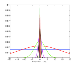
Figure 3.2: Left: Several vectors of the canonical representation of the Newton kernel along one of variables. Right: calculated sum of the nuclear potentials for ethanol molecule.

3.4 Black-box tensor solver.

The tensor-structured Hartree-Fock solver [45] based on factorized calculation of the two-electron integrals [43] includes efficient tensor implementation of the MP2 energy correction [44] scheme. Though it is yet implemented in Matlab, its performance in time and accuracy is compatible with the standard packages based on analytical evaluation of the two-electron integrals. Due to 1D complexity of all calculations, it enables 3D grids of the size $10^{15}$, yielding mesh size of the order of atomic radii, $10^{-4}$ Å. That ensures high accuracy of calculations, which is controlled by the $\varepsilon$-ranks of tensor truncation.

The solver works in a black-box way: input the grid-based basis-functions and coordinates of nuclei in a molecule and start the program. Calculation of TEI for H₂O on grids $32768^{3}$ takes two minutes on a laptop. The time for TEI with $n^{3}=131072^{3}$ for Alanine amino acid takes approximately one hour in Matlab, including incorporated density fitting.

Next examples compare the results from benchmark Molpro program with calculations by the tensor-based solver by using the same Gaussian basis, but now discretized on 3D Cartesian grid. For all molecules we use the ”cc-pVDZ“ Gaussian basis set. The core Hamiltonian part in these calculations is taken from Molpro. Note that since in the tensor solver the density fitting is included in ”blind“ calculation of TEI, it is not easy to compare the CPU times of our calculations with those in ”ab-initio“ procedure in the standard programs, because the density fitting step there is usually considered as off-line pre-computing.

Figure 3.3 shows convergence history of ab initio iterations for H₂O molecule (cc-pVDZ-41), where TEI is computed on the 3D grid of size $131072^{3}$, while Figure 3.3 (right) presents the zoom of the left graphic at the last 20 iterations. The ground state energy from Molpro is shown by the black dashed line.

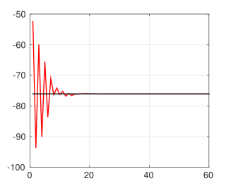
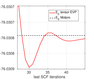
Figure 3.3: Left: SCF EVP iteration for H₂O; Right: convergence of the ground state energy vs. final $20$ iterations for H₂O.

Figure 3.4 (left) shows the SCF EVP iteration for Glycine amino acid (cc-pVDZ-170), where dashed line indicates convergence of the residual and the red solid line shows convergence of the error to ground state energy from MOLPRO package with the same basis set. Figure 3.4 (right) illustrates the convergence of the ground state energy at final $20$ iterations for Glycine, dashed line is the energy from Molpro.

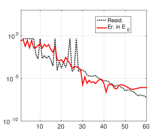
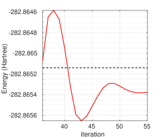
Figure 3.4: Left: SCF EVP iteration for Glycine (C₂H₅NO₂) molecule. Right: convergence of the ground state energy at final $20$ iterations for Glycine molecule.

The second row in Table 3.3 represents times (sec) for one step of SCF iteration in ab-initio solution of the Hartree Fock EVP for H₂O (cc-pVDZ-41), H₂O₂ (cc-pVDZ-68), and C₂H₅NO₂ (cc-pVDZ-170) molecules while the first row shows the molecular parameters, number of orbitals and basis functions. Next two rows show the relative difference $\Delta E_{0,g}={|E_{0,g}-E_{0}|}/{|E_{0}|}$, between the grid-based ground state energy, $E_{0,g}$ and $E_{0}$ from Molpro with the same basis sets. This numerics demonstrates that in the case of fine enough spacial $n\times n\times n$-grids the accuracy in 7 - 8 digits (i.e. relative accuracy about $10^{-7}-10^{-8}$) can be achieved for moderate size molecules up to small amino acids.

	H2O	H2O2	C2H5NO2
$N_{orb}$, $N_{b}$	$5$; $41$	$9$; $68$	$20$; $170$
Time	$0.35$	$0.55$	$6.0$
$\Delta E_{0,g},(65536^{3})$	$3.0\cdot 10^{-7}$	$8.0\cdot 10^{-8}$	$9.1\cdot 10^{-7}$
$\Delta E_{0,g},(131072^{3})$	$1.4\cdot 10^{-7}$	$3.9\cdot 10^{-8}$	$8.0\cdot 10^{-7}$

Table 3.3: Time (sec) for one ab-initio SCF EVP iteration and accuracy of ab-initio solution with respect to grid-size in TEI calculations. Matlab on an Intel Xeon X5650.

All calculations are performed in the computational box of size $[-20,20]^{3}$ bohr³. This tensor-based solver can be considered as the computational tool for trying the alternatives to Gaussian-type basis sets.

4 From MP2 energy correction to excited states

4.1 MP2 correction scheme by using tensor formats

Given the set of Hartree-Fock molecular orbitals $\{C_{p}\}$ and the corresponding energies $\{\varepsilon_{p}\}$, $p=1,2,...,N_{b}$, where $\{C_{i}\}$ and $\{C_{a}\}$ denote the occupied and virtual orbitals, respectively. First, one has to transform the TEI matrix ${B}=[b_{\mu\nu,\lambda\sigma}]$, corresponding to the initial AO basis set, to those represented in the molecular orbital (MO) basis,

$${V}=[v_{ia,jb}]:\quad v_{iajb}=\sum\limits_{\mu,\nu,\lambda,\sigma=1}^{N_{b}}C_{\mu i}C_{\nu a}C_{\lambda j}C_{\sigma b}b_{\mu\nu,\lambda\sigma},$$ (4.1)

where $a,b\in{\cal I}_{v}$, $i,j\in{\cal I}_{o}$, and ${\cal I}_{o}:=\{1,...,N_{orb}\}$, ${\cal I}_{v}:=\{N_{orb}+1,...,N_{b}\}$, with $N_{orb}$ denoting the number of occupied orbitals. In the following, we shall use the notation

$$N_{v}=N_{b}-N_{orb},\quad\quad N_{ov}=N_{orb}N_{v}.$$

The straightforward computation of the matrix $V$ by above representation makes the dominating impact to the overall numerical cost of order $O(N_{b}^{5})$. The method of complexity $O(N_{b}^{4})$ based on the low-rank tensor decomposition of the matrix $V$ was introduced in [44]. Indeed, it can be shown that the rank $R_{B}=O(N_{b})$ approximation to the TEI matrix $B\approx LL^{T},$ with the $N\times R_{B}$ Cholesky factor $L$, allows to introduce the low-rank representation of the matrix ${V}$, (see [44] and [6])

$$V=L_{V}L_{V}^{T},\quad L_{V}\in\mathbb{R}^{N_{ov}\times R_{B}},$$

and then reduce the asymptotic complexity of calculations to $O(N_{b}^{4})$.

Given the tensor ${\bf V}=[v_{iajb}]$, the second order MP2 perturbation to the HF energy is calculated by

$$E_{MP2}=-\sum\limits_{a,b\in I_{vir}}\sum\limits_{i,j\in I_{occ}}\frac{v_{iajb}(2v_{iajb}-v_{ibja})}{\varepsilon_{a}+\varepsilon_{b}-\varepsilon_{i}-\varepsilon_{j}},$$ (4.2)

where the real numbers $\varepsilon_{k}$, $k=1,...,N_{b}$, represent the HF eigenvalues.

Introducing the so-called doubles amplitude tensor ${\bf T}$,

$${\bf T}=[t_{iajb}]:\;t_{iajb}=\frac{(2v_{iajb}-v_{ibja})}{\varepsilon_{a}+\varepsilon_{b}-\varepsilon_{i}-\varepsilon_{j}},\quad a,b\in I_{vir};\;i,j\in I_{occ},$$

the MP2 perturbation takes the form of a simple scalar product of tensors,

$$E_{MP2}=-\langle{\bf V},{\bf T}\rangle=-\langle{\bf V}\odot{\bf T},{\bf 1}\rangle,$$

where ${\bf 1}$ denotes the rank-$1$ all-ones tensor. Introducing the low $\varepsilon$-rank reciprocal “energy“ tensor

$${\bf E}=[e_{abij}]:=\left[\frac{1}{\varepsilon_{a}+\varepsilon_{b}-\varepsilon_{i}-\varepsilon_{j}}\right],\quad a,b\in I_{vir};\;i,j\in I_{occ},$$ (4.3)

and the partly transposed tensor (transposition in indices $a$ and $b$)

$${\bf V}^{\prime}=[v^{\prime}_{iajb}]:=[v_{ibja}],$$

allows to decompose the doubles amplitude tensor ${\bf T}$ as follows

$${\bf T}={\bf T}^{(1)}+{\bf T}^{(2)}=2{\bf V}\odot{\bf E}-{\bf V}^{\prime}\odot{\bf E}.$$ (4.4)

Notice that the denominator in (4.2) remains strongly positive if $\varepsilon_{a}>0$ for $a\in I_{vir}$ and $\varepsilon_{i}<0$ for $i\in I_{occ}$. The latter condition (nonzero homo lumo gap) allows to prove the low $\varepsilon$-rank decomposition of the tensor ${\bf E}$ [43, 44].

Each term in the right-hand side in (4.4) can be treated separately by using ranks-structured tensor decompositions of ${\bf V}$ and ${\bf E}$, possibly combined with various symmetries and data sparsity. Numerical tests illustrating the tensor approach to the MP2 energy correction are presented in [44].

4.2 Toward low-rank approximation of the Bethe-Salpeter equation for calculation of excited states

One of the commonly used approaches for calculation of the excited states in molecules and solids, along with the time-dependent DFT, is based on the solution of the Bethe-Salpeter equation (BSE), see for example [11, 60]. The BSE approach leads to the challenging computational task on the solution of the eigenvalue problem for determining the excitation energies $\omega_{n}$, governed by a large fully populated matrix of size $O(N^{2}_{ov})\approx O(N^{2}_{b})$,

$$\begin{pmatrix}{A}&{B}\\ {B}^{\ast}&{A}^{\ast}\\ \end{pmatrix}\begin{pmatrix}{\bf x}_{n}\\ {\bf y}_{n}\\ \end{pmatrix}=\omega_{n}\begin{pmatrix}{I}&{0}\\ {0}&{-I}\\ \end{pmatrix}\begin{pmatrix}{\bf x}_{n}\\ {\bf y}_{n}\\ \end{pmatrix},$$ (4.5)

so that the computation of the entire spectrum is prohibitively expensive. Here the large matrix blocks of size $N_{ov}\times N_{ov}$ take a form

$$A=\boldsymbol{\Delta\varepsilon}+V-\overline{W},\quad B={V}-\widetilde{W},$$

where the diagonal ”energy” matrix is defined by

$$\boldsymbol{\Delta\varepsilon}=[\Delta\varepsilon_{ia,jb}]\in\mathbb{R}^{N_{ov}\times N_{ov}}:\quad\Delta\varepsilon_{ia,jb}=(\varepsilon_{a}-\varepsilon_{i})\delta_{ij}\delta_{ab},$$

while the matrices $\overline{W}=[\overline{w}_{ia,jb}]$ and $\widetilde{W}=[\widetilde{w}_{ia,jb}]$ are determined by permutation of the so-called static screened interaction matrix ${W}=[{w}_{ia,jb}]$, via $\overline{w}_{ia,jb}={w}_{ij,ab}$, and $[\widetilde{w}_{ia,jb}]=[{w}_{ib,aj}]$, respectively. In turn, the forth order tensor ${\bf W}=[{w}_{iajb}]$ is constructed by certain linear transformations of the tensor ${\bf V}=[v_{iajb}]$, see [11, 60].

A number of numerical methods for structured eigenvalue problems have been discussed in the literature [50, 4, 14, 54].

The tensor approach to the solution of the partial BSE eigenvalue problem for equation (4.5) proposed in [6] suggests to compute the reduced basis set by solving the simplified eigenvalue problem via the low-rank plus diagonal approximation to the matrix blocks $A$ and $B$, and then solve spectral problem for the subsequent Galerkin projection of the initial system (4.5) to this reduced basis. This procedure relies entirely on multiplication of the simplified BSE matrix with vectors.

It was demonstrated on the examples of moderate size molecules[6] that a small reduced basis set, obtained by separable approximation with the rank parameters of about several tens, allows to reveal several lowest excitation energies and respective excited states with the accuracy about $0.1$eV - $0.02$eV.

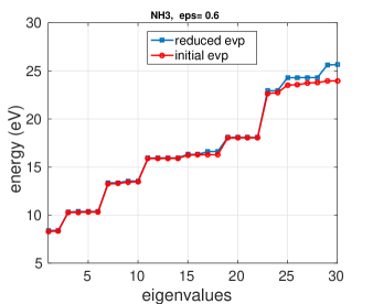
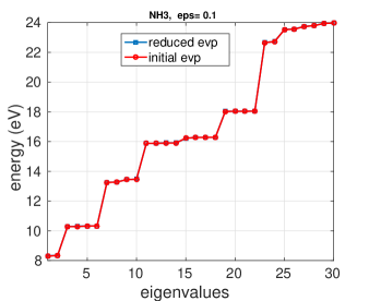
Figure 4.1: Comparison of $m_{0}=30$ lower eigenvalues for the reduced and exact BSE systems for NH₃ molecule: $\varepsilon=0.6$, left; $\varepsilon=0.1$, right.

Figure 4.1 illustrates the BSE energy spectrum of the NH₃ molecule (based on HF calculations with cc-pDVZ-48 GTO basis) for the lowest $N_{red}=30$ eigenvalues vs. the rank truncation parameter $\varepsilon=0.6$ and $0.1$, where the ranks of $V$ and the BSE matrix block $W$ are $4$, $5$ and $28$, $30$, respectively. For the choice $\varepsilon=0.6$ and $\varepsilon=0.1$, the error in the 1st (lowest) eigenvalue for the solution of the problem in reduced basis is about $0.11$eV and $0.025$eV, correspondingly. The CPU time in the laptop Matlab implementation of each example is about $5$sec.

5 Tensor approach to simulation of large crystalline clusters

In this section, we briefly discuss the generalization of the tensor-based Hartree-Fock solver to the case of large lattice structured and periodic systems [46, 47] arising in the numerical modeling of crystalline, metallic and polymer type compounds.

5.1 Fast tensor calculation of a lattice sum of interaction potentials

One of the challenges in the numerical treatment of large molecular systems is the summation of long-range potentials allocated on large 3D lattices. The conventional Ewald summation techniques based on a separate evaluation of contributions from the short- and long-range parts of the interaction potential exhibit $O(L^{3}\log L)$ complexity scaling for a cubic $L\times L\times L$ 3D lattice.

In the contrary, the main idea of the novel tensor summation method introduced in [46, 48] suggests to benefit from the low-rank tensor decomposition of the generating kernel approximated on the fine $n\times n\times n$ representation grid in the 3D computational box $\Omega_{L}$. This allows to completely decouple the 3D sum into the three independent $1$D summations, thus reducing drastically the numerical expenses. The resultant potential sum, which now requires only $O(n)$ storage and $O(nL)$ computational demands, is represented by a few assembled canonical/Tucker $n$-vectors of complicated shape (see Figure 5.1), where $n$ is the univariate grid size for a cubic 3D lattice.

For ease of exposition, we consider the electrostatic potential the nuclear potential of a single hydrogen atom, $V_{c}(x)=\frac{Z}{\|x\|}$. Define the scaled unit cell, $\Omega_{0}=[0,b]^{3}$, of size $b\times b\times b$ and consider a sum of interaction potentials in a symmetric computational box

$$\Omega_{L}=B\times B\times B,\quad\mbox{with}\quad B={b}[-\frac{L}{2},\frac{L}{2}],\quad L=2L_{0}\in\mathbb{N},$$

consisting of a union of $L\times L\times L$ unit cells $\Omega_{\bf k}$, obtained from $\Omega_{0}$ by a shift along the lattice vector $b{\bf k}$, where ${\bf k}=(k_{1},k_{2},k_{3})\in\mathbb{Z}^{3}$, such that $k_{\ell}\in{\cal K}:={\cal K}_{-}\cup{\cal K}_{+}$ for $\ell=1,2,3$ with ${\cal K}_{-}:=\{-1,...,-\frac{L}{2}\}$ and ${\cal K}_{+}:=\{0,1,...,\frac{L}{2}-1\}$. Hence, we have $\Omega_{L}=\bigcup_{k_{1},k_{2},k_{3}\in{\cal K}}\Omega_{\bf k}\in\mathbb{R}^{3}$.

Recall that $b=nh$, where $h>0$ is the fine mesh size that is the same for all spatial variables, and $n$ is the number of grid points for each variable. We also define the accompanying domain $\widetilde{\Omega}_{L}$ obtained by scaling of ${\Omega}_{L}$ with the factor of $2$, $\widetilde{\Omega}_{L}=2{\Omega}_{L}$, and, similar to (7.8), introduce the respective rank-$R$ reference (master) tensor

$$\widetilde{\bf P}=\sum\limits_{q=1}^{R}\widetilde{\bf p}^{(1)}_{q}\otimes\widetilde{\bf p}^{(2)}_{q}\otimes\widetilde{\bf p}^{(3)}_{q}\in\mathbb{R}^{2n\times 2n\times 2n},$$ (5.1)

approximating $\frac{1}{\|{x}\|}$ in $\widetilde{\Omega}_{L}$ on a $2n\times 2n\times 2n$ representation grid with mesh size $h$.

Let us consider a sum of single Coulomb potentials on a $L\times L\times L$ lattice,

$$V_{c_{L}}(x)=\sum\limits_{k_{1},k_{2},k_{3}\in{\cal K}}\frac{Z_{1}}{\|{x}-a_{1}(k_{1},k_{2},k_{3})\|},\quad x\in\Omega_{L}\in\mathbb{R}^{3}.$$ (5.2)

The assembled tensor approach applies to the potentials defined on $n\times n\times n$ 3D Cartesian grid. It reduces the sum over a rectangular 3D lattice, ${\bf P}_{c_{L}}\in\mathbb{R}^{n\times n\times n}$,

$${\bf P}_{c_{L}}=\sum\limits_{{\bf k}\in{\cal K}^{3}}{\cal W}_{\nu({\bf k})}\widetilde{\bf P}=\sum\limits_{k_{1},k_{2},k_{3}\in{\cal K}}\sum\limits_{q=1}^{R}{\cal W}_{({\bf k})}(\widetilde{\bf p}^{(1)}_{q}\otimes\widetilde{\bf p}^{(2)}_{q}\otimes\widetilde{\bf p}^{(3)}_{q}),$$

to the summation of directional vectors for the canonical decomposition of shifted single Newton kernels [46],

$${\bf P}_{c_{L}}=\sum\limits_{q=1}^{R}(\sum\limits_{k_{1}\in{\cal K}}{\cal W}_{({k_{1}})}\widetilde{\bf p}^{(1)}_{q})\otimes(\sum\limits_{k_{2}\in{\cal K}}{\cal W}_{({k_{2}})}\widetilde{\bf p}^{(2)}_{q})\otimes(\sum\limits_{k_{3}\in{\cal K}}{\cal W}_{({k_{3}})}\widetilde{\bf p}^{(3)}_{q}),$$ (5.3)

where ${\cal W}_{\nu({\bf k})}={\cal W}_{{k_{1}}}\otimes{\cal W}_{{k_{2}}}\otimes{\cal W}_{{k_{3}}}$ is the shift-and-windowing (onto $\Omega_{L}$) separable transform along the ${\bf k}$-grid. Remarkably that the rank of the resulting sum is the same as for the $R$-term canonical reference tensor (5.1) representing the single Newton kernel.

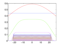
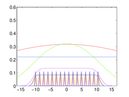
Figure 5.1: Assembled $x$- and $y$-axis canonical vectors for a cluster of $32\times 16\times 8$ Hydrogen nuclei.

The numerical cost and storage size are bounded by $O(RLn)$ and $O(Rn)$, respectively, where $n=n_{0}L$, and $n_{0}$ is the grid size in the unit cell.

Figures 5.1 and 5.2 represent the shape of assembled canonical vectors for the cluster of $32\times 16\times 8$ Hydrogen nuclei. Size of the computational box is $62\times 32\times 22$ bohr³. Here the empty interval between the lattice and the boundary of the computational box equals to $6$ bohr.

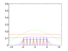
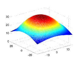
Figure 5.2: Assembled $z$-axis canonical vectors for a cluster of $32\times 16\times 8$ Hydrogen nuclei. Assembled canonical sum of the Newton potentials for this cluster.

The next table represents CPU times for the lattice summation of the Newton kernels over $L\times L\times L$ cubic box, with very fine $n\times n\times n$ representation grid.

$L^{3}$	$4096$	$32768$	$262144$	$2097152$
Time (sec.)	$1.8$	$0.8$	$3.1$	$15.8$
3D grid size, $n^{3}$	$5632^{3}$	$9728^{3}$	$17920^{3}$	$34304^{3}$

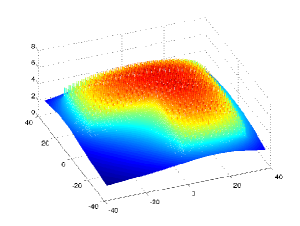
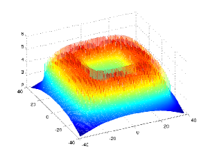
Figure 5.3: Assembled canonical sum of the Coulomb potentials on the $L$-shaped (left) and $O$-shaped (right) sub-lattices of a $32\times 32\times 1$ lattice.

The summation method in the canonical format was extended to the Tucker tensors which allows the principal generalization of this techniques to the case of rather complicated lattices with defects (Theorem 3.2, [48]), so that the resulting sum takes a form

$${\bf T}_{c_{L}}=\sum\limits_{m_{1}=1}^{r_{1}}\sum\limits_{m_{2}=1}^{r_{2}}\sum\limits_{m_{3}=1}^{r_{3}}b_{m_{1},m_{2},m_{3}}(\sum\limits_{k_{1}\in{\cal K}}{\cal W}_{({k_{1}})}\widetilde{\bf t}^{(1)}_{m_{1}})\otimes(\sum\limits_{k_{2}\in{\cal K}}{\cal W}_{({k_{2}})}\widetilde{\bf t}^{(2)}_{m_{2}})\otimes(\sum\limits_{k_{3}\in{\cal K}}{\cal W}_{({k_{3}})}\widetilde{\bf t}^{(3)}_{m_{3}}),$$

where $\widetilde{\bf t}^{(\ell)}_{m_{\ell}}$, $\ell=1,2,3$, represents the Tucker vectors of the rank-${\bf r}$ master tensor approximating the Newton kernel $\frac{1}{\|{x}\|}$ in $\widetilde{\Omega}_{L}$ on a $2n\times 2n\times 2n$ representation grid.

In the case of defected lattices the increasing rank of the final sum of Tucker tensors can be reduced by the stable ALS based algorithms applicable to the Tucker tensors (see [47]). The particular examples of the lattice geometries suitable for our approach are presented in Figure 5.3, see [47] for more detailed discussion.

For the reduced Hartree-Fock equation, where the Fock operator is confined to the core Hamiltonian, the tensor-structured block-circulant representation of the Fock matrix was introduced[47] that allows the special low-rank approximation of the matrix blocks. This opens the way for the numerical treatment of large eigenvalue problems with structured matrices arising in the solution of the Hartree-Fock equation for large crystalline systems with defects.

5.2 Interaction energy of long-range potentials on finite lattices

Given the nuclear charges $\{{Z_{\bf k}}\}$, centered at points ${x}_{\bf k}$, ${\bf k}\in{\cal K}^{3}$, located on a $L\times L\times L$ lattice ${\cal L}_{L}=\{{x}_{\bf k}\}$ with the step-size $b$, the interaction energy of the total electrostatic potential of these charges is defined by the lattice sum

$$E_{L}=\frac{1}{2}\sum\limits_{{\bf k},{\bf j}\in{\cal K},{\bf k}\neq{\bf j}}\frac{Z_{\bf k}Z_{\bf j}}{\|{x}_{\bf j}-{x}_{\bf k}\|},\quad\mbox{i.e. for}\quad\|{x}_{\bf j}-{x}_{\bf k}\|\geq b.$$ (5.4)

The fast and accurate computation of electrostatic interaction energy (as well as the related forces and stresses) is one of the difficult tasks in computer modeling of macromolecular structures like finite crystal, and biological systems.

The tensor summation scheme (5.3) can be directly applied to this computational problem. In what follows we show that (5.4) can be treated as a particular case of the previous scheme served for calculation of (5.2) on a fine spacial grid. For this discussion, we assume that all charges are equal, ${Z_{\bf k}}=Z$.

First, notice that the rank-$R$ reference tensor $h^{-3}\widetilde{\bf P}$ defined in (5.1) approximates with high accuracy $O(h^{2})$ the (and its shifted version) Coulomb potential $\frac{1}{\|{x}\|}$ in $\widetilde{\Omega}_{L}$ (for $\|{x}\|\geq b$ that is required for the energy expression) on the fine $2n\times 2n\times 2n$ representation grid with mesh size $h$. Likewise, the tensor $h^{-3}{\bf P}_{c_{L}}$ approximates the potential sum $V_{c_{L}}(x)$ on the same fine representation grid including the lattice points ${x}_{\bf k}$.

We propose to evaluate the energy expression (5.4) by using tensor sums as in (5.3), but now applied to a small sub-tensor of the rank-$R$ canonical reference tensor $\widetilde{\bf P}$, that is $\widetilde{\bf P}_{L}:=[\widetilde{\bf P}_{|x_{\bf k}}]\in\mathbb{R}^{2L\times 2L\times 2L}$, obtained by tracing of $\widetilde{\bf P}$ at the accompanying lattice of the double size $2L\times 2L\times 2L$, i.e. ${\cal\widetilde{L}}_{L}=\{x_{\bf k}\}\cup\{x_{{\bf k}^{\prime}}\}\in\widetilde{\Omega}_{L}$. Here $\widetilde{\bf P}_{|x_{\bf k}}$ denotes the tensor entry corresponding to the ${\bf k}$-th lattice point designating the atomic center $x_{\bf k}$. We are interested in the computation of the rank-$R$ tensor $\widehat{\bf P}_{c_{L}}=[{{\bf P}_{c_{L}}}_{|x_{\bf k}}]_{{\bf k}\in{\cal K}}\in\mathbb{R}^{L\times L\times L}$, where ${{\bf P}_{c_{L}}}_{|x_{\bf k}}$ denotes the tensor entry corresponding to the ${\bf k}$-th lattice point on ${\cal L}_{L}$. The tensor $\widehat{\bf P}_{c_{L}}$ can be computed at the expense $O(L^{2})$ by

$$\widehat{\bf P}_{c_{L}}=\sum\limits_{q=1}^{R}(\sum\limits_{k_{1}\in{\cal K}}{\cal W}_{({k_{1}})}\widetilde{\bf p}^{(1)}_{L,q}\otimes\sum\limits_{k_{2}\in{\cal K}}{\cal W}_{({k_{2}})}\widetilde{\bf p}^{(2)}_{L,q}\otimes\sum\limits_{k_{3}\in{\cal K}}{\cal W}_{({k_{3}})}\widetilde{\bf p}^{(3)}_{L,q}).$$

This leads to the representation of the energy sum (5.4) with accuracy $O(h^{2})$ in a form

$$E_{L}=\frac{Z^{2}h^{-3}}{2}(\langle\widehat{\bf P}_{c_{L}},{\bf 1}\rangle-\sum\limits_{{\bf k}\in{\cal K}}{\bf P}_{|x_{\bf k}=0}),$$

where the first term in brackets represents the full canonical tensor lattice sum restricted to the ${\bf k}$-grid composing the lattice ${\cal L}_{L}$, while the second term introduces the correction at singular points ${x}_{\bf j}-{x}_{\bf k}=0$. Here ${\bf 1}\in\mathbb{R}^{L\times L\times L}$ is the all-ones tensor. By using the rank-$1$ tensor ${\bf P}_{0L}={\bf P}_{|x_{\bf k}=0}{\bf 1}$, the correction term can be represented by a simple tensor operation

$$\sum\limits_{{\bf k}\in{\cal K}}{\bf P}_{|x_{\bf k}=0}=\langle{\bf P}_{0L},{\bf 1}\rangle.$$

Finally, the interaction energy $E_{L}$ allows the representation

$$E_{L}=\frac{Z^{2}h^{-3}}{2}(\langle\widehat{\bf P}_{c_{L}},{\bf 1}\rangle-\langle{\bf P}_{0L},{\bf 1}\rangle),$$ (5.5)

that can be implemented in $O(L^{2})\ll L^{3}\log L$ complexity by tensor operations with the rank-$R$ canonical tensors in $\mathbb{R}^{L\times L\times L}$.

Table 5.1 illustrates the performance of the algorithm described above. We compare the exact value computed by (5.4) with the approximate tensor representation in (5.5) computed on the fine representation grid with $n=n_{0}L$, $n_{0}=128$. We consider the lattices consisting of Hydrogen atoms with interatomic distance $2$ bohr. The size of the largest 3D lattice with $256^{3}$ potentials is of the size $256\cdot 2+6$ bohr, which is more than $20$ nanometers.

$L^{3}$	Total	Ts	Ttens.	$E_{L}$	err.
$24^{3}$	$13824$	$37$	$1.2$	$3.7\cdot 10^{6}$	$2\cdot 10^{-8}$
$32^{3}$	$32768$	$250$	$1.5$	$1.5\cdot 10^{7}$	$1.5\cdot 10^{-9}$
$48^{3}$	$110592$	$3374$	$2.8$	$1.12\cdot 10^{8}$	0
$64^{3}$	$262144$	-	$5.7$	$5.0\cdot 10^{8}$	-
$128^{3}$	$2097152$	-	$13.5$	$1.6\cdot 10^{10}$	-
$256^{3}$	$16777216$	-	$68.2$	$5.2\cdot 10^{11}$	-

Table 5.1: Comparison of times for the standard (T_s) and tensor-based (T_tens.) calculation of the interaction energy for the lattice electrostatic potentials. Matlab on an Intel Xeon X5650.

The presented approach for fast calculation of the interaction energy can extended to the case of non-uniform rectangular lattices and, under certain assumptions, to the case of non-equal nuclear charges $Z_{\bf k}$. Moreover, it applies to many other types of spherically symmetric interaction potentials, for example, to shielded Coulomb interaction or van der Waals attraction sums corresponding to the distance function $\|x\|^{-2}$ and $\|x\|^{-6}$, respectively.

6 Conclusions

The goal of this paper is to attract interest of the specialists in computational quantum chemistry to recent results and open questions of the grid-based tensor approach in electronic structure calculations. Here we focus mostly on the description of main mathematical and algorithmic aspects of the tensor decomposition schemes and demonstrate their benefits in some applications.

The scope of applications which can be regarded as consistent, ranges from the Hartree-Fock energy for moderate size molecules, including “blind” calculation of TEI tensor with incorporated algebraic density fitting, to calculation of the excited states for molecules, and up to a unique superfast method for calculating the lattice potential sums and the interaction energy of long range potentials on a lattice in a finite volume. Tensor approach allows to treat above problems using moderate computational facilities. All numerics given in the paper presents implementations in Matlab.

The described numerical tools are not restricted to the applications presented here, but can be applied to various hard computational problems in (post) Hartree-Fock calculations related to accurate evaluation of multidimensional integrals, and efficient storage and manipulations with large multivariate data arrays.

The presented method for summation of long-range potentials with sub-linear computational cost does not have analogues in what is used so far in computational quantum chemistry and can have a good future. For example, it can be useful in modeling of large finite molecular structures like nanostructures or quantum dots, where the periodic approach may be inconsistent. Calculating a sum of several millions of lattice potentials on fine 3D grids takes only several seconds in Matlab on a laptop [46]. This method gives also the unique possibility to present the summed 3D lattice potential in the whole computational region with very high accuracy. Integration and differentiation of this 3D potential can be easily performed on representation grid due to 1D computational costs.

Tensor approach is now being evolved for modeling the electronic structure of finite crystalline-type molecular systems [47]. We hope that tensor numerical methods will have a good future in solving challenging multidimensional problems of computational quantum chemistry.

7 Appendix

1. Canonical-to-Tucker transform.

The Canonical-to-Tucker tensor transform combined with the Tucker-to-Canonical scheme introduced in [38] usually applies for the rank reduction of the function related canonical tensors with the large initial rank. Here we sketch Algorithm Canonical-to-Tucker which includes the following basic steps:

Input data: Side matrices $U^{(\ell)}=[{\bf u}_{1}^{(\ell)}\ldots{\bf u}_{R}^{(\ell)}]\in\mathbb{R}^{n_{\ell}\times R}$, $\ell=1,2,3$, composed of vectors ${\bf u}_{k}^{(\ell)}\in\mathbb{R}^{n_{\ell}}$, $k=1,\ldots R$, see (2.1); maximal Tucker-rank parameter ${\bf r}$; maximal number of the alternating least square (ALS) iterations $m_{max}$ (usually a small number).

(A) Compute the singular value decomposition (SVD) of side matrices:

$$U^{(\ell)}=Z^{(\ell)}S^{(\ell)}V^{(\ell)},\quad\ell=1,2,3.$$

Discard the singular vectors in $Z^{(\ell)}$ and the respective singular values up to given rank threshold, yielding the small orthogonal matrices $Z^{(\ell)}_{r_{\ell}}\in\mathbb{R}^{n_{\ell}\times r_{\ell}}$, $\ell=1,2,3$.

(B) Project side matrices $U^{(\ell)}$ onto the orthogonal basis set defined by $Z^{(\ell)}_{r_{\ell}}$:

$$U^{(\ell)}\mapsto\widetilde{U}^{(\ell)}=(Z^{(\ell)}_{r_{\ell}})^{T}U^{(\ell)},\quad\widetilde{U}^{(\ell)}\in\mathbb{R}^{r_{\ell}\times R},\quad\ell=1,2,3.$$ (7.1)

(C) (Find dominating subspaces). Implement the following ALS iteration $m_{max}$ times at most. For $\ell=1,2,3$ implement the following ALS iteration $m_{max}$ times at most.

(D) Start ALS iteration for $\ell=1,2,3$:

$\vartriangleright$ For $\ell=1$ : construct partially projected image of the full tensor,

$${\bf U}\mapsto\widetilde{\bf U}_{1}={\sum}_{k=1}^{R}c_{k}{\bf u}_{k}^{(1)}\otimes\widetilde{\bf u}_{k}^{(2)}\otimes\widetilde{\bf u}_{k}^{(3)},\quad c_{k}\in\mathbb{R}.$$ (7.2)

Here ${\bf u}_{k}^{(1)}\in\mathbb{R}^{n_{1}}$ are in physical space for mode $\ell=1$, while $\widetilde{\bf u}_{k}^{(2)}\in\mathbb{R}^{r_{2}}$ and $\widetilde{\bf u}_{k}^{(3)}\in\mathbb{R}^{r_{3}}$, the column vectors of $\widetilde{U}^{(2)}$ and $\widetilde{U}^{(3)}$, respectively, belong to the coefficients space by means of projection.

$\vartriangleright$ Reshape the tensor $\widetilde{\bf U}_{1}\in\mathbb{R}^{n_{1}\times r_{2}\times r_{3}}$ into a matrix $M_{U_{1}}\in\mathbb{R}^{n_{1}\times(r_{2}r_{3})}$, representing the span of the optimized subset of mode-$1$ columns in partially projected tensor $\widetilde{\bf U}_{1}$. Compute the SVD of the matrix $M_{U_{1}}$:

$$M_{U_{1}}=Z^{(1)}S^{(1)}V^{(1)},$$

and truncate the set of singular vectors in $Z^{(1)}\mapsto\widetilde{Z}^{(1)}\in\mathbb{R}^{n_{1}\times r_{1}}$, according to the restriction on the mode-$1$ Tucker rank, $r_{1}$.

$\vartriangleright$ Update the current approximation to the mode-$1$ dominating subspace $Z^{(1)}_{r_{1}}\mapsto\widetilde{Z}^{(1)}$.

$\vartriangleright$ Implement the single loop of ALS iteration for mode $\ell=2$ and for $\ell=3$.

$\vartriangleright$ End of the single ALS iteration step.

$\vartriangleright$ Repeat the complete ALS iteration $m_{max}$ times to obtain the optimized Tucker orthogonal side matrices $\widetilde{Z}^{(1)}$, $\widetilde{Z}^{(2)}$, $\widetilde{Z}^{(3)}$, and final projected image $\widetilde{\bf U}_{3}$.

(E) Project the final iterated tensor $\widetilde{\bf U}_{3}$ in (7.2) using the resultant basis set in $\widetilde{Z}^{(3)}$ to obtain the core tensor, $\boldsymbol{\beta}\in\mathbb{R}^{r_{1}\times r_{2}\times r_{3}}$.

Output data: The Tucker core tensor $\boldsymbol{\beta}$ and the Tucker orthogonal side matrices $\widetilde{Z}^{(\ell)}$, $\ell=1,2,3$.

The Canonical-to-Tucker algorithm can be easily modified to the $\varepsilon$-truncation stopping criteria. Notice that in the case of equal Tucker ranks, $r_{\ell}=r$, maximal canonical rank of the core tensor $\boldsymbol{\beta}$ does not exceed $r^{2}$, see [38], which completes the Tucker-to-Canonical part of the total algorithm. (Further optimization of the canonical rank in the small-size core tensor $\boldsymbol{\beta}$ can be implemented by applying the ALS iterative scheme in the canonical format, see e.g. [49].)

2. The Hartree-Fock equation in AO basis set.

The $2N$-electrons Hartree-Fock equation for pairwise $L^{2}$-orthogonal electronic orbitals, $\psi_{i}:\mathbb{R}^{3}\to\mathbb{R}$, $\psi_{i}\in H^{1}(\mathbb{R}^{3})$, reads as

$${\cal F}\psi_{i}({x})=\lambda_{i}\,\psi_{i}({x}),\quad\int_{\mathbb{R}^{3}}\psi_{i}\psi_{j}dx=\delta_{ij},\;i,j=1,...,N_{orb}$$ (7.3)

where the nonlinear Fock operator ${\cal F}$ is given by

$${\cal F}:=-\frac{1}{2}\Delta+V_{c}(\cdot)+V_{H}(\cdot)+{\cal K}.$$

Here the nuclear potential takes the form $V_{c}(x)=-\sum_{\nu=1}^{M}\frac{Z_{\nu}}{\|{x}-a_{\nu}\|}$, $Z_{\nu}>0$, $a_{\nu}\in\mathbb{R}^{3}$, while the Hartree potential $V_{H}({x})$ and the nonlocal exchange operator $\cal K$ read as

$$V_{H}({x}):=\rho\star\frac{1}{\|\cdot\|}=\int_{\mathbb{R}^{3}}\frac{\rho({y})}{\|{x}-{y}\|}\,d{y},\quad{x}\in{\mathbb{R}^{3}},$$ (7.4)

and

$$\left({\cal K}\psi\right)({x}):=-\frac{1}{2}\sum_{i=1}^{N_{orb}}\left(\psi\,\psi_{i}\star\frac{1}{\|\cdot\|}\right)\psi_{i}(x)=-\frac{1}{2}\int_{\mathbb{R}^{3}}\;\frac{\tau({x},{y})}{\|{x}-{y}\|}\,\psi({y})d{y},$$ (7.5)

respectively. Conventionally, we use the definitions

$$\tau({x},{y}):=2\sum_{i=1}^{N_{orb}}\;\psi_{i}({x})\psi_{i}({y}),\quad\rho({x}):=\tau({x},{x}),\quad$$

for the density matrix $\tau({x},{y})$, and electron density $\rho({x})$.

Usually, the Hartree-Fock equation is approximated by the standard Galerkin projection of the initial problem (7.3) by using the physically justified reduced basis sets (say, GTO type orbitals). For a given finite Galerkin basis set $\{g_{\mu}\}_{1\leq\mu\leq N_{b}}$, $g_{\mu}\in H^{1}(\mathbb{R}^{3})$, the occupied molecular orbitals $\psi_{i}$ are represented (approximately) as $\psi_{i}=\sum\limits_{\mu=1}^{N_{b}}C_{\mu i}g_{\mu},\quad i=1,...,N_{orb}.$ To derive an equation for the unknown coefficients matrix $C=\{C_{\mu i}\}\in\mathbb{R}^{N_{b}\times N_{orb}}$, first, we introduce the mass (overlap) matrix $S=\{S_{\mu\nu}\}_{1\leq\mu,\nu\leq N_{b}}$, given by $S_{\mu\nu}=\int_{\mathbb{R}^{3}}g_{\mu}g_{\nu}dx,$ and the stiffness matrix $H=\{h_{\mu\nu}\}$ of the core Hamiltonian ${\cal H}=-\frac{1}{2}\Delta+V_{c}$ (the single-electron integrals),

$$h_{\mu\nu}=\frac{1}{2}\int_{\mathbb{R}^{3}}\nabla g_{\mu}\cdot\nabla g_{\nu}dx+\int_{\mathbb{R}^{3}}V_{c}(x)g_{\mu}g_{\nu}dx,\quad 1\leq\mu,\nu\leq N_{b}.$$

The core Hamiltonian matrix $H$ can be precomputed in $O(N_{b}^{2})$ operations via grid-based approach.

Given the finite basis set $\{g_{\mu}\}_{1\leq\mu\leq N_{b}}$, $g_{\mu}\in H^{1}(\mathbb{R}^{3})$, the associated fourth order two-electron integrals (TEI) tensor, ${\textbf{B}}=[b_{\mu\nu\lambda\sigma}]$, is defined entrywise by (3.3), where $\mu,\nu,\lambda,\sigma\in\{1,...,N_{b}\}=:{\cal I}_{b}$. In computational quantum chemistry the nonlinear terms representing the Galerkin approximation to the Hartree and exchange operators are calculated traditionally by using the low-rank Cholesky decomposition of a matrix associated with the TEI tensor ${\bf B}=[b_{\mu\nu\kappa\lambda}]$ defined in (3.3), that initially has the computational and storage complexity of order $O(N_{b}^{4})$.

Introducing the $N_{b}\times N_{b}$ matrices $J(D)$ and $K(D)$,

$$J(D)_{\mu\nu}=\sum\limits_{\kappa,\lambda=1}^{N_{b}}b_{\mu\nu,\kappa\lambda}D_{\kappa\lambda},\quad K(D)_{\mu\nu}=-\frac{1}{2}\sum\limits_{\kappa,\lambda=1}^{N_{b}}b_{\mu\lambda,\nu\kappa}D_{\kappa\lambda},$$

where $D=2CC^{T}\in\mathbb{R}^{N_{b}\times N_{b}}$ is the rank-$N_{orb}$ symmetric density matrix, one then represents the complete Fock matrix $F$ by

$$F(D)=H+J(D)+K(D).$$

The resultant Galerkin system of nonlinear equations for the coefficients matrix $C\in\mathbb{R}^{N_{b}\times N_{orb}}$, and the respective eigenvalues $\Lambda=diag(\lambda_{1},...,\lambda_{N_{b}})$, reads as

$$F(D)C =SC\Lambda,\quad C^{T}SC=I_{N},$$

where the second equation represents the orthogonality constraints $\int_{\mathbb{R}^{3}}\psi_{i}\psi_{j}dx=\delta_{ij}$, and $I_{N}$ denotes the $N_{b}\times N_{b}$ identity matrix.

3. Tensor approximation to the Newton kernel in 3D.

Methods of separable approximation to multivariate spherically symmetric functions by using the Gaussian sums have been addressed in the chemical and mathematical literature since [9] and [10, 64], respectively.

In this section, we discuss for the readers convenience the grid-based method for the low-rank canonical and Tucker tensor representations of a spherically symmetric functions $p(\|x\|)$, $x\in\mathbb{R}^{d}$ in the particular case of the 3D Newton kernel $p(\|x\|)=\frac{1}{\|x\|}$, $x\in\mathbb{R}^{3}$ by its projection onto the set of piecewise constant basis functions, see [7] for more details.

In the computational domain $\Omega=[-b/2,b/2]^{3}$, let us introduce the uniform $n\times n\times n$ rectangular Cartesian grid $\Omega_{n}$ with the mesh size $h=b/n$ (usually, $n=2k$). Let $\{\psi_{\textbf{i}}\}$ be a set of tensor-product piecewise constant basis functions, $\psi_{\textbf{i}}(\textbf{x})=\prod_{\ell=1}^{d}\psi_{i_{\ell}}^{(\ell)}(x_{\ell})$, for the $3$-tuple index ${\bf i}=(i_{1},i_{2},i_{3})$, $i_{\ell}\in\{1,...,n\}$, $\ell=1,\,2,\,3$. The kernel $p(\|x\|)$ can be discretized by its projection onto the basis set $\{\psi_{\textbf{i}}\}$ in the form of a third order tensor of size $n\times n\times n$, defined entrywise as

$$\mathbf{P}:=[p_{\bf i}]\in\mathbb{R}^{n\times n\times n},\quad p_{\bf i}=\int_{\mathbb{R}^{3}}{\psi_{{\bf i}}({x})}p({\|{x}\|})\,\,\mathrm{d}{x}.$$ (7.6)

Given $M$, the low-rank canonical decomposition of the $3$rd order tensor $\mathbf{P}$ is based on using exponentially convergent $\operatorname*{sinc}$-quadratures for approximation of the Laplace-Gauss transform to the analytic function $p(z)=1/z$ as follows,

$$1/{\|{x}\|}=\frac{2}{\sqrt{\pi}}\int_{\mathbb{R}_{+}}e^{-t^{2}\|{x}\|^{2}}\,\mathrm{d}t\approx\sum_{k=-M}^{M}a_{k}e^{-t_{k}^{2}\|{x}\|^{2}}=\sum_{k=-M}^{M}a_{k}\prod_{\ell=1}^{3}e^{-t_{k}^{2}x_{\ell}^{2}},$$ (7.7)

where the quadrature points and weights are given by

$$t_{k}=k\mathfrak{h}_{M},\quad a_{k}=\frac{2}{\sqrt{\pi}}\mathfrak{h}_{M},\quad\mathfrak{h}_{M}=C_{0}\log(M)/M,\quad C_{0}>0.$$

Under the assumption $0<a\leq\|x\|<\infty$, $x=(x_{1},x_{2},x_{3})\in\mathbb{R}^{3}$, this quadrature can be proven to provide the exponential convergence rate in $M$ for a class of analytic functions, see [64, 10, 24],

$$\left|1/{\|{x}\|}-\sum_{k=-M}^{M}a_{k}e^{-t_{k}^{2}\|{x}\|^{2}}\right|\leq\frac{C}{a}\,\displaystyle{e}^{-\beta\sqrt{M}},\quad\text{with some}\ C,\beta>0.$$

Combining (7.6) and (7.7), and taking into account the separability of the Gaussian basis functions, we arrive at the low-rank approximation to each entry of the tensor $\mathbf{P}$,

$$p_{\bf i}\approx\sum_{k=-M}^{M}a_{k}\int_{\mathbb{R}^{3}}\psi_{\bf i}(\textbf{x})e^{-t_{k}^{2}\|\mathbf{x}\|^{2}}\mathrm{d}{\bf x}=\sum_{k=-M}^{M}a_{k}\prod_{\ell=1}^{3}\int_{\mathbb{R}}\psi^{(\ell)}_{i_{\ell}}(x_{\ell})e^{-t_{k}^{2}x^{2}_{\ell}}\mathrm{d}x_{\ell}.$$

Define the vector (recall that $a_{k}>0$)

$$\textbf{p}^{(\ell)}_{k}=a_{k}^{1/3}\left[b^{(\ell)}_{i_{\ell}}(t_{k})\right]_{i_{\ell}=1}^{n}\in\mathbb{R}^{n}\mbox{ with }b^{(\ell)}_{i_{\ell}}(t_{k})=\int_{\mathbb{R}}\psi^{(\ell)}_{i_{\ell}}(x_{\ell})e^{-t_{k}^{2}x^{2}_{\ell}}\mathrm{d}x_{\ell},$$

then the $3$rd order tensor $\mathbf{P}$ can be approximated by the $R$-term canonical representation

$$\mathbf{P}\approx\mathbf{P}_{R}=\sum_{k=-M}^{M}a_{k}\bigotimes_{\ell=1}^{3}{\bf b}^{(\ell)}(t_{k})=\sum\limits_{q=1}^{R}{\bf p}^{(1)}_{q}\otimes{\bf p}^{(2)}_{q}\otimes{\bf p}^{(3)}_{q}\in\mathbb{R}^{n\times n\times n},$$ (7.8)

where $R=2M+1$, and the canonical vectors are renumbered by $k\to q=k+M+1$, ${\bf p}^{(\ell)}_{q}={\bf p}^{(\ell)}_{k}\in\mathbb{R}^{n}$, $\ell=1,2,3$. For the given threshold $\varepsilon>0$, $M=O(|\log\varepsilon|^{2})$ is chosen as the minimal number, such that in the max-norm we have

$$\|\mathbf{P}-\mathbf{P}_{R}\|\leq\varepsilon\|\mathbf{P}\|.$$

The symmetric canonical tensor ${\bf P}_{R}$ in (7.8) approximates the discretized 3D symmetric kernel function $p({\|x\|})=1/\|x\|$ ($x\in\Omega$), centered at the origin, such that ${\bf p}^{(1)}_{q}={\bf p}^{(2)}_{q}={\bf p}^{(3)}_{q}$ ($q=1,...,R$).

References

- [1] J. Almlöf. Direct methods in electronic structure theory. In D. R. Yarkony, Ed., Modern Electronic Structure Theory, Vol. II, World Scientific, Singapore, 1995, pp. 110–151.
- [2] M. Bachmayr. Adaptive low-rank wavelet methods and applications to two-electron Schrödinger equations. PhD Dissertation, RWTH Aachen, 2012.
- [3] P. Baudin, J. Marin, I.G. Cuesta and A.M. S. de Meras. Calculation of excitation energies from the CC2 linear response theory using Cholesky decomposition. J. of Chem. Phys., 140, 104111 (2014).
- [4] P. Benner, H. Faßbender and M. Stoll. Solving Large-Scale Quadratic Eigenvalue Problems with Hamiltonian Eigenstructure using a Structure-Preserving Krylov Subspace Method. Electronic Transactions on Numerical Analysis, Vol. 29, S. 212-229, 2008.
- [5] P. Benner and T. Mach. The LR Cholesky Algorithm for Symmetric Hierarchical Matrices. Linear Algebra and its Applications, 439, 4, 1150-1166, 2013.
- [6] P. Benner, V. Khoromskaia and B. N. Khoromskij. Reduced basis approach by low-rank tensor factorizations for calculation of the Bethe-Salpeter excited states. Preprint, 2015.
- [7] C. Bertoglio, and B.N. Khoromskij. Low-rank quadrature-based tensor approximation of the Galerkin projected Newton/Yukawa kernels. Comp. Phys. Communications, v. 183(4), 904-912 (2012).
- [8] F. A. Bischoff, R. J. Harrison and E. F. Valeev. Computing many-body wave functions with guaranteed precision: The first-order Møller-Plesset wave function for the ground state of helium atom. J. Chem. Phys. 137, 104103 (2012).
- [9] Boys, S. F., Cook, G. B., Reeves, C. M. and Shavitt, I. (1956). Automatic Fundamental Calculations of Molecular Structure. Nature, 178: 1207-1209.
- [10] D. Braess. Asymptotics for the Approximation of Wave Functions by Exponential-Sums. J. Approx. Theory, 83: 93-103, (1995).
- [11] M.E. Casida. In Recent Advances in Density Functional Methods, Part I. Edited by D.P. Chong. World Scientific, Singapoure, 1995, p. 155.
- [12] W. Dahmen, S. Proessdorf, and R. Schneider, Multiscale methods for pseudo-differential equations on manifolds. In: Wavelet analysis and its applications, 5, Academic Press, 1995.
- [13] S. Dolgov. Tensor product methods in numerical simulation of high-dimensional dynamical problems. PhD Thesis, University of Leipzig, 2014. http://nbn-resolving.de/urn:nbn:de:bsz:15-qucosa-151129
- [14] S. Dolgov, B.N. Khoromskij, D. Savostyanov, and I. Oseledets. Computation of extreme eigenvalues in higher dimensions using block tensor train format. Comp. Phys. Comm., 185 (4) 2014, 1207-1216.
- [15] L. De Lathauwer, B. De Moor, J. Vandewalle. A multilinear singular value decomposition. SIAM J. Matrix Anal. Appl., 21 (2000) 1253-1278.
- [16] T.H. Dunning Jr. Gaussian basis sets for use in correlated molecular calculations. I. The atoms boron through neon and hydrogen. J. Chem. Physics, 90 (1989), 1007-1023.
- [17] A. Durdek, S.R. Jensen, J. Juselius, P. Wind, T. Flå and L. Frediani. Adaptive order polynomial algorithm in a multi-wavelet representation scheme. Applied Numerical Mathematics, 2014.
- [18] Ewald P.P. Die Berechnung optische und elektrostatischer Gitterpotentiale. Ann. Phys 64, 253 (1921).
- [19] L. Frediani, E. Fossgaard, T. Flå, and K. Ruud. Fully adaptive algorithms for multivariate integral equations using the non-standard form and multiwavelets with applications to the Poisson and bound-state Helmholtz kernels in three dimensions. Molecular Physics 111 (9-11), 1143-1160, 2013.
- [20] L. Genovese, A. Neelov, S. Goedecker, T. Deutsch, S. A. Ghasemi, A. Willand, D. Caliste, O. Zilberberg, M. Rayson, A. Bergman, R. Schneider. Daubechies wavelets as a basis set for density functional pseudopotential calculations. J. Chem. Phys. 129 (2008) 014109.
- [21] L. Grasedyck, D. Kressner and C. Tobler. A literature survey of low-rank tensor approximation techniques. arXiv:1302.7121v1, 2013.
- [22] L. Greengard and V. Rochlin. A fast algorithm for particle simulations. J. Comp. Phys. 73 (1987) 325.
- [23] M. Griebel and J. Hamaekers. Sparse grids for the Schroedinger equation. M2AN, 41 (2007), pp. 215-247.
- [24] W. Hackbusch and B.N. Khoromskij. Low-rank Kronecker product approximation to multi-dimensional nonlocal operators. Part I. Separable approximation of multi-variate functions. Computing 76 (2006), 177-202.
- [25] W. Hackbusch, and S. Kühn. A new scheme for the tensor representation. J. of Fourier Anal. and Appl., 15:706-722, 2009.
- [26] W. Hackbusch, and R. Schneider. Tensor Spaces and Hierarchical Tensor Representations. In: Lecture Notes in Computer Science and Engineering, 102, S. Dahlke, W. Dahmen, et al. eds. Springer, 2014.
- [27] R.J. Harrison, G.I. Fann, T. Yanai, Z. Gan, and G. Beylkin. Multiresolution quantum chemistry: Basic theory and initial applications. J. of Chemical Physics, 121 (23): 11587-11598, 2004.
- [28] T. Helgaker, P. Jørgensen and J. Olsen. Molecular Electronic-Structure Theory. Wiley, New York, 1999.
- [29] N. Higham. Analysis of the Cholesky decomposition of a semi-definite matrix. In M.G. Cox and S.J. Hammarling, eds. Reliable Numerical Computations, p. 161-185, Oxford University Press, Oxford, 1990.
- [30] F.L. Hitchcock. The expression of a tensor or a polyadic as a sum of products. J. Math. Physics, 6 (1927), 164-189.
- [31] E. G. Hohenstein, R. M. Parrish and T. J. Martinez. Tensor hypercontraction density fitting. Quartic scaling second- and third-order Møller-Plesset perturbation theory. J. Chem. Phys., 137, 044103, 2012.
- [32] V. Kazeev, and B.N. Khoromskij. Explicit low-rank QTT representation of Laplace operator and its inverse. SIAM Journal on Matrix Anal. and Appl., 33(3), 2012, 742-758.
- [33] B.N. Khoromskij. -Quantics Approximation of - Tensors in High-Dimensional Numerical Modeling. J. Constructive Approximation, v.34(2), 2011, 257-289. (Preprint 55/2009, MPI MiS, Leipzig 2009, http://www.mis.mpg.de/publications/preprints/2009/prepr2009-55.html)
- [34] B. N. Khoromskij. Fast and Accurate Tensor Approximation of Multivariate Convolution with Linear Scaling in Dimension. J. Comp. Appl. Math., 2010, 234 (2010) 3122-3139.
- [35] B.N. Khoromskij, Structured Rank- Decomposition of Function-related Tensors in . Comp. Meth. in Applied Math., 6 (2006), 2, 194-220.
- [36] Boris N. Khoromskij. Tensor Numerical Methods for High-dimensional PDEs: Basic Theory and Initial Applications. ESAIM: Proceedings and Surveys, Eds. N. Champagnat, T. Leliévre, A. Nouy. December 2014, Vol. 48, p. 1-28. E-preprint arXiv:1408.4053, 2014.
- [37] B. N. Khoromskij and V. Khoromskaia. Low Rank Tucker-Type Tensor Approximation to Classical Potentials. Central European Journal of Mathematics, v.5, N.3, 2007, pp.523-550.
- [38] B. N. Khoromskij and V. Khoromskaia. Multigrid Accelerated Tensor Approximation of Function Related Multi-dimensional Arrays. SIAM Journal on Scientific Computing, vol. 31, No. 4, pp. 3002-3026, 2009.
- [39] V. Khoromskaia. Computation of the Hartree-Fock Exchange in the Tensor-structured Format. Computational Methods in Applied Mathematics, Vol. 10(2010), No 2, pp.1-16.
- [40] V. Khoromskaia. Numerical Solution of the Hartree-Fock Equation by Multilevel Tensor-structured methods. Dissertation, TU Berlin, 2010. http://opus.kobv.de/tuberlin/volltexte/2011/2948/
- [41] B.N. Khoromskij, V. Khoromskaia, and H.-J. Flad. Numerical Solution of the Hartree-Fock Equation in Multilevel Tensor-structured Format. SIAM Journal on Scientific Computing, 33(1), 45-65 (2011).
- [42] V. Khoromskaia, D. Andrae, and B.N. Khoromskij. Fast and accurate 3D tensor calculation of the Fock operator in a general basis. Computer Physics Communications, 183 (2012) 2392-2404.
- [43] V. Khoromskaia, B.N. Khoromskij, and R. Schneider. Tensor-structured factorized calculation of two-electron integrals in a general basis. SIAM Journal on Scientific Computing, 35(2), A987-A1010 2013.
- [44] V. Khoromskaia and B.N. Khoromskij. Møller-Plesset (MP2) Energy Correction Using Tensor Factorizations of the Grid-based Two-electron Integrals. Comp. Physics Communications, 185 (2014), pp.2-10.
- [45] V. Khoromskaia. Black Box Hartree-Fock Solver by the Tensor Numerical Methods. Comp. Methods in Applied Math., vol. 14 (2014) No.1, pp.89-111.
- [46] V. Khoromskaia and B. N. Khoromskij. Grid-based lattice summation of electrostatic potentials by assembled canonical tensors. Comp. Physics Communications, 185 (2014), pp. 3162-3174.
- [47] V. Khoromskaia and B. N. Khoromskij. Tensor Approach to Linearized Hartree-Fock Equation for Lattice-type and Periodic Systems. Preprint 62/2014, MIS MPI, ArXiv:1408.3839, 2014, submitted.
- [48] V. Khoromskaia and B.N. Khoromskij. Tucker tensor method for fast grid-based summation of long-range potentials on 3D lattices with defects. Preprint arXiv:14.1994, 2014.
- [49] T. G. Kolda and B. W. Bader. Tensor Decompositions and Applications. SIAM Rev, 51(2009), no. 3, pp.455-500.
- [50] D. Kressner. Numerical methods and software for general and structured eigenvalue problems. PhD dissertation, TU Berlin, 2004.
- [51] K.N. Kudin, and G.E. Scuseria. Revisiting infinite lattice sums with the periodic Fast Multipole Method, J. Chem. Phys. 121, 2886-2890 (2004).
- [52] S. A. Losilla, D. Sundholm, J. Juselius. The direct approach to gravitation and electrostatics method for periodic systems. J. Chem. Phys. 132 (2) (2010) 024102.
- [53] Ch. Lubich. On Variational Approximations in Quantum Molecular Dynamics. Math. Comp. 74 (2005), 765-779.
- [54] Lin Lin, Yousef Saad, and Chao Yang. Approximating spectral densities of large matrices. Preprint arXiv:1308.5467v2, 2014.
- [55] I.V. Oseledets. Approximation of matrices using tensor decomposition. SIAM J. Matrix Anal. Appl., 31(4):2130-2145, 2010.
- [56] I.V. Oseledets. Tensor-train decomposition. SIAM J. Sci. Comp., 33(5), 2011, pp. 2295-2317.
- [57] C. Pisani, M. Schütz, S. Casassa, D. Usvyat, L. Maschio, M. Lorenz, and A. Erba. CRYSCOR: a program for the post-Hartree-Fock treatment of periodic systems. Phys. Chem. Chem. Phys., 2012, 14, 7615-7628.
- [58] R. Parrish, E. G. Hohenstein, T. J. Martinez and C. D. Sherrill. Discrete variable representation in electronic structure theory: Quadrature grids for least-squares tensor hypercontraction. J. Chem. Phys., 138, 194107 (2013).
- [59] P. Pulay. Improved SCF convergence acceleration. J. Comput. Chem. 3, 556-560 (1982).
- [60] E. Ribolini, J. Toulouse and A. Savin. Electronic excitation energies of molecular systems from the Bethe-Salpeter equation: Example of H2 molecule. In: Concepts and Methods in Modern Theoretical Chemistry (S. Ghosh and P. Chattaraj eds), vol 1: Electronic Structure and Reactivity, p. 367, 2013.
- [61] U. Schollwöck. The density-matrix renormalization group in the age of matrix product states, Ann.Phys. 326 (1) (2011) 96-192.
- [62] H. Sekino, Y. Maeda, T. Yanai, and R. J. Harrison. Basis set limit Hartree Fock and density functional theory response property evaluation by multiresolution multiwavelet basis. J. Chem. Phys. 129, 034111 (2008).
- [63] A. Smilde, R. Bro, P. Geladi. Multi-way Analysis. Wiley, 2004.
- [64] F. Stenger. Numerical methods based on Sinc and analytic functions. Springer-Verlag, Heidelberg, 1993.
- [65] D. Sundholm, P. Pyykkö and L. Laaksonen. Two-dimensional Fully Numerical Molecular Calculations. X. Hartree-Fock Results for He2, Li, Be2, HF, OH-, N2, CO, BF, NO+, and CN-. Mol. Phys. 56 (1985) 1411-1418.
- [66] A. Szabo ans N. Ostlund. Modern Quantum Chemistry. Dover Publication, New York, 1996.
- [67] L.R. Tucker. Some mathematical notes on three-mode factor analysis. Psychometrika 31 (1966) 279-311.
- [68] F. Verstraete, D. Porras, and J.I. Cirac, DMRG and periodic boundary conditions: A quantum information perspective. Phys. Rev. Lett., 93(22): 227205, Nov. 2004.
- [69] G. Vidal, Efficient classical simulation of slightly entangled quantum computations. Phys. Rev. Lett. 91(14), 2003, 147902-1 147902-4.
- [70] H. Wang, and M. Thoss. Multilayer formulation of the multiconfiguration time-dependent Hartree theory. J. Chem. Phys. 119 (2003), 1289-1299.
- [71] H.-J. Werner, P.J. Knowles et al. MOLPRO, version 2002.10, a package of ab initio programs for electronic structure calculations.
- [72] S.R. White. Density-matrix algorithms for quantum renormalization groups. Phys. Rev. B, v. 48(14), 1993, 10345-10356.
- [73] H. Yserentant. Regularity and Approximability of Electronic Wave Functions. Lecture Notes in Mathematics series, Springer-Verlag, 2010.