Scroll configurations of carbon nanoribbons

Abstract

Carbon nanoscroll is a unique topologically open configuration of graphene nanoribbon possessing outstanding properties and application perspectives due to its morphology. However molecular dynamics study of nanoscrolls with more than a few coils is limited by computational power. Here, we propose a simple model of the molecular chain moving in the plane, allowing to describe the folded and rolled packaging of long graphene nanoribbons. The model is used to describe a set of possible stationary states and the low-frequency oscillation modes of isolated single-layer nanoribbon scrolls as the function of the nanoribbon length. Possible conformational changes of scrolls due to thermal fluctuations are analyzed and their thermal stability is examined. Using the full-atomic model, frequency spectrum of thermal vibrations is calculated for the scroll and compared to that of the flat nanoribbon. It is shown that the density of phonon states of the scroll differs from the one of the flat nanoribbon only in the low ($\omega<100$ cm^-1) and high ($\omega>1450$ cm^-1) frequency ranges. Finally, the linear thermal expansion coefficient for the scroll outer radius is calculated from the long-term dynamics with the help of the developed planar chain model. The scrolls demonstrate anomalously high coefficient of thermal expansion and this property can find new applications.

I Introduction

During last decades, various carbon nanostructures have attracted an increasing attention of researchers, due to their unique electronic, mechanical, and chemical properties, as well as many potential applications. Numerous studies of single-layer graphene sheets and graphene nanoribbons (GNR) have started to take place in recent years 2 ; 3 ; 4 ; 5 ; 6 . Secondary graphene structures like folds or scrolls can be placed in a separate class of carbon nanomaterials whose existence is ensured by the action of relatively weak van der Waals bonds between $sp^{2}$-bonded monatomic carbon layers. The observation of scrolled graphite plates under surface rubbing was first reported in 1960 bs60nature . The authors of this work have suggested that the lubricating properties of graphite are due essentially to the rolling up of packets of layers, which then act like roller bearings provided a low coefficient of friction. The thickness of the scrolls was estimated as of order of 100 planes.

The spiral shape and geometric parameters of carbon nanoscrolls (CNS) are determined by the balance of energy gain due to increase of the number of atoms involved in van der Waals interactions with the energy loss due to graphene bending. Several experimental techniques for obtaining and study of CNS have been reported. vmk03s ; smylkbp07carbon ; rabsfdym08cpl ; xjfszlflj09nl ; cko09carbon ; ccl14carbon ; zqy11cpl ; cbd13nanoscale Properties of CNS have also been studied in a series of theoretical investigations. Electrical, optical and mechanical properties of short CNS have been described from ab initio calculations.pfl05prb ; rcg06prb ; clg07jpcc Mechanical properties of CNS and various scenarios of their self-assembly have been described by means of molecular dynamics method. bclggb04nl ; spcg09apl ; mg10nanotechnology ; hwf15ss ; ppg13jap ; wzy15cms ; scpg10apl ; zl10apl ; cxzl11jpcc ; psk11acsnano ; sgaz13jap ; ys13nanoscale

Mechanical properties and the lowest vibration frequency of long CNS have been described in the framework of the continuum model of a spiral elastic rodspcg09apl ; scpg10apl ; spg10amss ; spg11ijf , where the bending energy of the rod is compensated by the energy gain from the interaction of adjoining walls.

The resonant oscillation of a CNS near its fundamental frequency might be useful for molecular loading/release in gene and drug delivery systems.spcg09apl Internal hollow core is one of the main structural features of carbon nanoscrolls. Due to this cavity the system of coils at low temperatures can serve as an effective storage of hydrogen atoms,cbbg07prb ; bcbg07cpl whereas a separate scroll can be used as an ion channel.scpg10small

Under lateral compression hollow cored configuration of the scroll demonstrates a weak resistance and the core can collapse at a moderate load. This feature opens the perspective for application of parallel-stacked CNS as an efficient device sensitive to pressure, which may be used as nano-sized pumps and filters.spg11ijf ; syph13jam Simulations buckling and post-critical behavior of CNS under axial compression, torsion, and bending has revealed the occurrence of kinks and folds.zhl12jap

The molecular dynamics technique has proved to be a very powerful tool for simulation of mechanical properties and deformations mechanisms of CNS. However, the full-atomic models are very demanding in computational power making consideration of long-term dynamics of CNS with a large number of coils almost impossible.

Addressing these challenges, in this paper we propose a simple model of the planar molecular chain capable of describing the longitudinal and flexural motion of GNR and allowing the study of folded and/or scrolled GNR.

In Sec. II the chain model of the carbon nanoribbon is introduced and the parameters of the model are fitted to some results in frame of the full-atomic model. In Sec. III the chain model is applied to simulate the secondary structures of single layer nanoribbon, such as folded and scrolled configurations. Then graphene nanoribbon scrolls are analyzed in more details in Sec. IV. Frequency spectra of the flat nanoribbon and nanoribbon scroll are calculated in Sec. V using the full-atomic model. Thermal expansion of scrolls is analyzed in Sec. VI using the chain model. Section VII concludes the paper.

II Chain model of the carbon nanoribbon

Graphene nanoribbon is a narrow, straight-edged stripe of graphene. It is well-known that graphene is elastically isotropic material and thus, its longitudinal and flexural rigidity depend weakly on chirality. For definiteness, GNR with the zigzag orientation will be considered as shown in Fig. 1 (a).

In the flat configuration the nanoribbon is supposed to lay in the $xz$-plane of the three-dimensional space. The nanoribbon can be described as a periodic structure with the step $a=r_{0}\cos(\pi/6)$, where $r_{0}=0.1418$ nm is the C-C equilibrium valence bond length. Let us consider such modes of the nanoribbon motion in which the carbon atoms in the atomic rows parallel to the $z$-axis move as the rigid units only in the $xy$-plane. Under this assumption, tensile and flexural GNR dynamics can be described by the chain of point-wise particles moving in the $xy$-plane. Atomic rows of the nanoribbon oriented along the $z$-axis are numbered by the index $n$ as shown in Fig. 1 (b).

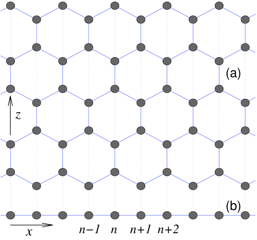
Figure 1: A scheme for constructing the chain model of the carbon nanoribbon. (a) Full-atomic model of GNR with zigzag orientation; (b) the chain model. Atomic rows of the nanoribbon oriented along the $z$-axis are numbered by the index $n$.

The chain model of GNR schematically shown in Fig. 2 can be described by the following Hamiltonian

$$H=\sum_{n=1}^{N}\frac{1}{2}M(\dot{x}^{2}_{n}+\dot{y}^{2}_{n})+\sum_{n=1}^{N-1}V(r_{n})$$

$$+\sum_{n=2}^{N-1}U(\theta_{n})+\sum_{n=1}^{N-4}\sum_{k=n+4}^{N}W_{i}(r_{nk}),$$ (1)

where $x_{n}$, $y_{n}$ are the coordinates of $n$-th particle, $r_{n}=|{\bf v}_{n}|$ is the distance between particles $n$ and $n+1$, with vector ${\bf v}_{n}=(x_{n+1}-x_{n},y_{n+1}-y_{n})$ connecting these particles, $\theta_{n}$ is the angle between vectors ${\bf v}_{n}$ and $-{\bf v}_{n-1}$, $r_{nk}$ is the distance between particles $n$ and $k$ (index $i=1$ if the difference $k-n$ is an odd number and $i=2$ if $k-n$ is an even number).

The first term in Eq. (1) gives the kinetic energy of the chain with $M=12m_{p}$ being the mass of carbon atom ($m_{p}=1.6603\cdot 10^{-27}$ kg is the proton mass) and the dot denotes differentiation with respect to time $t$. The harmonic potential

$$V(r)=\frac{1}{2}K(r-a)^{2},$$ (2)

describes the longitudinal stiffness of the chain.

The angular anharmonic potential in Eq. (1)

$$U(\theta)=\epsilon[\cos(\theta)+1],$$ (3)

stands for the flexural rigidity of the chain with $\cos(\theta_{n})=-({\bf v}_{n-1},{\bf v}_{n})/r_{n-1}r_{n}$ being the cosine of the $n$-th ”valent” angle.

The potential $W_{i}(r_{nk})$, $(i=1,2)$ in Eq. (1) describes the weak van der Waals interactions between particles $n$ and $k$, located at the distance $r_{nk}=\sqrt{(x_{k}-x_{n})^{2}+(y_{k}-y_{n})^{2}}$. These interactions, acting between nanoribbon layers, must be taken into account to describe folded or scrolled conformations of GNR. Without these interactions the only stable configuration of a nanoribbon is the flat one.

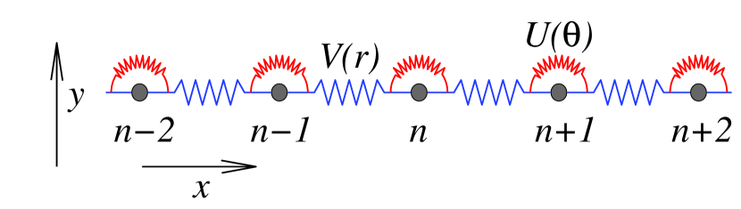
Figure 2: Chain of particles numbered by the index $n$ in the $xy$-plane, modeling tensile and bending motion of graphene nanoribbon. Potentials $V$ and $U$ describe the longitudinal and bending stiffness of the chain, respectively. The potential $W$ (not shown here) describes the weak van der Waals bonds acting between layers of the chain in the folded or rolled conformations.

Parameters of the Hamiltonian $K$ and $\epsilon$ are determined to fit the dispersion curves of the flat carbon nanoribbon presented in Fig. 1(a) to the dispersion curves of the straight chain model shown in Fig. 2. To do so, we consider dynamics of the flat nanoribbon, in line with the chain model, assuming that the atoms can move only in the $xy$-plane with all atoms in the rows along $z$-axis displaced equally. Let us denote the coordinates of the $n$-th atomic row as $x_{n}$ and $y_{n}$ and introduce the notation for the vector ${\bf u}_{n}=(x_{n},y_{n})$. For the flat nanoribbon the weak van der Waals interactions do not contribute to the dynamics and can be neglected. Then the Hamiltonian for the nanoribbon can be written in the form

$$H=\sum_{n=-\infty}^{+\infty}\left[\frac{1}{2}M(\dot{\bf u}_{n},\dot{\bf u}_{n})+P({\bf u}_{n-1},{\bf u}_{n},{\bf u}_{n+1},{\bf u}_{n+2})\right].$$ (4)

The first term in Eq. (4) describes the kinetic energy, while the second one stands for the potential energy of interatomic interactions, both per one carbon atom of $n$-th atomic row, located far from the nanoribbon edges. Thus, the effect of nanoribbon edges is not taken into account or, in other words, the nanoribbon width effect is not taken into account.

To describe the carbon-carbon valence interactions let us use a standard set of molecular dynamics potentials skh10prb . The valence bond between two neighboring carbon atoms $\alpha$ and $\beta$ can be described by the Morse potential

$$U_{1}({\bf u}_{\alpha},{\bf u}_{\beta})=\epsilon_{1}\{\exp[-\alpha_{0}(r-r_{0})]-1\}^{2},\,\,\,r=|{\bf u}_{\alpha}-{\bf u}_{\beta}|,$$ (5)

where $\epsilon_{1}=4.9632$ eV is the valence bond energy and $r_{0}=0.1418$ nm is the equilibrium valence bond length. Valence angle deformation energy between three adjacent carbon atoms $\alpha$, $\beta$, and $\gamma$ can be described by the potential

$$U_{2}({\bf u}_{\alpha},{\bf u}_{\beta},{\bf u}_{\gamma})=\epsilon_{2}(\cos\varphi-\cos\varphi_{0})^{2},$$ (6)

where $\cos\varphi=({\bf u}_{\gamma}-{\bf u}_{\beta},{\bf u}_{\alpha}-{\bf u}_{\beta})/(|{\bf u}_{\gamma}-{\bf u}_{\beta}|\cdot|{\bf u}_{\beta}-{\bf u}_{\alpha}|),$ and $\varphi_{0}=2\pi/3$ is the equilibrium valent angle. Parameters $\alpha_{0}=17.889$ nm^-1 and $\epsilon_{2}=1.3143$ eV can be found from the small amplitude oscillations spectrum of the graphene sheet sk08epl . Valence bonds between four adjacent carbon atoms $\alpha$, $\beta$, $\gamma$, and $\delta$ constitute torsion angles, the potential energy of which can be defined as

$$U_{3}(\phi)=\epsilon_{3}(1-\cos\phi),$$ (7)

where $\phi$ is the corresponding torsion angle ($\phi=0$ is the equilibrium value of the angle) and $\epsilon_{3}=0.499$ eV.

A detailed discussion of the choice of the interatomic potential parameters can be found in skh10prb . The same set of potentials has been successfully used to simulate the heat transfer along the carbon nanotubes and nanoribbons skh09epl ; shk09prb for the analysis of spatially localized oscillations sk94apl ; sk10epl ; sk10prb ; ksbdm12JETPLett ; kbd13epl ; bdz12epl and also for the investigation of theoretical strength and post-critical behavior of deformed graphene bdzs12prb ; dbsk11JETPLett ; bdsk12pss ; kd14jpd .

Hamiltonian Eq. (4) generates the following set of the equations of motion

$$-M\ddot{\bf u}_{n}=F_{1}({\bf u}_{n},{\bf u}_{n+1},{\bf u}_{n+2},{\bf u}_{n+3})$$

$$+F_{2}({\bf u}_{n-1},{\bf u}_{n},{\bf u}_{n+1},{\bf u}_{n+2})+F_{3}({\bf u}_{n-2},{\bf u}_{n-1},{\bf u}_{n},{\bf u}_{n+1})$$

$$+F_{4}({\bf u}_{n-3},{\bf u}_{n-2},{\bf u}_{n-1},{\bf u}_{n}),$$ (8)

where vector-function

$$F_{k}=\frac{\partial}{\partial{\bf u}_{k}}P({\bf u}_{1},{\bf u}_{2},{\bf u}_{3},{\bf u}_{4}),\leavevmode\nobreak\ \leavevmode\nobreak\ k=1,2,3,4.$$

It is convenient to use the relative coordinates of atoms ${\bf w}_{n}(t)={\bf u}_{n}(t)-{\bf u}_{n}^{0}$, where ${\bf u}_{n}^{0}$ are the equilibrium coordinates. For the analysis of small-amplitude vibrations ($|{\bf w}_{n}|\ll r_{0}$) we use the following linearized equations of motion

$$-M\ddot{\bf w}_{n}=B_{1}{\bf w}_{n}+B_{2}({\bf w}_{n-1}+{\bf w}_{n+1})$$

$$+B_{3}({\bf w}_{n-2}+{\bf w}_{n+2})+B_{4}({\bf w}_{n-3}+{\bf w}_{n+3}),$$ (9)

where matrices $B_{1}=F_{11}+F_{22}+F_{33}+F_{44}$, $B_{2}=F_{12}+F_{23}+F_{34}$, $B_{3}=F_{13}+F_{24}$, $B_{4}=F_{14}$, and matrix

$$F_{kl}=\frac{\partial}{\partial{\bf w}_{k}\partial{\bf w}_{l}}P({\bf 0},{\bf 0},{\bf 0},{\bf 0}).$$

We seek for the solution of linear system Eq. (9) in the form of the wave

$${\bf w}_{n}(t)={\bf A}\exp[i(qn-\omega t)],$$ (10)

where $\omega$ is the frequency of the wave, ${\bf A}$ is the amplitude vector, $q\in[0,\pi]$ is the dimensionless wavenumber. Substituting Eq. (10) into the linear system Eq. (9) we obtain the dispersion relation

$$|B_{1}+2\cos(q)B_{2}+2\cos(2q)B_{3}+2\cos(3q)B_{4}-\omega^{2}E|=0,$$ (11)

where $E$ is the unity matrix.

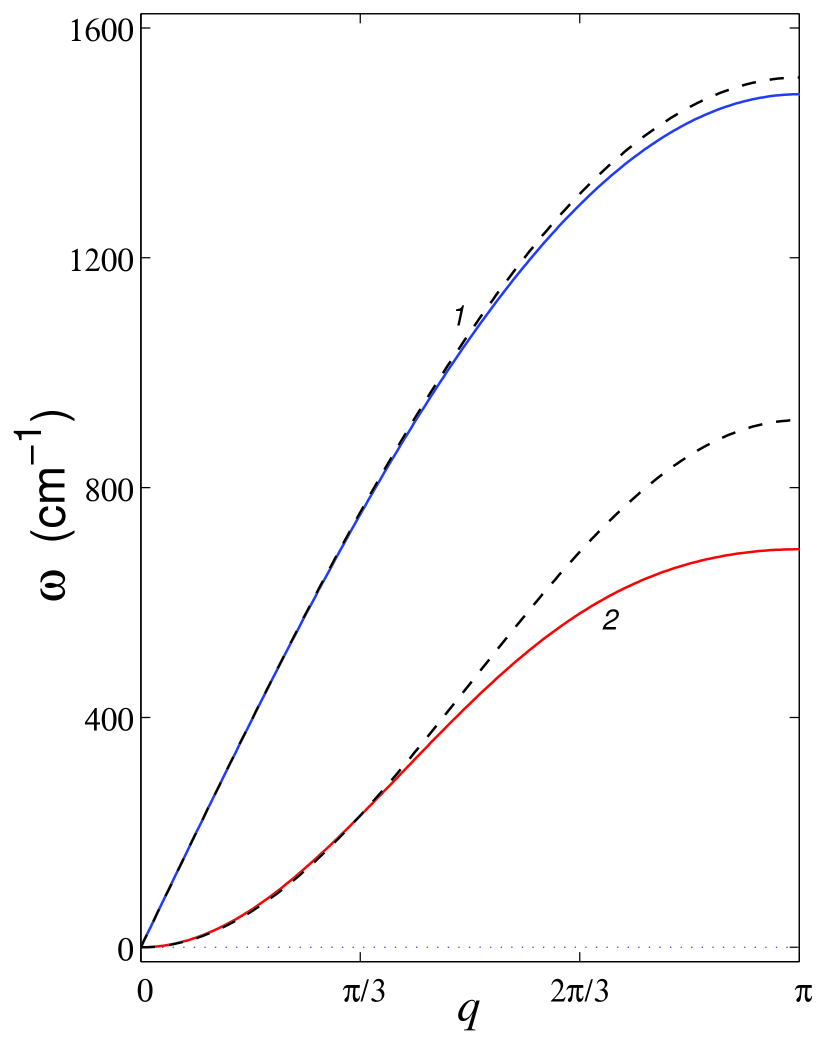
Figure 3: Dispersion curves of the wide carbon nanoribbon. Curve 1 stands for the longitudinal (tension-compression) and curve 2 for the transversal (bending) phonons. Solid lines correspond to the full-atomic model, while dashed lines to the chain model with appropriately chosen parameters.

The dispersion relation Eq. (11) is the second order polynomial with respect to the squared frequency $\omega^{2}$. The corresponding dispersion relation has two branches $0\leq\omega_{y}(q)\leq\omega_{x}(q)$ as plotted in Fig. 3 by the solid lines. The low-frequency branch $\omega=\omega_{y}(q)$ describes the dispersion of the transverse plane waves when lattice nodes leave the nanoribbon plane and move along $y$ axis (bending nanoribbon vibrations). The high-frequency branch $\omega=\omega_{z}(q)$ represents the dispersion of the longitudinal plane waves when the nodes move along $x$-axis (longitudinal nanoribbon vibrations).

Velocity of long-wavelength plane phonons coresponds to the velocity of sound which is

$$v_{x}=a\lim_{q\rightarrow 0}\omega_{x}(q)/q=17510\leavevmode\nobreak\ \mbox{m/s}$$

for the longitudinal phonons and

$$v_{y}=a\lim_{q\rightarrow 0}\omega_{y}(q)/q=0$$

for bending phonons.

Similarly, we can obtain the dispersion curves for the chain model. In this case, potential energy in the Hamiltonian Eq. (4) is defined as

$$P({\bf u}_{n-1},{\bf u}_{n},{\bf u}_{n+1})=V(r_{n})+U(\theta_{n}).$$

Potential parameters $K$ of Eq. (2) and $\epsilon$ of Eq. (3) should be chosen in a way to achieve the best fit of the dispersion curves obtained for the full-atomic model. We are interested in the long-wavelength modes of the nanoribbon motion and thus, the best fit should be achieved in the range of small values of $q$. The choice

$$K=405\leavevmode\nobreak\ \mbox{N/m},\leavevmode\nobreak\ \leavevmode\nobreak\ \leavevmode\nobreak\ \epsilon=3.50\leavevmode\nobreak\ \mbox{eV},$$ (12)

assures the coincidence of the longitudinal and flexural rigidity of the chain model and the nanoribbon, as can be seen in Fig. 3, where the result for the chain model is plotted by the dashed lines.

The van der Waals interactions between carbon atoms are described by the pairwise Lennard-Jones potential

$$W_{0}(r)=4\varepsilon[(\sigma/r)^{12}-(\sigma/r)^{6}],$$ (13)

where $r$ is the distance between two carbon atoms. The parameters of the Lennard-Jones potential $\varepsilon=0.002757$ eV and $\sigma=0.3393$ nm were fitted to reproduce the interlayer binding energy p22 , interlayer spacing p16 ; p17 , and $c$-axis compressibility p18 of graphite. The potential Eq. (13) with these parameters is shown in Fig. 4 by the curve 1.

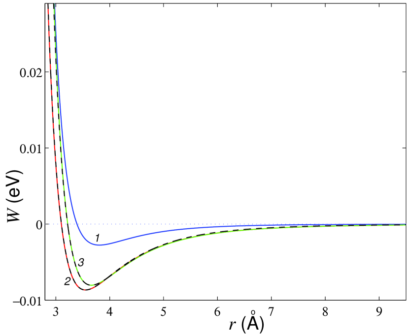
Figure 4: The pairwise Lennard-Jones potential $W_{0}(r)$ describing the van der Waals interaction between two carbon atoms (curve 1). Solid lines 2 and 3 show the potentials $W_{1}(r)$ and $W_{2}(r)$ (see in the text), while their approximation by the modified Lennard-Jones potentials Eq. (16) are shown by the dashed lines 2 and 3.

The long range interaction between the chain nodes $n$ and $k$ is described by the van der Waals interactions of the atoms belonging to $n$-th and $k$-th atomic row of the nanoribbon. Therefore, the interaction energy can be expressed as

$$W_{1}(r) = \sum_{j=-\infty}^{\infty}[W_{0}(r_{j,1})+W_{0}(r_{j,2})],$$

$$r_{j,1}=[r^{2}+(-0.5r_{0}+3jr_{0})^{2}]^{1/2},$$

$$r_{j,2}=[r^{2}+(-1.5r_{0}+3jr_{0})^{2}]^{1/2},$$

if the difference $k-n$ is an odd number and

$$W_{2}(r) = \sum_{j=-\infty}^{\infty}[W_{0}(r_{j,3})+W_{0}(r_{j,4})],$$

$$r_{j,3}=[r^{2}+(3jr_{0})^{2}]^{1/2},$$

$$r_{j,4}=[r^{2}+(-r_{0}+3jr_{0})^{2}]^{1/2},$$

if $k-n$ is an even number.

Interaction potentials Eq. (II) and Eq. (II) are well approximated by the modified Lennard-Jones potential

$$W_{i}(r)=4\varepsilon_{i}[(\sigma_{i}/f(r))^{12}-(\sigma_{i}/f(r))^{6}],$$

$$f(r)=r_{i}(r/r_{i})^{\alpha_{i}},\leavevmode\nobreak\ \leavevmode\nobreak\ \leavevmode\nobreak\ r_{i}=2^{1/6}\sigma_{i}.$$ (16)

For $i=1$, the modified potential parameters are $\varepsilon_{1}=0.008652$ eV, $\sigma_{1}=0.31636$ nm, and $\alpha_{1}=0.86$. For $i=2$, parameters are $\varepsilon_{2}=0.008029$ eV, $\sigma_{2}=0.32607$ nm, and $\alpha_{2}=0.90$. The interaction potentials of nanoribbon atomic rows Eq. (II) and Eq. (II) together with the corresponding modified Lennard-Jones approximations Eq. (16) are shown in Fig. 4 by the solid and dashed lines, respectively. Practically perfect coincidence of these potentials can be observed.

Summing up, for GNR shown in Fig. 1 (a), we have developed the chain model depicted in Fig. 2 and described by the Hamiltonian Eq. (1) with the parameters fitted to reproduce the long-wavelength phonon spectrum of GNR (see Fig. 3) and the van der Waals interactions acting between carbon atoms in folded or scrolled conformations of the nanoribbon (see Fig. 4). The chain model describes only such modes of GNR deformation in which the atomic rows parallel to $z$-axis move as rigid units only in the $xy$-plane but not in $z$-direction. The nanoribbon width effect is not taken into account.

III Secondary structures of single layer nanoribbon

To find stable structures of a one-layer carbon nanoribbon the following minimization problem should be considered

$$E=\sum_{n=1}^{N-1}V(r_{n})+\sum_{n=2}^{N-1}U(\theta_{n})$$

$$+\sum_{n=1}^{N-4}\sum_{k=n+4}^{N}W_{i}(r_{nk})\rightarrow\min:\{{\bf u}_{n}\}_{n=1}^{N},$$ (17)

where the minimization of potential energy of the chain model having $N$ nodes is performed with respect to the coordinates of the nodes ${\bf u}_{n}=(x_{n},y_{n})$, $n=1,2,...,N$. The nanoribbon length is defined by the number of nodes, $L=(N-1)a$.

The energy minimization was carried out numerically using the conjugate gradient method. In order to check the stability of the resulting stationary configuration $\{{\bf u}_{n}^{0}\}_{n=1}^{N}$ we calculate the eigenvalues of the $2N\times 2N$ matrix of the second derivatives

$$B=\left(\left.\frac{\partial E}{\partial u_{n,i}\partial u_{k,j}}\right|_{\{{\bf u}_{m}^{0}\}_{m=1}^{N}}\right)_{n=1,i=1,k=1,j=1}^{\leavevmode\nobreak\ \leavevmode\nobreak\ N,\leavevmode\nobreak\ \leavevmode\nobreak\ 2,\leavevmode\nobreak\ \leavevmode\nobreak\ N,\leavevmode\nobreak\ \leavevmode\nobreak\ 2}.$$ (18)

The stationary chain configuration is stable only if all eigenvalues of a symmetric matrix $B$ are non-negative: $\lambda_{i}\geq 0$, $i=1,2,...,2N$. Note that for stable configuration the first three eigenvalues are always zero $\lambda_{1}=\lambda_{2}=\lambda_{3}=0$. These eigenvalues correspond to the rigid motion of the chain in the $xy$-plane, with two translational and one rotational degrees of freedom. The remaining positive eigenvalues $\lambda_{i}>0$ correspond to the oscillation eigenmodes with frequencies $\omega_{i}=\sqrt{\lambda_{i}/M},\leavevmode\nobreak\ i=4,...,2N$.

Stationary structure of the chain depends on the initial configuration used to solve the minimization problem Eq. (17). Changing the initial configuration, a variety of stable configurations can be found. Linear chain configuration, representing flat nanoribbon, is always stable. The weak van der Waals interactions between nodes give rise to the existence of other, more advantageous in energy, stationary states of the chain in the two-dimensional space. As exemplified in Fig. 5, the chain consisting of $N=140$ nodes and having length $L=(N-1)a=17.070$ nm, in addition to the flat state, can be stable in (a) rolled, (b) double-folded, (c) triple-folded, and (d) rolled-collapsed conformations. Potential energy per node, $E_{0}=E/N$, is used to compare the energy of different chain conformations. In case of $N=140$, the flat structure has $E_{0}=-0.00453$ eV. For the other forms one has: $E_{0}=-0.01395$ eV for the rolled state, $-0.01214$ eV for the double-folded, $-0.00352$ eV for the triple-folded, and $-0.00662$ eV for the rolled-collapsed state. To understand these figures, one should keep in mind that formation of van der Waals bonds lowers the structure total energy, while the large curvature regions increase the energy. The rolled packing is the most energetically favorable among the studied conformations of the nanoribbon. All the studied non-flat structures have energy lower than the flat one, except for the triple-folded one. This is explained by the fact that the triple-folded structure possesses two loops with large curvature having no van der Waals bonds, and such loops have relatively large energy.

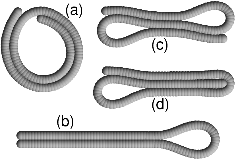
Figure 5: Stable stationary conformations of the chain model with $N=140$ nodes representing the nanoribbon of length $L=17.070$ nm: (a) rolled, (b) double-folded, (c) triple-folded, and (d) rolled-collapsed. Not shown here is the straight stable configuration (flat nanoribbon).

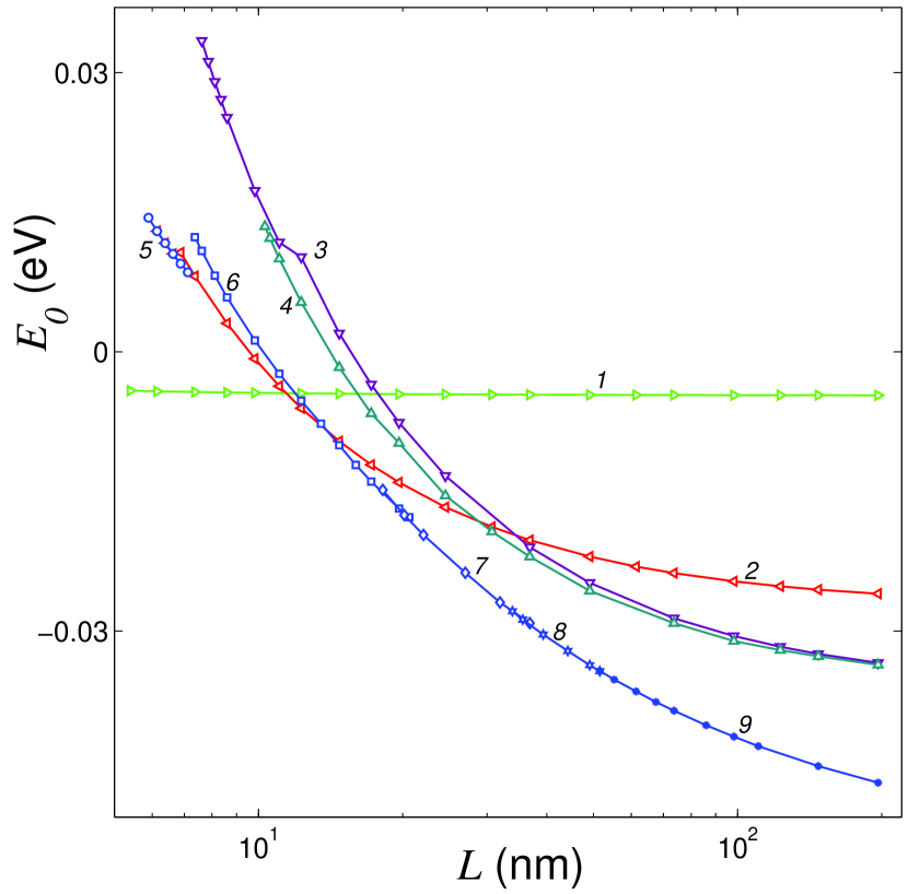
Figure 6: Potential energy per node, $E_{0}=E/N$, as the function of the chain length $L$ for flat nanoribbon (curve 1), double-folded (curve 2), triple-folded (curve 3), rolled-collapsed (curve 4), and for the rolled structures with one-coil (curve 5), two-coil (curve 6), three coil (curve 7), four coil (curve 8) and more coiled (curve 9) structures of the nanoribbon.

The dependence of the normalized energy $E_{0}$ for different stationary nanoribbon packages on its length $L$ is shown in Fig. 6. In the range $L<5.77$ nm the planar structure is the only stable configuration of the nanoribbon. For $L\geq 5.77$ nm, stable rolled structures exist. Chains with $L\geq 6.02$ nm ($L\geq 10.19$ nm) can support stable double-folded (triple-folded) structures. The rolled-collapsed structure requires the chain length $L\geq 10.19$ nm.

The flat nanoribbon has the lowest energy for $L<10.93$ nm. For the nanoribbon length in the range $10.93\leq L<13.39$ nm the lowest energy is observed for the double-folded configuration and for $L\geq 13.39$ nm the most energetically favorable is the rolled structure (nanoribbon scroll).

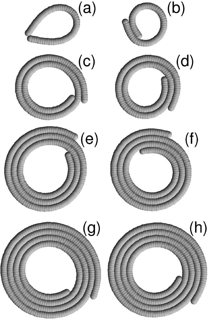
Figure 7: Examples of the stable, equilibrium scroll structures of the nanoribbon: (a) single coil scroll (nanoribbon length $L=7.00$ nm, energy per node $E_{0}=0.00881$ eV, number of coils $N_{c}=0.96$, inner and outer radii $R_{1}=R_{2}=1.11$ nm); (b) double coil scroll ($L=7.25$ nm, $E_{0}=0.0123$ eV, $N_{c}=1.19$, $R_{1}=0.97$ nm, $R_{2}=1.021$ nm); (c) double coil scroll ($L=19.53$ nm, $E_{0}=-0.01684$ eV, $N_{c}=1.98$, $R_{1}=1.40$ nm, $R_{2}=1.73$ nm); (d) three coil scroll ($L=19.53$ nm, $E_{0}=-0.01692$ eV, $N_{c}=2.19$, $R_{1}=1.24$ nm, $R_{2}=1.63$ nm); (e) three coil scroll ($L=34.26$ nm, $E_{0}=-0.02815$ eV, $N_{c}=2.96$, $R_{1}=1.51$ nm, $R_{2}=2.17$ nm); (f) four coil scroll ($L=34.26$ nm, $E_{0}=-0.02816$ eV, $N_{c}=3.14$, $R_{1}=1.38$ nm, $R_{2}=2.10$ nm); (g) four coil scroll ($L=51.45$ nm, $E_{0}=-0.03432$ eV, $N_{c}=3.94$, $R_{1}=1.58$ nm, $R_{2}=2.57$ nm); (h) five coil scroll ($L=51.45$ nm, $E_{0}=-0.03429$ eV, $N_{c}=4.05$, $R_{1}=1.51$ nm, $R_{2}=2.54$ nm).

IV Graphene nanoribbon scrolls

In the preceding Section it was shown that GNR having length $L\geq 13.39$ nm have the lowest energy in the rolled conformation among the other studied configurations. That is why, here we focus on the study of nanoribbon scrolls. The cross-sectional view of the minimum energy scroll structures for nanoribbons of increasing length can be seen in Fig. 7. The scroll cross-section appears in the form of the truncated Archimedes spiral always having inner cavity. The scroll structure is determined by the balance of energy gain caused by increasing the number of atoms having van der Waals bonds with the others and the energy loss due to the increase of nanoribbon curvature.

The center of mass can be considered as the center of the scroll:

$${\bf u}_{0}=\frac{1}{N}\sum_{n=1}^{N}{\bf u}_{n}^{0},$$

where ${\bf u}_{n}^{0}=(x_{n}^{0},y_{n}^{0})$ is the two-dimensional radius-vectors of the $n$-th chain node of the equilibrium scroll. In the polar coordinate system it can be written as

$$x_{n}^{0}=x_{0}+R_{n}^{0}\cos(\phi_{n}^{0}),\leavevmode\nobreak\ \leavevmode\nobreak\ y_{n}^{0}=y_{0}+R_{n}^{0}\sin(\phi_{n}^{0}),$$ (19)

where $R_{n}^{0}=\sqrt{(x_{n}^{0}-x_{0})^{2}+(y_{n}^{0}-y_{0})^{2}}$ and the discrete angle $\phi_{n}^{0}$ monotonously increases with increasing node number $n=1,2,...,N$. The spiral can be characterized by the number of coils

$$N_{c}=(\phi_{N}-\phi_{1})/2\pi.$$

It is also convenient to define the integer number of coils $m=[N_{c}]+1$, where $[x]$ is the integer part of $x$. Let us define the inner radius of scroll by its first coil:

$$R_{1}=\frac{1}{n_{1}}\sum_{n=1}^{n_{1}}R_{n}^{0},$$

where $n_{1}$ is the maximal value of index $n$ wherein $\phi_{n}<\phi_{1}+2\pi$. The outer radius of the scroll can be defined by its last coil as:

$$R_{2}=\frac{1}{N-n_{2}+1}\sum_{n=N-n2}^{N}R_{n}^{0},$$

where $n_{2}$ is the minimal value of $n$ where $\phi_{n}>\phi_{N}-2\pi$.

The twisting rigidity of the scroll is characterized by the lowest natural frequency $\omega_{1}=\sqrt{\lambda_{4}/M}$. This frequency corresponds to the periodic twisting/untwisting oscillations of the scroll. In the approximation of a continuous elastic rod this oscillation motion has been studied in spcg09apl ; spg10amss .

Figure 8: (a) Effect of the nanoribbon length $L$ on (a) the number of coils of the stationary scroll $N_{c}$, (b) inner $R_{1}$ (lower curve) and outer $R_{2}$ (upper curve) radii of the scroll, (c) the lowest natural vibration frequencies of the scroll, $\omega_{1}$ and $\omega_{2}$. The curves 1, 2, and 3 correspond to a single-coil scroll; curves 4-7 to the two-coil scroll; 8-11 to the three-coil scroll; 12-15 to four-coil scroll; curves 16-19 to the case of five and more layered structure of the nanoribbon scroll. The dashed lines are the fitting curves: (a) $N_{c}=0.33L^{0.63}$, (b) $R_{1}=0.67L^{0.2}$, $R_{2}=0.4L^{0.47}$, and (c) $\omega_{1}=36/L$, with $L$, $R_{1}$, and $R_{2}$ given in nanometers.

Let us describe how the scroll structure and the lowest natural frequency depend on the chain length (see Fig. 7 and Fig. 8). Various conformations can be naturally characterized by the number of coils $N_{c}$, energy per node $E_{0}$, inner and outer radii $R_{1}$, $R_{2}$.

Single-coil configuration is the only possible in the chain length range $5.772\leq L\leq 7.000$ nm [Fig. 7 (a)]. Double coil configuration is stable in case of $7.245\leq L\leq 20.508$ nm [Fig. 7 (b), (c)]. The chain length range $18.052\leq L\leq 36.718$ nm corresponds to stable three coil scrolls [Fig. 7 (d), (e)]. For the case of $33.771\leq L\leq 51.542$ nm the four-coiled scrolls are observed [Fig. 7 (f), (g)]. If nanoribbon length $L\geq 51.0$ nm, the scrolls with five or more coils exist [Fig. 7 (h)].

One can see that for nanoribbons with the same length two stable configurations are possible. For example, in the length range $18.052\leq L\leq 20.508$ nm stable two or three coil scrolls exist [Fig. 7 (c) and (d)]. Nanoribbons of length $33.771\leq L\leq 36.718$ nm can be packed in three or four coil scrolls [Fig. 7 (e) and (f)]. The reason for bistability is the result of the interaction of the nanoribbon ends. One stable configuration is when the ends are close to each other and another one is for somewhat overlapped ends. The degree of overlapping decreases with increasing nanoribbon length, as it can be seen in Fig. 7. Increase of the chain length leads to weakening of the interaction between ends and thus to weakening of the bistability of the scroll packing.

Increase in the nanoribbon length $L$ results in the monotonous increase in the number of coils $N_{c}$ according to the power law $N_{c}\approx 0.33L^{0.63}$, see Fig. 8 (a). The inner scroll radius $R_{1}$ increases much slower with $L$ than the outer radius $R_{2}$: $R_{1}\approx 0.67L^{0.2}$, $R_{2}\approx 0.4L^{0.47}$, see Fig. 8 (b). Here $L$, $R_{1}$, and $R_{2}$ are given in nanometers.

The eigenmode having lowest positive frequency $\omega_{1}$ is the twisting-untwisting mode when the atoms move along the Archimedes spiral. The second and the third lowest eigenfrequencies correspond to lateral compression-extension of the scroll. The scroll symmetry is lowered by the nanoribbon ends and for this reason the lateral compression in the two orthogonal directions is characterized by the close (but not equal) frequencies $\omega_{2}$ and $\omega_{3}$. These frequencies depend on $L$ nonmonotonically, see Fig. 8 (c). For $\omega_{1}$ the general trend is the reduction of the frequency with the growth in $L$ according to the law $\omega_{1}\approx 36/L$ for $L\rightarrow\infty$. This is in line with the asymptotic behavior obtained analytically in Refs. spcg09apl ; spg10amss .

V Frequency spectrum of the nanoribbon and nanoribbon scroll

Let us perform the full-atomic three-dimensional modeling of the dynamics of the nanoribbon scrolls to verify the two-dimensional chain model.

Let the set of two dimensional vectors $\{{\bf u}_{n}^{0}=(u_{n,1}^{0},u_{n,2}^{0})\}_{n=1}^{N}$ is the solution of the minimization problem Eq. (17), describing a scroll packing of the nanoribbon of length $L_{x}=(N-1)a$. For the nanoribbon of width $L_{z}=3Kr_{0}$ (the translational cell consist of $4K$ carbon atoms), then the coordinates of the atoms in $n$-th cell are

$$x_{n,4(k-1)+1} = u_{2n-1,1}^{0},\leavevmode\nobreak\ y_{n,4(k-1)+1}=u_{2n-1,2}^{0},$$

$$z_{n,4(k-1)+1} = 3(k-1)r_{0},$$

$$x_{n,4(k-1)+2} = u_{2n,1}^{0},\leavevmode\nobreak\ \leavevmode\nobreak\ \leavevmode\nobreak\ \leavevmode\nobreak\ y_{n,4(k-1)+2}=u_{2n,2}^{0},$$

$$z_{n,4(k-1)+1} = r_{0}/2+3(k-1)r_{0},$$

$$x_{n,4(k-1)+3} = u_{2n,1}^{0},\leavevmode\nobreak\ \leavevmode\nobreak\ \leavevmode\nobreak\ \leavevmode\nobreak\ y_{n,4(k-1)+3}=u_{2n,2}^{0},$$ (20)

$$z_{n,4(k-1)+1} = 3r_{0}/2+3(k-1)r_{0},$$

$$x_{n,4(k-1)+4} = u_{2n-1,1}^{0},\leavevmode\nobreak\ y_{n,4(k-1)+4}=u_{2n-1,2}^{0},$$

$$z_{n,4(k-1)+1} = 2r_{0}+3(k-1)r_{0},$$

$$k = 1,2,...,K,\leavevmode\nobreak\ \leavevmode\nobreak\ n=1,2,...,N/2,$$

where, as above, $r_{0}$ is equilibrium C-C valence bond length. In the case of odd number of cells, $N$, the nanoribbon consists of $N_{\rm all}=2NK$ carbon atoms. The two dimensional chain model and the full-atomic nanoribbon scroll are presented in Fig. 9 for the nanoribbon length $L_{x}=36.84$ nm and width $L_{z}=2.55$ nm ($N=301$, $K=6$, number of atoms $N_{all}=2NK=3612$).

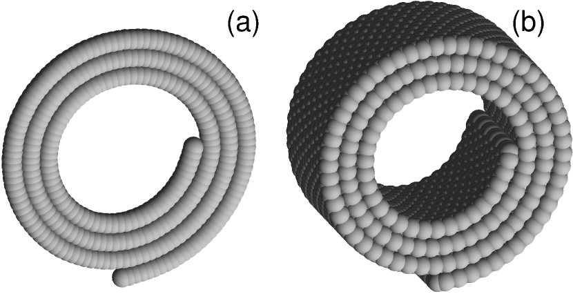
Figure 9: (a) Two dimensional chain model and (b) corresponding three dimensional full-atomic model of the nanoribbon scroll with the nanoribbon length $L_{x}=36.84$ nm and width $L_{z}=2.55$ nm ($N=301$, $K=6$, number of atoms $N_{\rm all}=2NK=3612$).

A set of interaction potentials (5), (6), (7), (13) was used for modeling of the nanoribbon dynamics. Valence bonds between neighboring atoms in the graphene plane are described by the Morse potential (5), valence and torsional angles by the potentials (6) and (7). Weak van der Waals interactions between scroll coils are described by the Lennard-Jones potential (13). Let us consider the edge carbon atoms chemically modified by hydrogen atoms and thus, having mass of $M_{0}=13m_{p}$, under the assumption that the interaction potentials for edge and internal atoms are the same.

Dynamics of the nanoribbon having size $L_{x}=(N-1)a\times 3Kr_{0}$ is described by the Langevin equations

$$M_{n,l}\ddot{\bf u}_{n,l}=-\frac{\partial H}{\partial{\bf u}_{n,l}}-\Gamma M_{n,l}\dot{\bf u}_{n,l}+\Xi_{n,l},$$ (21)

$$n=1,2,...,N,\leavevmode\nobreak\ \leavevmode\nobreak\ l=1,2,...,4K,$$

where ${\bf u}_{n,l}=(x_{n,l},y_{n,l},z_{n,l})$ is the three dimensional radius-vector of $(n,l)$-th atom, $M_{n,l}$ is the atom mass ($M_{n,l}=12m_{p}$ for the internal atoms and $M_{n,l}=13m_{p}$ for the edge atoms). Here $H$ is the nanoribbon Hamiltonian, $\Gamma=1/t_{r}$ is the friction coefficient, (velocity relaxation time is $t_{r}=0.4$ ps), random forces vectors $\Xi_{n,l}=(\xi_{n,l,1},\xi_{n,l,2},\xi_{n,l,3})$ are normalized as follows

$$\langle\xi_{n,l,i}(t_{1})\xi_{m,k,j}(t_{2})\rangle=2Mk_{B}T\delta_{nm}\delta_{lk}\delta_{ij}\delta(t_{1}-t_{2}).$$

The set of equations of motion Eq. (21) is integrated numerically. Initial conditions corresponding to the stationary scroll packing of the two-dimensional chain model Eq. (20) were used. We took $K=6$ and $N=101$, 201, 301, and 401 to simulate the nanoribbon of width $L_{z}=3Kr_{0}=2.5524$ nm and length $L_{x}=(N-1)a=12.28$, 24.56, 36.84, 49.12 nm. Numerical simulation at low temperature $T=3$ K has shown the absence of any noticeable changes in the initial structure of the scroll, i.e. the stationary configuration of the three dimensional scroll is well described by the equilibrium configuration of the two-dimensional chain. This confirms the high accuracy of the two-dimensional chain model.

In order to find the phonon density of states for the full-atomic flat nanoribbon and for the full-atomic scroll, the Langevin equations Eq. (21) were integrated for $10$ ps to achieve the state of thermal equilibrium at the desired temperature, and then the thermostat was switched off and free dynamics of atoms was studied. It was demonstrated numerically that the flat and scrolled nanoribbons of length $L_{x}=36.84$ nm are both stable in the temperature range $0\leq T\leq 900$ K. The use of full-atomic model allows us to find the time dependence of the particle velocity on time $\dot{\bf u}_{n,l}(t)$ and then the density of phonon states $p(\omega)$ normalized such that $\int_{0}^{\infty}p(\omega)d\omega=1$. The density of phonon states was determined from 600 homogenously distributed atoms and 256 independent realizations of the initial thermalized nanoribbon state in order to increase the calculation accuracy. The result for the nanoribbon of length $L_{x}=36.84$ nm and width $L_{z}=2.55$ nm is shown in Fig. 10 for the flat nanoribbon (red curves 1 and 3) and for the scroll (blue curves 2 and 4) at temperatures (a) $T=300$K and (b) $T=900$K. As one can see, the frequency spectra of the flat and scrolled nanoribbons are very close. Certain difference can be observed only in the low $\omega<150$ cm^-1 and high $\omega>1450$ cm^-1 frequency intervals. In the range $\omega<50$ cm^-1 the scroll has phonon density more than two times smaller than the flat nanoribbon. This is due to the fact that the rigidity of scroll is higher than that of nanoribbon and the low-frequency bending and torsional vibration modes are absent in the scroll. At high frequencies a small blue shift (by 5 cm^-1) of the oscillation frequencies is observed for the scroll. Scrolling of the nanoribbon leads to a moderate increase of oscillations frequencies in the range $\omega>1450$ cm^-1 due to the van der Waals interactions of atoms belonging to adjacent layers of the scroll.

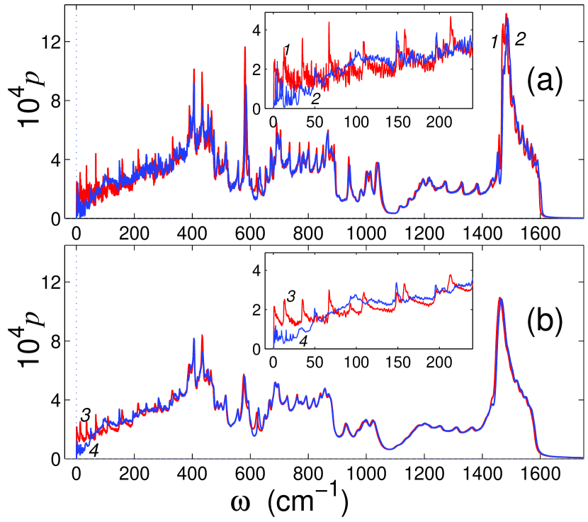
Figure 10: Phonon density of states $p(\omega)$ calculated from thermal vibrations of atoms for the flat nanoribbon (red curves 1 and 3) and for the scroll (blue curves 2 and 4) at temperatures (a) $T=300$K and (b) $T=900$K. The nanoribbon length and width are $L_{x}=36.84$ nm and $L_{z}=2.55$ nm, respectively.

VI Thermal expansion of scrolls

The scroll structure is stabilized by the weak van der Waals bonds acting between coils. Thermal fluctuations weaken such bonding leading to partial untwisting or full opening of the scroll. Fully opened scroll transforms to the flat GNR, while partial untwisting results in a reduction of the number of coils and in a growth of the scroll diameter.

The full-atomic model does not allow to simulate the long-term dynamics of wide multi-coiled nanoribbon scrolls due to the computer capacity limitations. For example, thermal expansion of the scroll can hardly be treated by the full-atomic model and this problem is addressed here in frame of the two-dimensional chain model.

For the simulation of thermal vibrations of the chain the Langevin equations were used

$$M\ddot{\bf u}_{n}=-\frac{\partial H}{\partial{\bf u}_{n}}-\Gamma M\dot{\bf u}_{n}+\Xi_{n},$$ (22)

$$n=1,2,...,N,$$

where ${\bf u}_{n}=(x_{n},y_{n})$ is the radius-vector of $n$-th node, $H$ is the Hamiltonian of the chain Eq. (1), $N$ is the number of nodes in the chain, $\Gamma=1/t_{r}$ is the friction coefficient (velocity relaxation time is $t_{r}=5$ ps), and $\Xi_{n}=(\xi_{n,1},\xi_{n,2})$ is the two dimensional vector of normally distributed random forces, normalized as

$$\langle\xi_{n,i}(t_{1})\xi_{m,j}(t_{2})\rangle=2Mk_{B}T\delta_{nm}\delta_{ij}\delta(t_{1}-t_{2})$$

(here $k_{B}$ is the Boltzmann constant).

The set of equations of motion Eq. (22) was integrated numerically. The stationary state of the scroll was used as an initial configuration.

Thermal stability of the scroll depends on the nanoribbon length $L$. The longer is the nanoribbon the larger is the energy of van der Waals bonds per atom and the higher is the thermostability. From simulations, it was found that single-coiled scroll of the nanoribbon having $L=(N-1)a=12.28$ nm (number of nodes $N=101$) is stable only for $T\leq 330$K and at higher temperatures it fully opens in less than $t=10$ ns. The two-coil scroll with $L=24.56$ nm $(N=201)$ was found to be stable within the whole studied temperature range $T\leq 960$K. Only partial untwisting is observed for the scrolls with this and higher values of $L$ in this temperature range.

Let us take the scroll of the nanoribbon of length $L=110.40$ nm (number of nodes $N=900$) for the study of its dynamics in the range of temperature $30\leq T\leq 960$K. The dependence of number of coils $N_{c}$ and inner and outer radii $R_{1}$, $R_{2}$ of the scroll on time is shown in Fig. 11. As one can see from the graph, thermal vibrations lead to decrease of the number of coils $N_{c}$ and growth of the radii $R_{1}$ and $R_{2}$.

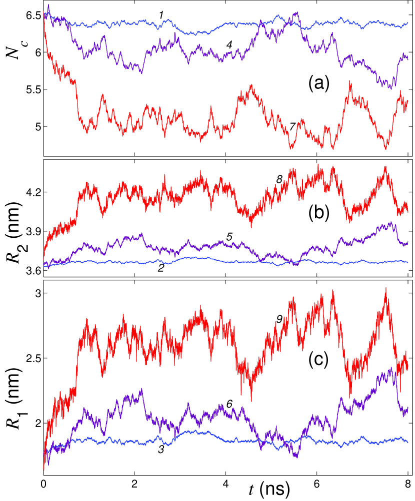
Figure 11: Time evolution of (a) number of coils $N_{c}$, (b) outer radius $R_{2}$, and (c) inner radius $R_{1}$ for the scroll of the nanoribbon having length $L=110.40$ nm, evaluated at the temperatures $T=30$ K (curves 1, 2, and 3), $T=300$ K (curves 4, 5, and 6), and $T=900$ K (curves 7, 8, and 9).

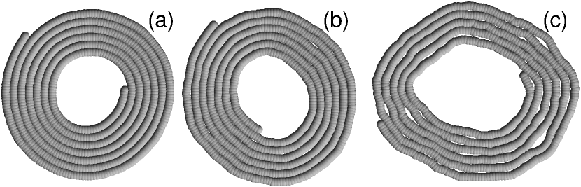
Figure 12: Typical scroll configurations for the nanoribbon having length $L=110.40$ nm (number of chain nodes $N$= 900) at temperatures (a) $T=30$K, (b) $T=300$K, and (c) $T=900$K.

Typical scroll configurations at different temperatures are shown in Fig. 12. At elevated temperatures the spiral structure is maintained and the inner and outer radii of the scroll increase with temperature.

In about 1 ns thermalization of scroll is complete and it obtains its equilibrium configuration. Further integration of the equations of atomic motion allows to determine the averaged values of the coil number $\bar{N}_{c}$ and inner and outer radii of the scroll, $\bar{R}_{1}$ and $\bar{R_{2}}$, corresponding to the given temperature. This values, as the functions of temperature, are plotted in Fig. 13. It can be seen that the number of coils decreases linearly, while the radii demonstrate a linear increase with temperature as $\bar{N}_{c}(T)\approx 6.52-0.00142T$, $\bar{R}_{i}(T)\approx R_{i}^{0}+c_{1}T$, where $i=1,2$, $R_{1}^{0}=1.782$ nm, $R_{2}^{0}=3.63$ nm, $c_{1}=0.00075$ nm/K, and $c_{2}=0.00047$ nm/K. The relative increase in the outer radius of the scroll of the nanoribbon having length $L=110.40$ nm is $\bar{R}_{2}(T)/R_{2}^{0}\approx 1+cT$, where the coefficient of linear thermal expansion is equal to $c=c_{2}/R_{2}^{0}=1.3\cdot 10^{-4}$K^-1. It was found that $c$ depends on $L$ such that $c$ is higher for smaller $L$. For example, for $L=73.56$ nm one has $c=1.4\cdot 10^{-4}$K^-1; for $L=36.84$ nm $c=1.8\cdot 10^{-4}$K^-1; and for $L=25.56$ nm $c=3.7\cdot 10^{-4}$K^-1.

Note that the coefficient of linear thermal expansion calculated for the graphene scroll outer radius is two (one) orders of magnitude larger than that for graphite in $a$ ($c$) direction (see CTE and references therein reporting on the experimental data) and two orders of magnitude larger than that for diamond CTEdiamond .

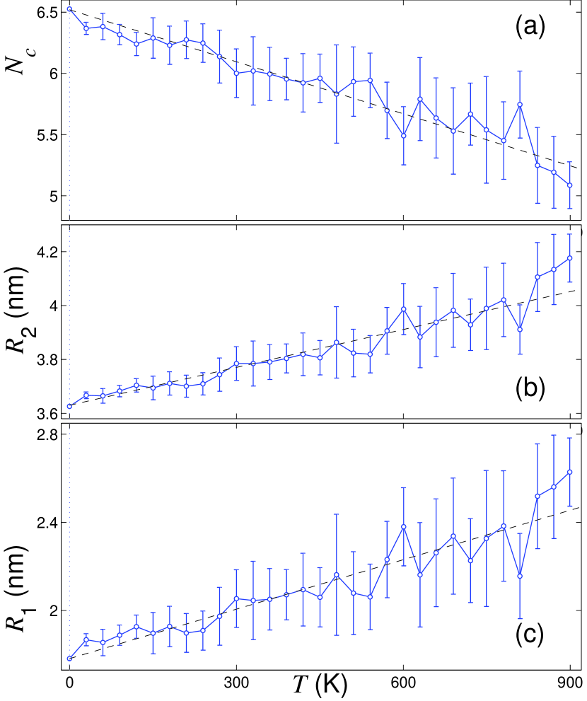
Figure 13: The temperature dependence of (a) the average number of coils $N_{c}$, (b) the outer radius $R_{2}$, and (c) the inner radius $R_{1}$ of the scroll of the nanoribbon having length $L=110.40$ nm. Dotted lines present the linear approximations.

VII Conclusions

In this paper, the two-dimensional chain model (see Fig. 2) was developed to accurately and effectively describe the dynamics of folded and rolled conformations of graphene nanoribbons. The Hamiltonian of the model is given by Eq. (1) and it takes into account the tensile and bending rigidity of the nanoribbon, as well as the van der Waals interactions between layers of the nanoribbon. The chain model describes only such modes of nanoribbon deformation [see Fig. 1 (a)], where the atomic rows parallel to $z$-axis move as rigid units only in the $xy$-plane but not in $z$-direction. The nanoribbon width effect is not taken into account. Parameters of the chain model were fitted to reproduce the low-frequency part of the phonon dispersion curves of the flat graphene nanoribbon (see Fig. 3). The van der Waals interactions were fitted by the modified Lennard-Jones potentials (see Fig. 4).

The validity of the chain model was demonstrated by comparison of the structure of the stationary nanoribbon scrolls with the results of full-atomic simulations.

Potential energy per atom was calculated for flat, rolled, double-folded, triple-folded, and rolled-collapsed conformations of nanoribbon as the function of its length $L$ (see Fig. 5 and Fig. 6). It was found that in the range $L<5.77$ nm the planar structure is the only stable configuration of the nanoribbon. For $L\geq 5.77$ nm, stable rolled structures exist. Chains with $L\geq 6.02$ nm ($L\geq 10.19$ nm) can support stable double-folded (triple-folded) structures. The rolled-collapsed structure requires the chain length $L\geq 10.19$ nm. The flat nanoribbon has the lowest energy for $L<10.93$ nm. For the nanoribbon length in the range $10.93\leq L<13.39$ nm the lowest energy is observed for the double-folded configuration, and for $L\geq 13.39$ nm the most energetically favorable is the rolled structure (nanoribbon scroll). These results can be easily interpreted in terms of the competition between energy release due to the formation of van der Waals bonds and energy absorption due to bending of the nanoribbon.

Since GNR having length $L\geq 13.39$ nm have the lowest energy in the rolled conformation among the other studied configurations, the nanoribbon scrolls were studied in detail (see Fig. 7 and Fig. 8). It was found that single-coil configuration is the only possible in the chain length range $5.772\leq L\leq 7.000$ nm. Double coil configuration is stable for $7.245\leq L\leq 20.508$ nm. The chain length range $18.052\leq L\leq 36.718$ nm corresponds to stable three coil scrolls. For the case of $33.771\leq L\leq 51.542$ nm the four-coiled scrolls are observed. For nanoribbon length $L\geq 51.0$ nm, the scrolls with five or more coils exist. Increase in the nanoribbon length $L$ results in the monotonous increase in the number of coils $N_{c}$ according to the power law $N_{c}\approx 0.33L^{0.63}$. The inner scroll radius $R_{1}$ increases much slower with $L$ than the outer radius $R_{2}$: $R_{1}\approx 0.67L^{0.2}$, $R_{2}\approx 0.4L^{0.47}$. Here $L$, $R_{1}$, and $R_{2}$ are given in nanometers. The twisting-untwisting eigenmode having lowest positive frequency $\omega_{1}$ was calculated as the function of nanoribbon length. For long nanoribbons the asymptotic law was found $\omega_{1}\approx 36/L$ for $L\rightarrow\infty$, which is in line with the earlier theoretical studies spcg09apl ; spg10amss .

Full-atomic model was used to calculate phonon density of states for flat and scrolled nanoribbons of length $L_{x}=36.84$ nm and width $L_{z}=2.55$ nm at 300 and 900 K (see Fig. 10). It was shown that the phonon spectra for the two conformations are very close in the entire frequency range. Small difference can be observed only in the low $\omega<150$ cm^-1 and high $\omega>1450$ cm^-1 frequency intervals. This can be explained by the higher rigidity of scroll due to formation of the van der Waals bonds between adjacent layers of the scroll. The low-frequency bending and torsional vibration modes are absent in the scroll.

One of the most important findings of the present study has emerged from the application of the developed chain model to the simulation of the long-term dynamics of nanoribbon scrolls at different temperatures. It was found that the relative increase in the outer radius of the scroll of the nanoribbon having length $L=110.40$ nm is characterised by the coefficient of linear thermal expansion of $c=1.3\cdot 10^{-4}$K^-1. It was found that $c$ depends on $L$ such that $c$ is higher for smaller $L$. For example, for $L=73.56$ nm one has $c=1.4\cdot 10^{-4}$K^-1; for $L=36.84$ nm $c=1.8\cdot 10^{-4}$K^-1; and for $L=25.56$ nm $c=3.7\cdot 10^{-4}$K^-1. The coefficient of linear thermal expansion calculated for the graphene scroll outer radius is two (one) orders of magnitude larger than that for graphite in $a$ ($c$) direction CTE and two orders of magnitude larger than that for diamond CTEdiamond . Such anomaly in the coefficient of thermal expansion can be used in the design of nanosensors or other nanodevices.

The developed planar chain model can help to address problems related to the dynamics of open graphene structures not treatable by the full-atomic simulations. The results obtained in frame of the chain model could provide a better understanding of the mechanical properties of CNS-based nanodevices.

VIII Acknowledgements

A.V. Savin thanks financial support provided by the Russian Science Foundation, grant N 14-13-00982, and the Joint Supercomputer Center of the Russian Academy of Sciences for the use of computer facilities. E.A. Korznikova is grateful for the financial support from the President Grant for young scientists (grant N MK-5283.2015.2). S.V. Dmitriev appreciates the support from the Tomsk State University Academic D.I. Mendeleev Fund Program.

References

- (1) K.S. Novoselov, A.K. Geim, S.V. Morozov, D. Jiang, Y. Zhang, S.V. Dubonos, I.V. Grigorieva, and A.A. Firsov, Science 306, 666 (2004).
- (2) A.K. Geim and K.S. Novoselov, Nat. Mater. 6, 183 (2007).
- (3) C. Soldano, A. Mahmood, and E.Dujardin, Carbon 48, 2127 (2010).
- (4) R. Won, Nat. Photonics 4, 411 (2010).
- (5) X. Li, H. Zhu, K. Wang, A. Cao, and J.Wei, Adv. Mater. 22, 2743 (2010).
- (6) W. Bollmann and J. Spreadborough, Nature, 186, 29 (1960).
- (7) L.M. Viculis, J.J. Mack, and R.B. Kaner, Science 299, 1361 (2003).
- (8) M.V. Savoskin, V.N. Mochalin, A.P. Yaroshenko, N.I. Lazareva, T.E. Konstantinova, I.V. Barsukov, and I.G. Prokofiev, Carbon 45, 2797 (2007).
- (9) D. Roy, E. Angeles-Tactay, R.J.C. Brown, S.J. Spencer, T. Fry, T.A. Dunton, T. Young, and M.J.T. Milton, Chem. Phys. Lett. 465, 254 (2008).
- (10) X. Xie, L. Ju, X. Feng, Y. Sun, R. Zhou, K. Liu, S. Fan, Q. Li, and K. Jiang, Nano Lett. 9, 2565 (2009).
- (11) A.L. Chuvilin, V.L. Kuznetsov, A.N. Obraztsov, Carbon 47, 3099 (2009).
- (12) G. Cheng, I. Calizo, X. Liang, B.A. Sperling, A.C. Johnston-Peck, W. Li, J.E. Maslar, C.A. Richtera, and A.R.H. Walker, Carbon 76, 257 (2014).
- (13) H.Q. Zhou, C.Y. Qiu, H.C. Yang, F. Yu, M.J. Chen, L.J. Hu, Y.J. Guo, and L.F. Sun, Chem. Phys. Lett. 501, 475 (2011).
- (14) X. Chen, R.A. Boulos, J.F. Dobson, and C.L. Raston, Nanoscale, 5, 498 (2013).
- (15) H. Pan, Y. Feng, and J. Lin, Phys. Rev. B 72, 085415 (2005).
- (16) R. Rurali, V. R. Coluci, and D. S. Galvao, Phys. Rev. B 74, 085414 (2006).
- (17) Y. Chen, J. Lu, and Z. Gao, J. Phys. Chem. C 111, 1625 (2007).
- (18) S.F. Braga, V.R. Coluci, S.B. Legoas, R. Giro, D.S. Galvao, and R.H. Baughman, Nano Lett. 4, 881 (2004).
- (19) X. Shi, N.M. Pugno, Y. Cheng, and H. Gao, J. Appl. Phys. 95, 163113 (2009).
- (20) B.V.C. Martins and D.S. Galvao, Nanotechnology 21, 075710 (2010).
- (21) S. Huang, B. Wang, M. Feng, X. Xu, X. Cao, and Y. Wang, Surf. Sci. 634, 3 (2015).
- (22) E. Perim, R. Paupitz, and D.S. Galvao, J. Appl. Phys. 113, 054306 (2013).
- (23) Y. Wang, H.F. Zhan, C. Yang, Y. Xiang, and Y.Y. Zhang, Comp. Mater. Sci 96 300 (2015).
- (24) X. Shi, Y. Cheng, N.M. Pugno, and H. Gao, J. Appl. Phys. 96, 053115 (2010).
- (25) Z. Zhang and T. Li, Appl. Phys. Lett. 97, 081909 (2010).
- (26) L. Chu, Q. Xue, T. Zhang, and C. Ling, J. Phys. Chem. C 115, 15217 (2011).
- (27) N. Patra, Y. Song, and P. Kral, ACS Nano 5, 1798 (2011).
- (28) H.Y. Song, S.F. Geng, M.R. An, and X.W. Zha, J. Appl. Phys. 113, 164305 (2013).
- (29) Q. Yin and X. Shi, Nanoscale 5, 5450 (2013).
- (30) X. Shi, N.M. Pugno, H. Gao, Acta Mech. Solida Sin. 23, 484 (2010).
- (31) X. Shi, N.M. Pugno, H. Gao, Int. J. Fract. 171, 163 (2011).
- (32) V.R. Coluci, S.F. Braga, R.H. Baughman, and D.S. Galvao, Phys. Rev. B 75, 125404 (2007).
- (33) S.F. Braga, V.R. Coluci, R.H. Baughman, D.S. Galvao, Chem. Phys. Lett. 441, 78 (2007).
- (34) X. Shi, Y. Cheng, N.M. Pugno, and H. Gao, Small 6, 739 (2010).
- (35) X. Shi, Q. Yin, N.M. Pugno, and H. Gao, J. Appl. Mech. 81, 1014 (2013).
- (36) Z. Zhang, Y. Huang, and T. Li, J. Appl. Phys. 112, 063515 (2012).
- (37) A.V. Savin, Y.S. Kivshar, and B. Hu, Phys. Rev. B 82, 195422 (2010).
- (38) A. V. Savin and Yu. S. Kivshar, Europhys. Lett. 82, 66002 (2008).
- (39) A.V. Savin, Y.S. Kivshar, and B. Hu, Europhys. Lett. 88, 26004 (2009).
- (40) A.V. Savin, B. Hu, and Y.S. Kivshar, Phys. Rev. B 80, 195423 (2009).
- (41) A.V. Savin and Y.S. Kivshar, Appl. Phys. Lett. 94, 111903 (2009).
- (42) A.V. Savin and Y.S. Kivshar, Europhys. Lett. 89, 46001 (2010).
- (43) A.V. Savin and Y.S. Kivshar, Phys. Rev. B 81, 165418 (2010).
- (44) E.A. Korznikova, A.V. Savin, Y.A. Baimova, S.V. Dmitriev, and R.R. Mulyukov, JETP Lett. 96, 222 (2012).
- (45) E.A. Korznikova, J.A. Baimova, and S.V. Dmitriev, Europhys. Lett. 102, 60004 (2013).
- (46) J.A. Baimova, S.V. Dmitriev, and K. Zhou, Europhys. Lett. 100, 36005 (2012).
- (47) J.A. Baimova, S.V. Dmitriev, K. Zhou, and A.V. Savin, Phys. Rev. B 86, 035427 (2012).
- (48) S.V. Dmitriev, Y.A. Baimova, A.V. Savin, and Y.S. Kivshar’, JETP Lett. 93, 571 (2011).
- (49) Y.A. Baimova, S.V. Dmitriev, A.V. Savin, and Y.S. Kivshar’, Phys. Solid State 54, 866 (2012).
- (50) E.A. Korznikova and S.V. Dmitriev, J. Phys. D: Appl. Phys. 47, 345307 (2014).
- (51) R. Zacharia, H. Ulbricht, and T. Hertel, Phys. Rev. B 69, 155406 (2004).
- (52) A. Ludsteck, Acta. Crystallogr. A 28, 59 (1972).
- (53) Y.X. Zhao and I.L. Spain, Phys. Rev. B 40, 993 (1989).
- (54) W.B. Gauster and I.J. Fritz, J. Appl. Phys. 45, 3309 (1974).
- (55) D.K.L. Tsang, B.J. Marsden, S.L. Fok, and G. Hall, Carbon 43, 2902 (2005).
- (56) S. Stoupin and Yu.V. Shvyd ko, Phys. Rev. Lett. 104, 085901 (2010).