A new approach for physiological time series

Abstract

We developed a new approach for the analysis of physiological time series. An iterative convolution filter is used to decompose the time series into various components. Statistics of these components are extracted as features to characterize the mechanisms underlying the time series. Motivated by the studies that show many normal physiological systems involve irregularity while the decrease of irregularity usually implies the abnormality, the statistics for “outliers” in the components are used as features measuring irregularity. Support vector machines are used to select the most relevant features that are able to differentiate the time series from normal and abnormal systems. This new approach is successfully used in the study of congestive heart failure by heart beat interval time series.

Key words: iterative convolution filter, outliers, support vector machines, congestive heart failure, heart beat intervals

1 Introduction

An understanding of physiological time series such as the heart-beat intervals is important to many areas, like heart-attack prediction, cardiovascular health, sport and exercise, etc. The study of time series can reveal underlying mechanisms of the physiological system, which usually contains both deterministic and stochastic components. Therefore the analysis of time series is very complicated because of the nonlinear and non-stationary characteristics of physiological time series data. Over the past years, time series analysis methods are applied to quantify physiological data for identification and classification (Kantz et al., 1998; Schreiber, 1999). The applications of physiological time series analysis commonly focus on measuring different aspects of time series data such as complexity, regularity, predictability, dimensionality, randomness, self similarity, etc. The tools used in these techniques include but not restrict to the mean, standard deviation, Fourier transform, wavelet, entropy, fractal dimension, pattern detection (Kantz and Schreiber, 1997; Tong, 1990).

Recently a new mathematical tool, empirical mode decomposition (EMD), was proposed by Norden Huang and his collaborators (Huang et al., 1998, 1999). It decomposes a time series into a finite sum of intrinsic mode functions (IMF) that generally admit well-behaved Hilbert transforms. This decomposition is based on the local characteristic time scale of the data, which makes EMD applicable to analyze nonlinear and non-stationary signals. EMD and Hilbert transform together, called the Hilbert-Huang transform (HHT), usually allow to construct meaningful time-frequency representations of signals using instantaneous frequency of the data. EMD and HHT have been applied with great success in many application areas such as biological and medical sciences, geology, astronomy, engineering, and others (Huang et al., 1998; Chen et al., 2006; Echeverria et al., 2001; Huang et al., 1999; Pines and Salvino, 2002; Liu et al., 2006). Another interesting set of examples is the work of L.Yang and his collaborators, who have successfully applied EMD based techniques for texture analysis and Chinese handwriting recognition (Yang et al., 2006b, a; Zheng et al., 2008).

The main purpose of this paper is to develop a new approach for the analysis of physiological times series. Our approach is motivated by two intuitions and coupled with modern machine learning techniques. The first intuition comes from a belief that a physiological system should contain a deterministic part that reflects the basic mechanism for the system to survive and a stochastic part that represents the variability of resilience. Mathematically they can be represented by the low frequency and high frequency components of a physiological signal. This motivates the application of methods of decomposing signals into various components according to frequencies in the quantitative analysis of physiological time series. Examples include the Fourier transform, wavelets, and EMD. In our method we will use an iterative convolution filter which is an alternative of EMD. The second intuition comes from a statistical perspective of irregularity. A lot of study has proved that normal physiological systems show irregularity due to the existence of stochastic components while the decrease of irregularity usually implies the abnormality. From statistical perspective, irregularity of a data set is represented by the “outliers”. This motivates us to study the statistics of outliers in physiological time series. However, we must be careful in doing so. Practical physiological times series usually contain noise which may also appear as outliers. We have to guarantee the “outliers” we examined are not pure noise. This is possible because true outliers do not have informative structures and could be detected. The second intuition is the motivation for our feature construction in Section 2.2.

These two intuitions enable us to decompose the physiological times series and construct features for our quantitative analysis. Combining with the well established feature selection techniques in machine learning we can remove the redundancy of the features and find relevant statistics for classification of physiological time series. Support vector machine recursive feature elimination(SVM-RFE) is suggested in this paper for linear classification problems. The details of our approach will be described in Section 2.

We will use our approach to analyze the heart beat interval time series and study the congestive heart failure problem. The study of heart diseases such as congestive heart failure by using heart beat interval times series has a long history. Decrease of heart rate variability or cardiac chaos has been found in congestive heart failure (Poon and Merrill, 1997; Casolo et al., 1989). In the literature, many methods and metrics have been proposed to analyze the difference between the heart rate times series of healthy people and congestive heart failure patients, to name a few, the detrended fluctuation analysis (Peng et al., 1995), multifractality (Ivanov et al., 1999), multiscaling entropy (Costa et al., 2005), hierarchical entropy (Jiang et al., 2011). Our approach is different from the methods in the literature. It incorporates advanced machine learning techniques and allows the data “to speak by itself.” By applying our approach, the purposes are two-fold: The first is to build good classifiers to enable good diagnosis. The second is to find what kind of irregularity is associated to the heart health. The results and discussions are summarized in Section 3.

The novelty of our method is mainly the following two points. Firstly, although we decompose the time series into components of different frequencies, we do not compare them from the frequency domain. Secondly, we proved that the outliers in a physiological time series are usually not pure noise but are informative instead. Interestingly, although this idea is motivated by physiological times series analysis, it is also found successful in the stylometry analysis of artworks (Hughes et al., 2012).

2 Method

2.1 Signal decomposition

Let $L$ be a low pass filter. Denote by $T$ the weak limit of the the operator $(I-L)^{n}$ as $n\to\infty$, i.e., for a discrete signal $X$ and time $t$

$$T(X)(t)=\lim_{n\to\infty}(I-L)^{n}(X)(t).$$

Using this operator iteratively, a signal $X$ can be decomposed as follows: Let $F_{1}=T(X)$ and for $k\geq 2$,

$$F_{k}=T\left(X-\sum_{i=1}^{k-1}F_{i}\right).$$

After $m$ steps we get $F_{1},\ldots,F_{m}$ which we call mode functions and the residual

$$R=X-\sum_{i=1}^{m}F_{i}.$$

Then we have

$$X=F_{1}+F_{2}+\ldots+F_{m}+R.$$

In this decomposition, roughly speaking the former mode functions are noise or high frequency components and the latter mode functions are low frequency components and $R$ is the trend.

This procedure follows the spirit of the traditional EMD introduced in Huang et al. (1998). In the traditional EMD, the low pass filter $L$ is chosen as the average of the upper envelope (the cubic spline connecting the local maxima) and the lower envelope (the cubic spline connecting the local minima). This method, although has been successfully used in many applications, is lack of theoretical foundation and has its limitations.

In Lin et al. (2009) a new approach is proposed. In this new approach the low pass filter is a moving average generated by a mask $\mathbf{a}=(a_{j})_{j=-N}^{N}$ that gives the $L(X)$ as the convolution of $a$ and $X$, i.e.,

$$L(X)(t)=\sum_{j=-N}^{N}a_{j}X(j+t).$$

With this choice of $L$ we call the operator $T$ an iterative convolution filter. A rigorous mathematical foundation and convergence analysis is given in Lin et al. (2009); Huang et al. (2009). Note the mask $\mathbf{a}$ is finitely supported on $[-N,N]$ and $N$ is called the window size. The flexibility to choose the window size is crucial in applications and forms a main advantage of this method.

Similar to decompositions by many other methods like Fourier transform and wavelets, the trend and low frequency components are usually assumed to characterize the profile of the signal and the high frequency components characterize the details. In different applications we need the features of difference components.

2.2 Feature extraction

After decomposing the signal into the mode functions and the trend, we need to extract statistics that can characterize the essential features of these components. This step requires a priori knowledge of the problem under consideration. It could be rather weak. But without any priori knowledge, it is difficult to get proper statistics. Also, this step is strongly problem dependent. In the following let us use the heart-beat intervals as an example to illustrate how to construct the features.

In this application, each time series is a record of heart beat intervals in 24 hours (Costa et al., 2005). It is first decomposed into several mode functions. To extract the features, for each mode function $F_{i},$ we first get its mean $m_{i}$ and standard deviation $\sigma_{i}$. By the previous studies (Poon and Merrill, 1997; Casolo et al., 1989; Costa et al., 2005) the healthy heart beats more irregularly than the unhealthy heart. This motivates us to design the statistics to measure the irregularity. To this end, we consider the terms that are larger than $m_{i}+\sigma_{i}$ and find their mean $m_{i,1}$ and standard deviation $\sigma_{i,1}$. We also find the mean $m_{i,2}$ and standard deviation $\sigma_{i,2}$ of the terms that are larger than $m_{i}+2\sigma_{i}$. Symmetrically we also get the mean $m_{i,-1}$ and standard deviation $\sigma_{i,-1}$ of those terms that are smaller than $m_{i}-\sigma_{i}$, and the mean $m_{i,-2}$ and standard deviation $\sigma_{i,-2}$ of those terms that are smaller than $m_{i}-2\sigma_{i}.$ This procedure gives us 10 statistics. Note all those terms that are outside the one or two standard deviations are in some sense “outliers” and it is natural to use their statistics ($m_{i,j}$ and $\sigma_{i,j}$ for $j=1,2,-1,-2$) to characterize the irregularity. Next we consider the times series $U_{i}$ composed of local maxima of $F_{i}$ and the time series $L_{i}$ composed of the local minima of $F_{i}$. These two series measure the local amplitude. For each series we compute the 10 statistics by the same procedure above as for $F_{i}$. Therefore for each mode function $F_{i}$ we get 30 statistics.

Unlike in (Costa et al., 2005), we use the whole 24-hour heart beat time series and assume we do not know the periods for different activities such as sleeping and walking. We think the statistics for different periods should be different and not all of them represent the difference between the healthy and unhealthy people. This motivates the idea of splitting the whole time series into subseries. Suppose we split the time series into $K$ subseries for each subject. Correspondingly we also split each mode function $F_{i}$ into $K$ subcomponents, which are denoted by $F_{i}^{k},\ k=1,\ldots,K.$ For each subcomponent $F_{i}^{k}$, we compute the 30 statistics as above: 10 for $F_{i}^{k}$ itself, 10 for the local maxima $U_{i}^{k},$ and 10 for the local minima $L_{i}^{k}.$ For each $i$ and each statistics, we have $K$ values from the $K$ subcomponents. We compute the mean, the first quartile (the 25th quantile), the third quartile (the 75th quantile) of these $K$ values to obtain 3 features. This gives 90 features. So for each model function $F_{i}$ we get 120 features in total.

For physiological signals, we believe the trend and low frequency components are determined by the fundamental mechanism while the individual differences should be reflected by the high frequency components. In case that we do not have much knowledge about the disease to be diagnosed we may assume the features may also come from the trend. So the same 120 statistics are also computed for the trend component.

To represent these features, we introduce the notations for the statistics and three subscripts to indicated how the statistics is calculated. The detailed descriptions are listed in Table 1.

Type	Notations or Values	Description
Statistics	$m$	mean of the time series
	$\sigma$	standard deviation of the time series
	$mm$	mean of subcomponent means
	$m\sigma$	mean of subcomponent standard deviations
	$qm$	1st quartile of subcomponents means
	$q\sigma$	1st quartile of subcomponent standard deviations
	$Qm$	3rd quartile of subcomponents means
	$Q\sigma$	3rd quartile of subcomponent standard deviations
Subscript 1	$i=1,2,\ldots,m$	Statistics computed from $F_{i}$.
	$i=R$	Statistics computed from $R$.
Subscript 2	$j=0$ or omitted	Statistics for the whole series or subseries.
	$j=+1$ or $+2$	Statistics for the terms greater than $m+j\sigma$.
	$j=-1$ or $-2$	Statistics for the terms less than $m-|j|\sigma$.
Subscript 3	$0$ or omitted	Statistics computed from $F_{i}$ or $R$.
	$L$	Statistics computed from local minima.
	$U$	Statistics computed from local maxima.

Table 1: The notations for the features.

2.3 Feature subset selection

After the above two steps we get a large number of features for the data. Usually only a small part of them are related to the diagnosis and the physiological mechanism of the disease. The task of the third step is to find the relevant ones. This will be realized by eliminating the irrelevant ones step by step.

Firstly, if a statistic is almost constant, then it is useless in the diagnosis and should be eliminated. For example, the means of the mode functions $m_{i}$ are all approximately zero and should be eliminated.

Next we use the SVM-RFE method (Guyon et al., 2002) to rank the features. In this method, given a set of training samples, we first train linear SVM to get a linear classifier and then rank the features according to the weights. Because of large feature size and small training samples, the classifier might not be as good. Also, the high correlation between the features may result the relevant features to have small weights. These reasons could lead the rank to be inaccurate. In order to refine the rank we eliminate the least important feature and repeat the process to re-rank the remained features. Running this process iteratively we finally get the refined rank of the features.

With this rank of features we can conclude which statistics are useful for the diagnosis and characterize the essence of the underlying physiological mechanism. Good classifiers can then be built to make accurate diagnosis.

3 Experiments and Results

In this section we apply our new method described above to the heart beat interval times series and report our results and conclusions.

3.1 The data set

The data set includes the heart beat interval time series of 72 healthy people and 43 CHF patients. For each subject the heart beat interval is measured for 24 hours under various activities. In our experiment we will assume the activity period is not known. The CHF of $43$ patients are classified into 4 degrees where the degree I is a slight CHF and the degree IV is a severe CHF. Most CHF patients are of the degree III.

3.2 A primary study

Before using our new method, we study the classification ability of two simple statistics: mean and variance. In Figure 1 we plot the mean and variance of the heart beat intervals for the healthy people and CHF patients. We see that the healthy people and the CHF patients can be roughly separated. The average heart beat interval of healthy people is larger and so is the variance. It shows the heart of healthy people beats slower and more irregularly. This observation is consistent with the previous studies.

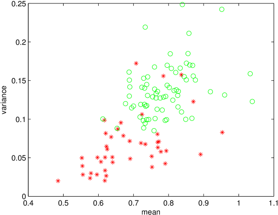
Figure 1: The mean and variance (in second) of heart beat interval times series, ‘o’ for healthy subjects and ‘*’ for CHF patients.

At the same time, we notice that several CHF patients falling into the cluster of healthy people show to be severe CHF patients. So we conjecture that the mean and variance might not reflect the essence of the underlying mechanism, although they have good separability.

3.3 Experiment: feature extraction

For each time series, we use the iterative convolution filter to realize the signal decomposition. In this step we need to specify the window size of the mask. It turns out it should be chosen between 50 and 100 to be stable. In our experiment it is chosen to be $50.$

We then calculate the statistics proposed in Section 2.2. Here we need to specify the parameter $K$, the number of subseries. If a statistic really captures the essence of the data set, it should be stable and independent of the choice of $K$ once it is chosen within a reasonable interval. Our experiments show that $K=50$ is a good choice. Most heart beat signals were recorded for a little bit more than 24 hours. Thus when $K=50$, each subseries is around 30 minutes of record.

Previous studies have shown that healthy heart beats irregularly. In statistics, irregularity could be measured by statistics of “outliers” that are not due to noise. This motivates us to consider the statistics of upward and downward fluctuations. At the same time, from the study in Section 3.2 we find that a healthy heart beats slower than an unhealthy heart in average. These two intuitions enlighten us to conjecture that those larger heart beat intervals (i.e. slower heart beats) in the time series characterize the difference between the healthy people and CHF patients. To confirm this, we do a correlation analysis.

For each of the first two mode functions and each $j=1,2,-1,-2$, we calculate and sort the means $m_{ij}^{k}$ and standard deviations $\sigma_{ij}^{k}$ for the $K=50$ subcomponents. For each order statistics we compute its correlation to the CHF disease. The result is plotted in Figure 2. From the comparison we see that, in average, correlations of the statistics associated to upward fluctuations are larger than those associated to downward fluctuations. This observation tells that we may disregard the statistics for the downward fluctuations.

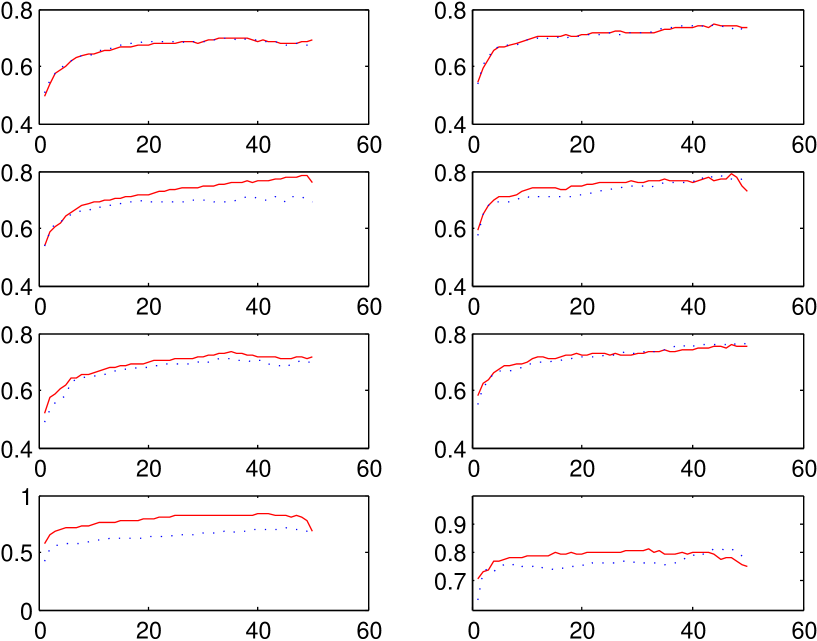
Figure 2: The correlations of various statistics to the CHF disease. The first column is for the first mode function $F_{1}$ and the second column is for the second mode function $F_{2}$. The first row is for order statistics of $m_{i,1}^{k}$ (red solid line) versus the order statistics of $m_{i,-1}^{k}$ (blue dotted line). The second row is for order statistics of $\sigma_{i,1}^{k}$ (red solid line) versus the order statistics of $\sigma_{i,-1}^{k}$ (blue dotted line). The third row is for order statistics of $m_{i,2}^{k}$ (red solid line) versus the order statistics of $m_{i,-2}^{k}$ (blue dotted line). The last row is for order statistics of $\sigma_{i,2}^{k}$ (red solid line) versus the order statistics of $\sigma_{i,-2}^{k}$ (blue dotted line).

3.4 Feature ranking and subset selection

To rank the features, we randomly split the data set into two subsets as the training set and the test set, respectively. In the training set we have 50 healthy subjects and 30 CHF subjects and in the test set there are 22 healthy and 13 CHF subjects. We use the training set to build the SVM classifier and use the test set to control the accuracy. Using the SVM-RFE methods described in Subsection 2.3 we rank the features. To guarantee the stability of the rank we repeat this procedure 1000 times and choose the statistics that appear most frequently in the model.

In all 1000 repeats, the classification error on the test data set is summarized in the following table:

number of errors	0	1	2	3	4	5
number of repeats	823	116	42	14	4	1

Table 2: Number of errors and the corresponding number of repeats.

The top 10 features selected by the procedure are listed in Table 3. We see 9 of them are related to the first two IMFs. Although the trend is in general not considered relevant, the last feature, associated to the trend, appears. We suspect a probable reason is that using only two mode functions in the signal decomposition leaves some relevant information in the trend. It is interesting to notice that these 10 statistics that appear most frequently in the model all measure the irregularity of the local amplitude. Take Statistics 1 and Statistics 7 as the example. They are obtained as the following. To get Statistics 1, for the first mode function $F_{1}$, find the local maxima $U_{1}$ and compute its mean $m_{1,0,U}$ and the standard deviation $\sigma_{1,0,U}$. Then we choose terms greater than $m_{1,0,U}+2\sigma_{1,0,U}$ and find their standard deviation. To get Statistics 7, for the subcomponents of the second mode function, $F_{2}^{k},k=1,\ldots,K$, compute the mean $m_{2}^{k}$ and the standard deviation $\sigma_{2}^{k}$. Then we choose terms greater than $m_{2}^{k}+2\sigma_{2}^{k}$ of $F_{2}^{k}$ and find their standard deviations $\sigma_{2,2}^{k}.$ Then we compute the mean of $K$ such standard deviations. In Figure 3 we show the distribution of the healthy people and CHF patients using these two statistics. It is easy to see that healthy people and CHF patients are well separated.

Feature Rank	1	2	3	4	5
Statistics	$\sigma_{1,2,U}$	$\sigma_{1,-2,U}$	$m\sigma_{1,2}$	$m\sigma_{1,2,U}$	$m\sigma_{1,2,L}$
Feature Rank	6	7	8	9	10
Statistics	$\sigma_{2,2}$	$m\sigma_{2,2}$	$m\sigma_{2,2,U}$	$m\sigma_{2,-2,L}$	$m\sigma_{R,1,U}$

Table 3: The top 10 features.

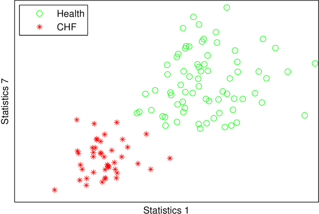
Figure 3: Distribution of CHF patients vs healthy subjects using Statistics 1 ($\sigma_{1,2,U}$) and Statistics 7 ($m\sigma_{2,2}$).

Observing these two statistics, we find that both of them measure the ability of the heart beat to become extremely slower than usual. It leads to the conjecture that the strong adaptability of extremely slower heart beat might be the irregularity that characterizes the healthy hearts.

3.5 Reliability of the top features

We have found that the most relevant features are statistics for the “outliers” in the mode functions, i.e., those items larger than mean plus two times standard deviations, or items less than mean minus two times standard deviations. A natural question arises: “Is this accidental?” This is equivalent to ask whether the outliers taken into account are noise or informative.

In order to answer this question we further analyze these outliers. Firstly we notice that the up and down fluctuations are not balanced for both healthy people and CHF patients. The percentage of items larger than mean plus two times standard deviation for healthy people is 2.84% and those items smaller than the mean minus two stand deviation is only 2.35%. For CHF patients the percentages are 2.49% and 2.17%, respectively. This observation is the first evidence that outliers are not due to noise because otherwise they should be balanced distributed. Moreover, recall for Gaussian white noise the percentage of one-side outliers outside the two times standard deviation is 2.28%. We see the outliers for CHF is closer to it while those for healthy subjects are much larger. We think that the outliers for CHF patients involve more noise while the outliers for healthy subjects are probably informative.

To further confirm our conclusion, we do the following test: for $F_{1}$, we calculate the statistics for the terms greater than the mean plus $v$ times standard deviation with the variable $v$ changing from 0 to 2 and investigate their correlation to the CHF disease. Here we consider mean of the 50 standard deviations of such terms in the 50 subcomponents. Note Statistics 3 in Table 3 corresponds to $v=2.$ The correlation is plotted in Figure 4. From this analysis, we see the correlation increases with $v$. Such a trend appears also in other statistics. This clear trend implies that the relevancy between these statistics and the CHF disease is not accidental. Instead, we should consider the outliers informative and their properties characterize the essence difference between healthy people and CHF patients.

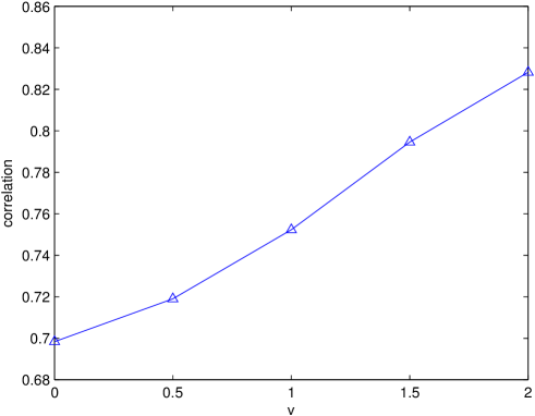
Figure 4: Correlations between CHF disease and the mean of the 50 standard deviations of those terms greater than the mean plus $v$ times standard deviation in the 50 subcomponents. The value of $v$ varies from 0 to 2.

4 Conclusions and discussions

In this paper we developed a new approach for the analysis of the physiological times series. The motivation comes from that the physiological times series usually contains both deterministic and stochastic parts and they can be represented by the low and high frequency components of the times series. Our new method uses an iterative filter to realize the decomposition of the times series into high and low frequency components and study their statistics. SVM-RFE is then used to select highly relevant features.

Our method is applied to analyze the heart beat interval time series for CHF disease. The top features are found to measure the ability of hearts to beat extremely slowly. Healthy hearts show strong ability which we conjecture is due to the strong resilience to the environment and human activities.

References

- Casolo et al. [1989] G. Casolo, E. Balli, T. Taddei, J. Amuhasi, and C. Gori. Decreased spontaneous heart rate variability in congestive heart failure. The American journal of cardiology, 64(18):1162–1167, 1989.
- Chen et al. [2006] Q. Chen, N. Huang, S. Riemenschneider, and Y. Xu. A B-spline approach for empirical mode decompositions. Adv. Comput. Math., 24(1-4):171–195, 2006.
- Costa et al. [2005] M. Costa, A. L. Goldberger, and C.-K. Peng. Multiscalce entropy analysis of biological signals. Physical Review, E, 71:021906, 2005.
- Echeverria et al. [2001] J. Echeverria, J. Crowe, M. Woolfson, and B. Hayes-Gill. Application of empirical mode decomposition to heart rate variability analysis. Medical and Biological Engineering and Computing, 39:471–479, 2001.
- Guyon et al. [2002] I. Guyon, J. Weston, S. Barnhill, and V. Vapnik. Gene selection for cancer classification using support vector machines. Machine Learning, 46:389–422, 2002.
- Huang et al. [2009] C. Huang, L. Yang, and Y. Wang. Convergence of a convolution-filtering-based algorithm for empirical mode decomposition. Advances in Adaptive Data Analysis, 1(04):561–571, 2009.
- Huang et al. [1998] N. E. Huang, Z. Shen, S. R. Long, M. C. Wu, H. H. Shih, Q. Zheng, N. Yen, C. Tung, and H. H. Liu. The empirical mode decomposition and the Hilbert spectrum for nonlinear and non-stationary time series analysis. Proceedings of the Royal Society of London, A, 454:903–995, 1998.
- Huang et al. [1999] N. E. Huang, Z. Shen, and S. R. Long. A new view of nonlinear water waves: the Hilbert spectrum. In Annual review of fluid mechanics, Vol. 31, pages 417–457. Annual Reviews, Palo Alto, CA, 1999.
- Hughes et al. [2012] J. M. Hughes, D. Mao, D. N. Rockmore, Y. Wang, and Q. Wu. Empirical mode decomposition analysis for visual stylometry. Pattern Analysis and Machine Intelligence, IEEE Transactions on, 34(11):2147–2157, 2012.
- Ivanov et al. [1999] P. C. Ivanov, L. A. N. Amaral, A. L. Goldberger, S. Havlin, M. G. Rosenblum, Z. R. Struzik, and H. E. Stanley. Multifractality in human heartbeat dynamics. Nature, 399(6735):461–465, 1999.
- Jiang et al. [2011] Y. Jiang, C.-K. Peng, and Y. Xu. Hierarchical entropy analysis for biological signals. Journal of Computational and Applied Mathematics, 236(5):728–742, 2011.
- Kantz and Schreiber [1997] H. Kantz and T. Schreiber. Nonlinear time series analysis, volume 7 of Cambridge Nonlinear Science Series. Cambridge University Press, Cambridge, 1997.
- Kantz et al. [1998] H. Kantz, J. Kurths, and G. Mayer-Kress. Nonlinear techniques in physiological time series analysis. Springer series in synergetics. Springer, Heidelberg, 1998.
- Lin et al. [2009] L. Lin, Y. Wang, and H. Zhou. Iterative filtering as an alternative algorithm for empirical mode decomposition. Advances in Adaptive Data Analysis, 1(04):543–560, 2009.
- Liu et al. [2006] B. Liu, S. Riemenschneider, and Y. Xu. Gearbox fault diagnosis using empirical mode decomposition and Hilbert spectrum. Mechanical Systems and Signal Processing, 20(3):718–734, 2006.
- Peng et al. [1995] C.-K. Peng, S. Havlin, H. E. Stanley, and A. L. Goldberger. Quantification of scaling exponents and crossover phenomena in nonstationary heartbeat time series. Chaos: An Interdisciplinary Journal of Nonlinear Science, 5(1):82–87, 1995.
- Pines and Salvino [2002] D. Pines and L. Salvino. Health monitoring of one dimensional structures using empirical mode decomposition and the Hilbert-Huang transform. In Proceedings of SPIE, volume 4701, pages 127–143, 2002.
- Poon and Merrill [1997] C.-S. Poon and C. K. Merrill. Decrease of cardiac chaos in congestive heart failure. Nature, 389(6650):492–495, 1997.
- Schreiber [1999] T. Schreiber. Interdisciplinary application of nonlinear time series methods. Phys. Rep., 308(2), 1999.
- Tong [1990] H. Tong. Nonlinear Time Series Analysis. Oxford University Press, Oxford, 1990.
- Yang et al. [2006a] Z. Yang, L. Yang, and D. Qi. Detection of spindles in sleep EEGs using a novel algorithm based on the Hilbert-Huang transform. In T. Qian, M. I. Vai, and Y. Xu, editors, Wavelet Analysis and Applications, Applied and Numerical Harmonic Analysis, pages 543–559. Birkhauser, 2006a.
- Yang et al. [2006b] Z. Yang, L. Yang, D. Qi, and C. Suen. An EMD-based recognition method for Chinese fonts and styles. Pattern Recognition Letter, 27:1692–1701, 2006b.
- Zheng et al. [2008] T. Zheng, L. Xie, and L. Yang. Integrated extraction on handwritten numeral strings in form document based on hybrid binarization. Pattern Recognition and Artificial Intelligence, 21(3):369–375, 2008.