GARROTXA cosmological simulations of Milky Way-sized galaxies: General properties, hot gas distribution and missing baryons

Abstract

We introduce a new set of simulations of Milky Way-sized galaxies using the AMR code ART + hydrodynamics in a $\Lambda$CDM cosmogony. The simulation series is named GARROTXA and follow the formation of a halo/galaxy from z $=$ 60 to z $=$ 0. The final virial mass of the system is $\sim$7.4$\times$10¹¹M_⊙. Our results are as follows: (a) contrary to many previous studies, the circular velocity curve shows no central peak and overall agrees with recent MW observations. (b) Other quantities, such as M$\_{*}$(6$\times$10¹⁰M_⊙) and R_d (2.56 kpc), fall well inside the observational MW range. (c) We measure the disk-to-total ratio kinematically and find that D/T=0.42. (d) The cold gas fraction and star formation rate (SFR) at z=0, on the other hand, fall short from the values estimated for the Milky Way.
As a first scientific exploitation of the simulation series, we study the spatial distribution of the hot X-ray luminous gas. We have found that most of this X-ray emitting gas is in a halo-like distribution accounting for an important fraction but not all of the missing baryons. An important amount of hot gas is also present in filaments. In all our models there is not a massive disk-like hot gas distribution dominating the column density. Our analysis of hot gas mock observations reveals that the homogeneity assumption leads to an overestimation of the total mass by factors 3 to 5 or to an underestimation by factors $0.7-0.1$, depending on the used observational method. Finally, we confirm a clear correlation between the total hot gas mass and the dark matter halo mass of galactic systems.

1. Introduction

One of the most challenging problems that hydrodynamical simulations have faced since the pioneering works of Evrard (1988); Hernquist & Katz (1989); Cen et al. (1990); Navarro & Benz (1991); Navarro & White (1993) has been to produce, within the standard $\Lambda$CDM hierarchical structure formation scenario, systems that look like real disk galaxies; that is, galaxies with extended disks and present-day star formation rates, disk-to-bulge ratios, and gas and baryonic fractions that agree with observations.

It has been long known that disks should form when gas cools and condenses within dark matter halos (White & Rees, 1978; Fall & Efstathiou, 1980; Mo et al., 1998) conserving angular momentum obtained through external torques from neighbouring structures (Hoyle, 1953; Peebles, 1969). Yet, the first halo/galaxy hydrodynamical simulations (Navarro & Benz, 1991; Navarro & Steinmetz, 2000) inevitably ended up with small and compact disks and massive spheroids that dominated the mass. Two effects were found to be the responsible of this result. First, artificial losses of angular momentum caused by insufficient resolution and other numerical effects (Abadi et al., 2003; Okamoto et al., 2003; Governato et al., 2004; Kaufmann et al., 2007). Second, the dynamical friction that transfers the orbital angular momentum of merging substructures to the outer halo and causes cold baryons (stars plus gas) to sink to the center of the proto-galaxy (e.g. Hernquist & Mihos, 1995). Once in the center, baryons that are still in the form of gas are quickly converted to stars. These newborn stars will join the stellar component and both will form an old spheroid, leaving no gas for the formation of new disk stars at latter times (e.g. Maller & Dekel, 2002). Later, the increase in resolution in the numerical simulations led to several authors (e.g. Robertson et al., 2004; Okamoto et al., 2005; Governato et al., 2004) to succeed in getting more realistic disk galaxies. This better resolution was achieved using the so called zoom-in technique. This technique allows simulators to obtain high resolution by choosing a small region, almost always a sphere centered on a specific halo, from a relatively big box, and rerun it with higher resolution (e.g. Klypin et al., 2001). To obtain a “MW-like” system the authors selected halos with masses similar to the one estimated for the MW ($\sim$10¹² M _⊙) and halos that have not suffered a major merger since $z$ $\sim$ 1.5 (e.g. Robertson et al., 2004; Governato et al., 2004; Okamoto et al., 2005; Scannapieco et al., 2009; Guedes et al., 2011; Moster et al., 2014; Vogelsberger et al., 2014).

The recent relative success on forming more realistic disk galaxies has not been limited to resolution. The implementation of new subgrid physics such as an efficient supernovae (SNe) feedback (Stinson et al., 2006) and new star formation recipes have shown to be important (Gnedin et al., 2009). The more effective stellar feedback acts by removing low-angular-momentum material from the central part of (proto)galaxies (e.g. Brook et al., 2012) while a SF based on the molecular hydrogen abundance is more realistic. These improvements make simulated galaxies to follow observed scaling relations, like the Tully-Fisher, for the first time (Governato et al., 2007) and thus relax the tension that existed between observations and $\Lambda$CDM predictions (Governato et al., 2010). In galaxy formation simulations, gas is accreted in filamentary cold flows that never is shock-heated to the halo virial temperature (Kereš et al., 2005; Dekel et al., 2009). This cold gas is the fuel for the late star formation in disks (Kereš et al., 2009; Ceverino et al., 2010). For instance, authors like Scannapieco et al. (2009); Stinson et al. (2010); Piontek & Steinmetz (2011); Agertz et al. (2011); Brooks et al. (2011); Feldmann et al. (2011); Guedes et al. (2011) obtained realistic rotationally supported disks with some properties closely resembling the MW ones.

Until recently, simulated disk galaxies with rotation curves similar to that of the Milky Way were scarce. Most works used to obtain systems with too peaked and declining rotation curves (e.g. Scannapieco et al., 2012; Hummels & Bryan, 2012). Agertz et al. (2011) showed that by fine tuning the values of the SF efficiency and the gas density SF threshold parameters it was possible to avoid the formation of galaxies with such peaked rotation curves. In more recent high resolution simulations, including ours, this is not longer a problem (Aumer et al., 2013; Mollitor et al., 2015; Marinacci et al., 2014; Murante et al., 2015; Agertz & Kravtsov, 2015; Keller et al., 2015; Santos-Santos et al., 2016), in part due to an added “early-feedback” (Stinson et al., 2013) to the thermal SNe one, the implementation of an efficient kinetic feedback, and/or the inclusion of the AGN feedback. The early feedback is attributed to a feedback that is present from the very beginning, before the first supernova explodes, and it may include radiation pressure (Krumholz, 2015), photoheating of the gas due to the ionizing radiation of massive stars (Trujillo-Gomez et al., 2015), stellar winds, etc. Currently the need of such effects are widely acknowledged but their correct implementations are still a challenge (Oman et al., 2015; González-Samaniego et al., 2014).

Obtaining systems that resemble the MW open several possibilities on the study of galaxy formation and evolution. For instance, it is interesting to study the origin of the galactic halo coronal gas, their properties and how they can account for a fraction of the missing baryons. The lack of baryons in the universe was reported by Fukugita et al. (1998) when they found that cosmological baryon fraction inferred from Big Bang nucleosynthesis is much higher than the one obtained by counting baryons at redshift z = 0. This problem was confirmed when a more accurate value for the cosmological baryon fraction was obtained from the high precision data of WMAP (Dunkley et al., 2009) and Planck (Planck Collaboration et al., 2014). In fact, the cosmic ratio $\Omega_{b}$/$\Omega_{M}$ is 3$-$10 times larger than the one observed for galaxies. To solve this missing baryons problem, following the natural prediction from structure formation models (White & Rees, 1978; White & Frenk, 1991), authors like Cen & Ostriker (1999); Davé et al. (2001); Bregman (2007) proposed that galactic winds, SNe feedback or strong AGN winds ejected part of the galactic baryons to the dark matter halo and circumgalactic medium (CGM) as hot gas. Others authors like Mo & Mao (2004) proposed that also part of the gas never collapsed into the dark matter halos as it was previously heated by SNe of Population III. From the point of view of large volume hydrodynamical galaxy formation simulations, some attempts have been made in order to investigate the presence and detectability of hot gas halo corona. Toft et al. (2002) presented one of the first studies towards this direction, however due to the inefficient feedback, the amount of hot gas in their simulated halo was too small. Global properties of hot gas halo corona in MW-sized simulations have also been studied (e.g. Guedes et al., 2011; Mollitor et al., 2015). More recently, models that account for the SNe feedback and implement new star formation processes, succeeded in obtaining more realistic results when compared with observations (Crain et al., 2010, 2013).

From an observational point of view the hot gas halo corona was proposed to be detected by its X-ray emission. First detections where done by Forman et al. (1985) in external galaxies and later on several authors get better detections in other systems and studied them deeper (e.g. Mathews & Brighenti, 2003; Li et al., 2008; Anderson & Bregman, 2010; Bogdán & Gilfanov, 2011). More recently, using Chandra, XMM-Newton, FUSE and other instruments (e.g. Hagihara et al., 2010, 2011; Miller & Bregman, 2013a) it was detected a large reservoir of this hot gas surrounding our galaxy (e.g. $\sim$6$\times$10¹⁰ M _⊙ in Gupta et al., 2012) and it was proposed that it could account for a fraction of the so called missing baryons mass. These detections were done by the analysis of X-ray absorption lines from OVII and OVIII which only exist in environments with temperatures between 10⁶ and 10⁷ K, the MW halo has a temperature of about $log$ T = 6.1$-$6.4 (Yao & Wang, 2007; Hagihara et al., 2010). The problem of using this technique is that these X-ray absorption lines only can be observed in the directions of extragalactic luminous sources (QSO, AGN, …) or galactic X-ray emitters as X-ray binaries. This observational strategy gives a limited information about hot gas distribution and position, inside the galactic halo or in the intergalactic medium. Using this limited information, several recent works (Gupta et al., 2012; Miller & Bregman, 2013b; Gupta et al., 2014) obtained a value for the total hot gas mass embedded in the galactic halo that accounts for about 10$-$50$\%$ of missing baryons. To obtain these total hot gas mass from the low number of available observations the authors needed to assume a simple hot gas density profile. It is important to be aware that this assumption can lead to biased total hot gas mass values. Recently Faerman et al. (2016) used an analytic phenomenological model to study the warm/hot gaseous coronae distribution in galaxies. They have used the MW hot gas X-ray and UV observations as input for their model and found that the warm/hot halo coronae may contain a large reservoir of gas. They conclude that if metallicity is of about 0.5 solar it can account for an important fraction of the missing baryons.

Here, we introduce a new set of MW-sized simulations with a high number of DM particles and cells ($\sim$7$\times$10⁶). On the other hand, the spatial resolution, the side of the cell in the maximum level of refinement, is 109 pc. These are highly resolved simulations even for today standards. The simulated galaxy ends up with an extended disk and an unpeaked slowly decreasing rotation curve. It is important to mention that the subgrid physics used in the present work was shown to produce realistic low-mass galaxies, at least as far as the rotation curves was concerned (e.g. Colín et al., 2013). In the GARROTXA series of simulations the temperature reached by the gas in the cells, where stellar particles are born, is actually higher than the one obtained in, for example, the simulations by González-Samaniego et al. (2014) because the SF efficiency factor is higher (0.65 versus 0.5). This along with the fact that here the gas density threshold is lower, 1 cm ^-3 instead of 6 cm ^-3, makes the stellar feedback in GARROTXA simulations stronger.
Using our simulations we have also studied how the hot gas component embedded in the DM halo can account for part of the missing baryons in galaxies. A novelty of the present paper is the determination, in our GARROTXA series of simulations, of the hot halo gas distribution in a full sky view which offers us an opportunity to detect observational biases in the determination of its mass, when only a small number of line of sight observations are used.

This paper is laid out as follows. In Sec. 2 we present the code and initial conditions we have used. In Sec. 3 we introduce the general properties of our MW-sized simulations, whilst in Sec. 4 we present the study of their hot gas component. We summarize our conclusions in Sec. 5.

2. GARROTXA simulation

2.1. The code

The numerical simulations we introduce in this work (GARROTXA: GAlaxy high Resolution Runs in a cOsmological ConteXt using ART) have been computed using the Eulerian hydrodynamics + N-body ART code (Kravtsov et al., 1997; Kravtsov, 2003). This is the Fortran version of the code introduced in Colín et al. (2010) in the context of the formation of low-mass galaxies. This version differs from the one used by Ceverino & Klypin (2009), among other things, in the feedback recipe; unlike them, we deposit all the energy coming from stellar winds and supernovae in the gas immediately after the birth of the stellar particle. This sudden injection of energy is able to raise the temperature of the gas in the cell to several 10⁷ K, high enough to make the cooling time larger than the crossing time and thus avoiding most of the overcooling. Here we have used it to obtain high resolution Milky Way sized galaxies.

The code is based on the adaptive mesh refinement technique which allows to increase the resolution selectively in a specified region of interest around a selected dark matter halo. The physical processes included in this code are the cooling of the gas and its subsequent conversion into stars, the thermal stellar feedback, the self-consistent advection of metals, and a UV heating background source. The used total cooling and heating rates incorporate Compton heating/cooling, atomic, and molecular hydrogen and metal-line cooling, UV heating from a cosmological background radiation (Haardt & Madau, 1996), and are tabulated for a temperature range of 10² K $<$ T $<$ 10⁹ K and a grid of densities, metallicities (from log(Z) = -3.0 to log(Z)=1.0, where Z is in solar units) , and redshifts, using the CLOUDY code (Ferland et al., 1998, version 96b4).

The star formation (SF) is modeled as taking place in the coldest and densest collapsed regions, defined by T $<$ T_SF and n_g $>$ n_SF, where T and n_g are the temperature and number density of gas, respectively, and T_SF and n_SF are the temperature and density SF threshold, respectively. A stellar particle of mass m_∗ is placed in all grid cells where these conditions are simultaneously satisfied, and this mass is removed from the gas mass in the cell. The particle subsequently follows N-body dynamics. No other criteria are imposed. In most of simulations presented here, the stellar particle mass, m_∗, is calculated by assuming that a given fraction (SF local efficiency factor $\epsilon_{SF}$) of the cell gas mass, m_g, is converted into stars; that is, m_∗ = $\epsilon_{SF}$ m_g, where $\epsilon_{SF}$ is treated as a free parameter. In MW-sized models presented here we have used $\epsilon_{SF}$ = 0.65, T_SF = 9000 K and n_SF = 1 cm^-3, where this last is the density threshold in hydrogen atoms per cubic centimeter. As shown in Colín et al. (2010), these values successfully reproduce realistic low-mass galaxies at least as the circular velocity was concerned. In Colín et al. (2010) the authors also found that the reduction of $\epsilon_{SF}$ makes the temperature reached by the gas in the star forming cell to be too low , as a consequence the cooling became too efficient. They also show that the strength of the stellar feedback recipe used here depends also on the value of n_SF: the lower its value, the stronger the effect of the feedback. We tested that most of the overcooling is avoided when n_SF is around 1 cm^-3 and $\epsilon_{SF}$ = 0.65. Finally, the value T_SF is almost irrelevant as long it is set below or close to 10⁴ K because this is always achieved when the density threshold is reached. Incidentally, the Jeans length of an isothermal gas, with a density of n_H=3 cm^-3 and a temperature of 3000 K is 638 pc, which is more than four times the length of the cell at the highest refinement level at present-day (109 pc). This value has been obtained using the standard perturbative derivation of Jeans criteria (Kolb & Turner, 1990; Shu, 1991; Binney & Tremaine, 2008) that delivers the expression shown in Eq.1 for the Jeans length, where c_s is the sound speed and the $\rho_{0}$ the mass density of the star forming gas (cold and dense gas). In Appendix B we show a histogram of the Jeans length, in units of the corresponding cell, for the cold gas.

$$\lambda_{J}=\sqrt{\frac{\pi c_{s}^{2}}{G\rho_{0}}}$$ (1)

In this work we have found that these values also successfully reproduce a galaxy rotation curve similar to the one of the Milky Way at z=0 for galaxies with mass similar to the one of the MW. Since stellar particle masses are much more massive than the mass of a star, typically 10${}^{4}-$10⁵ M_⊙, once formed, each stellar particle is considered as a single stellar population, within which the individual stellar masses are distributed according to the Miller & Scalo (1979) IMF. Stellar particles eject metals and thermal energy through stellar winds and Type II and Ia SNe explosions. Each star more massive than 8 M_⊙ is assumed to dump into the ISM, instantaneously, 2$\times$10⁵¹ erg of thermal energy; 10⁵¹ erg comes from the stellar wind, and the other 10⁵¹ erg from the SN explosion. Moreover, the star is assumed to eject 1.3 M_⊙ of metals. For the assumed Miller & Scalo (1979) initial mass function, IMF, a stellar particle of 10⁵ M_⊙ produces 749 Type II SNe. For a more detailed discussion of the processes implemented in the code, see Kravtsov (2003); Kravtsov et al. (2005). Stellar particles dump energy in the form of heat to the cells in which they are born. If sub-grid physics are not properly simulated, most of this thermal energy, inside the cell, is radiated away. Thus, to allow for outflows, it is common to adopt the strategy of turning off the cooling during a time t_off in the cells where young stellar particles (age $<$ t_off) are placed (see Colín et al., 2010). This mechanism along with a relatively high value of $\epsilon_{SF}$ allow the gas to expand and move away from the star-forming region. As t_off can be linked to the crossing time in the cell at the finest grid, we could see this parameter as depending on resolution in the sense that the higher the resolution, the smaller its value. In simulations presented here the cooling is stopped for 40 Myr. Although it has been demonstrated that for spatial resolutions similar to the ones in our models this process is unnecessary when simulating dwarf galactic systems (González-Samaniego et al., 2014), a more detailed study is necessary to ensure that the same occurs when simulating MW-sized galaxies.

2.2. Simulation technique and halo selection

Simulations presented here have been run in a $\Lambda$CDM cosmology with $\Omega_{0}$ = 0.3, $\Omega_{\Lambda}$ = 0.7, $\Omega_{b}$= 0.045, and h = 0.7. The CDM power spectrum was taken from Klypin & Holtzman (1997) and it was normalized to $\sigma_{8}$ = 0.8, where $\sigma_{8}$ is the rms amplitude of mass fluctuations in 8 Mpc h^-1 spheres. To maximize resolution efficiency, we used the zoom-in technique. First, a low-resolution cosmological simulation with only dark matter (DM) particles was ran, and then regions of interest (DM halos) were picked up to be re-simulated with high resolution and with the physics of the gas included. The low-resolution simulation was run with 128³ particles inside a box of 20 Mpc h^-1 per side, with the box initially covered by a mesh of 128³ cells (zeroth level cells). At z=0, we searched for MW-like mass halos ($7.0\times$10¹¹ M_⊙ $\leq$ M_vir $\leq$ $1.5\times$10¹² M_⊙) that was not contained within larger halos (distinct halos). We selected only halos that have had not major mergers since z=1.5 and that at z=0 have not a a similar mass companion inside a sphere of 1 Mpc h^-1. Other restrictions we have imposed are that halos need to be in a filament or a wall not in a void or a knot. After this selection, a Lagrangian region of 3 R_vir was identified at z=60 and re-sampled with additional small-scale modes (Klypin et al., 2002). The virial radius in the low resolution runs, R_vir, is defined as the radius that encloses a mean density equal to $\Delta_{vir}$ times the mean density of the universe, where $\Delta_{vir}$ is a quantity that depends on $\Omega_{0}$, $\Omega_{\Lambda}$, and z. For example, for our cosmology $\Delta_{vir}$(z = 0) = 338 and $\Delta_{vir}$(z = 1) = 203. The number of DM particles in the high resolution region depends on the number of DM mass species and the mass of the halo. For models with four or five DM mass species this value varies from $\sim$ 1.5$\times$10⁶ (model G.242) to about 7.0$\times$10⁶ (model G.321). The corresponding DM first specie mass per particle of modeled galaxies (m_DM1sp) is given in Tab. LABEL:tab:1.

In ART, the initially uniform grid is refined recursively as the matter distribution evolves. The cell is refined when the mass in DM particles exceeds 81.92 (1-F_b,U) m_p/f_DM or when the mass in gas is higher than 81.92 F_b,U m_p/f_g, where F_b,U is the universal baryon fraction, m_p=7.75$\times$10⁴ M_⊙ h^-1 is the mass of the lightest particle specie in the DM only simulation, and f_DM and f_g are factors that control the refinement aggresivitiy in the dark matter and gas components, respectively. In our models F_b,U=0.15 according to the cosmology we have imposed and the mean DM and gas densities in the box are assumed to be equal to the corresponding universal averages. For the simulations presented in this work the grid is always unconditionally refined to the fourth level, corresponding to an effective resolution of 2048³ DM particles. A limit also exists for the maximum allowed refinement level and it is what will give us the spatial size of the finest grid cells. Here we allow the refinement to go up to the 11 refinement level what corresponds to a spatial size of the finest grid cells of 109 comoving pc. Our main model is a re-simulation of a MW-like halo of M${}_{vir}~{}\sim$7.4$\times$10¹¹ M_⊙. However we also re-simulated other halos with masses in between 13.9$\times$10¹¹ M_⊙ and 2.0$\times$10¹¹ M_⊙. We have used these simulations to find how the general properties of the galactic system change with mass. For each one of these models we have also made simulations changing initial parameters such as $\epsilon_{SF}$, n_SF, resolution or number of DM mass species. This set of models helps us to assess how the final results depend on the initial conditions. A more detailed study of the effects of changing the simulation parameters can be find in González-Samaniego et al. (2014). Tab. LABEL:tab:1 summarizes the properties of the main MW-sized simulations presented here.

Although our MW-sized simulations are realistic, some physical processes are not well implemented in the code we have used. For instance, the AGN feedback, the molecular cooling down to 200 K, the formation of molecular H₂ clouds, a deep chemical treatment, the radiation pressure or the photoionization from massive stars. However, the last two are now implemented in a new version of the code and a new set of simulations is being generated.

In this work we study MW-sized systems, however it is not our goal to reproduce all observed properties. Here we define a MW-sized system as the one that has a total mass, v_max and disk with similar mass and scale lengths as the ones observed. Following previous works (e.g. Robertson et al., 2004; Governato et al., 2004; Okamoto et al., 2005; Scannapieco et al., 2009; Guedes et al., 2011; Moster et al., 2014; Aumer et al., 2013; Stinson et al., 2013; Vogelsberger et al., 2014) we have selected a DM halo that in the high resolution run at z=0 has no other massive halos inside a 800 kpc sphere and that have had a quiescent recent assembling history. We note that our initial conditions do not reflect the environment in which the MW is embedded but this is certainly not needed if we just aim at producing a system with a non-negligible disc component. This latter is almost always achieved under the requirement that the system evolves in relative isolation in last 10 Gyr or so (e.g. Moster et al., 2014; Aumer et al., 2013; Stinson et al., 2013; Vogelsberger et al., 2014). These specific systems will be our main MW-sized models. Details of each realization will depend on selected subgrid physical parameters, environment and assembling histories.

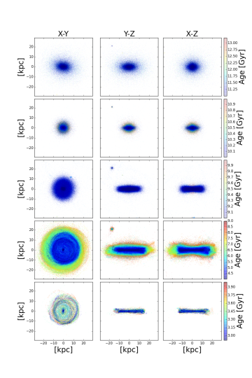
Figure 1.— Face on (first column) and edge on view (last two columns) of stars in our simulated Milky Way sized galaxy. Each row correspond to a different stellar age. From top to the bottom, 11$-$13.467 Gyr, 10$-$11 Gyr, 9$-$10 Gyr, 4$-$9 Gyr and 0$-$4 Gyr. Color code indicates stellar age.

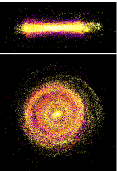
Figure 2.— Edge on (top) and face on (bottom) views of a young stellar population (0$-$7 Gyr) of model G.323 at z=0. Both Panels span 50 kpc in the x-axis. The y-axis span 22 kpc in the top panel and 50 kpc in the bottom. Color code indicates stellar age, qualitatively.

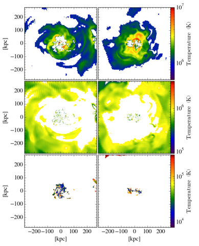
Figure 3.— Face on (left) and edge on (right) views of gas density at z=0 in model G.323, as function of its temperature. From top to the bottom, 10${}^{6}-$10⁷ K, 3$\times$10${}^{5}-$10⁶ K and 10${}^{3}-$3$\times$10⁵ K. In color we show the gas temperature.

3. GARROTXA MW-sized runs

3.1. General properties

In this work we focus mostly in three MW-sized models (G.3 series) that differ only in the aggresivity on the refinement criteria. Parameters that control the refinement aggresivity (f_DM, f_g) take the following values: (1.,1.) for the less aggressive model, (4.,8.) for the intermediate and (8., 32.) for the more aggressive. These models are the ones we have found to be in a better agreement with observed properties of the MW. The spatial resolution of all our models is high, around 109 pc. Model G.321 is the one with a lightest refinement, G.322 has intermediate conditions and G.323 is the one with hardest refinement conditions (harder means that the code uses a lower mass threshold for the refinement). All parameters we present in this section are summarized and compared with recent MW-sized models and with its observational values in Tab. LABEL:tab:1. In the table we see that there are parameters which are very sensitive to a change in the refinement setting as, for example, the SFR(z=0) that changes from 0.02 to 0.32, G.322 and G.323, respectively. Yet, most parameters do converge as can be seen in Tab. LABEL:tab:1; in particular, circular velocities profiles agree within 5% (see Appendix A for more information).
To ensure numerical convergence we also generated a low resolution model. Comparison between models can be found in the Appendix A.

3.1.1 Morphology

At z$\sim$0 our three G.3 models are massive spiral galaxies with several non-axisymmetric structures in the disk such as bars or spirals (see Fig. 1 and 2). Their assembling history is quiet after z=1.5 and the last major merger occurs at z=3. In Fig. 1 we show the face on (first column) and edge on (last two columns) views of stars of our model G.323 at z=0. For the other two models the main picture is similar but with a smaller number of stellar particles. Each row correspond to a different stellar age (see figure caption). In this figure it can be observed that young stellar component (0$-$4 Gyr) is distributed in a flat disk structure. On the other hand, older stellar populations (4$-$10 Gyr) are also distributed into a disk structure but in these cases not as flat as the younger. We argue that disk scale height and length depends on the age of the stellar population and that the former is higher and the latter is smaller when the population gets older, this issue will be addressed in Sec. 3.4.2. Another interesting property that can be easily observed in the edge on views of our models is that stellar population has an evident flare that is more evident for older populations. The face on view of the younger stellar population shows the presence of rings, spiral arms and also a young bar, in the disk. Spirals, rings and the young bar can be better observed in models G.322 and G.323 where the number of stellar particles is higher (see Fig. 2). The young bar has grown from disk particles that have ages between 0 and 8$-$9 Gyr. The old stellar population (11$-$13.476 Gyr) is distributed in a bar/ellipsoid component and it has been originated in the last major merger at z=3 (Valenzuela et al. in preparation). In Fig. 3 we show how the gas component as function of temperature (see figure caption). In this figure is easy to see that gas distribution is not isotropic. Gas is distributed in different regions of the system depending on its temperature: cold gas is present in the young stellar disk region and hot gas fills the out-of-plane region and is embedded in the DM halo. It is also interesting to see how cold/intermediate gas has a warped structure that is also marginally observed in the stellar component.

3.1.2 Stellar, gas and dark matter virial mass

Here we define the virial radius (r_vir) as the one where the sphere of radius r_vir encloses a mean density 97 times denser than the critical density ($\rho_{crit}$) of a spatially flat Universe $\rho_{crit}$=3H²(z)/(8$\pi$G). We have used value 97 as it is the value derived from the spherical top-hat collapse model for $\Lambda$CDM at z=0 for our cosmology (Bryan & Norman, 1998). This virial radius definition is borrowed from structure growth theory and then its use is not appropriated when one wants to define a physically meaningful halo edge (Cuesta et al., 2008; Zemp, 2014). To avoid this problem we also give the properties for another commonly used definition which is r₂₀₀, the radius that encloses a mean density equal to 200 times $\rho_{crit}$. Using the first definition we have obtained that the virial radius at z=0 is r${}_{vir}\sim$230 kpc in our three main models and that the mass enclosed in this radius is M_vir=7.20$-$7.61$\times$10¹¹ M_⊙. This value for the M_vir falls well inside the observational range that is M_vir=0.6$-$2.4$\times$10¹² M_⊙ by Xue et al. (2008), Kafle et al. (2012), Boylan-Kolchin et al. (2013) and Kafle et al. (2014). The total mass enclosed at r₂₀₀=175.6 kpc is M₂₀₀=6.71$-$6.90$\times$10¹¹ M_⊙. Total virial mass is distributed in dark, stellar and gaseous matter as follows: M_DM=5.86$-$6.79$\times$10¹¹ M_⊙, M_∗=6.1$-$6.2$\times$10¹⁰ M_⊙ and M_gas=1.73$-$2.70$\times$10¹⁰ M_⊙. The baryonic fraction of our G.3 models is F_b,U=0.104$-$0.121. These values are 19$-$31% smaller than the universal value for the adopted cosmology which is F_b,U=0.15. Inside r_vir, and for the model G.321, we have a total number of particles of N_total=7.52$\times$10⁶, where N_DM1sp=7.12$\times$10⁶ and N_∗=3.94$\times$10⁵ and a total number of gas cells of 2.0$\times$10⁶. For models with a more aggressive refinement the number of stellar particles and gas cells grow up to 2.34$\times$10⁶ and 6.8$\times$10⁶, respectively. All dark matter particles inside virial radius belong to less massive DM specie (1sp) and have a mass of 9.25$\times$10⁴ M_⊙. Star particles have masses between $\sim$10³ and 1.2$\times$10⁶ M_⊙. All these parameters are summarized in Tab. LABEL:tab:1.

3.1.3 Circular velocity curves

Circular velocity curves of our main simulations, computed using the $\sqrt{GM_{<r}/r}$ approach, are shown in Fig. 4 top left panel, as a solid black line. Circular velocity curves have also been computed using the real galactic potential by using Tipsy package. Results obtained using both techniques are in good agreement. Fig. 4 also shows circular velocity curves from other state of the art MW-sized simulations: Klypin et al. (2002) B1 model (blue), Mollitor et al. (2015) model (magenta), Guedes et al. (2011) ERIS simulation (green). As a comparison we show in red the analytical fit to the Sofue et al. (2009) MW rotation curve data, presented in Pichardo et al. (2003). Solid lines are the total circular velocity curves while the DM, stellar and gas components are shown as long dashed, dotted and short dashed lines, respectively. In the top right panel we show, first, G.321 velocity rotation curves of stars and gas, computed as the mean of the tangential velocity in rings centered to the galactic center (cyan solid and dashed lines), and the total circular velocity curve obtained using V_c=$\sqrt{GM_{<r}/r}$ approach. As expected, gas follows the circular velocity while stars are affected by the asymmetric drift. In this panel we also compare stellar rotation curve of our simulation (cyan solid line) with values from MW observations. We show rotation velocity curve estimations from blue horizontal-branch halo stars in the SDSS (Xue et al., 2008) (cyan and magenta dots), from Sofue et al. (2009) (red dots) and from observations of López-Corredoira (2014) (green dots). In the bottom panel we compare the recent data for the circular velocity curve obtained by Reid et al. (2014), using high mass star forming regions, with the total circular velocity curve of our G.321 model. As can be seen in the figure our G.3 models are in a a very good agreement with the most recent observational data. We also show the recent hypothetical gaseous rotation curve of the Milky Way obtained by Chemin et al. (2015) after correcting for bar non-circular motions. It is important to mention that we only show results for G.321 model because circular velocity curves of models G.322 and G.323 do not differ significantly. The peak of z=0 circular velocity of our models is reached at R${}_{peak}\sim$5.69 kpc with a value of V_c(R_peak)=237.5$-$243.8 km s^-1, the value at a standard solar radius (R_⊙=8 kpc) is V_c⊙=233.3$-$239.8 km s^-1. Also the ratio between circular velocity at 2.2 times disk scale radius (V_2.2) and circular velocity at r₂₀₀ (V₂₀₀) of our simulations (V_2.2/V${}_{200}\sim$1.9) is inside the observational range for the MW that is 1.67${}^{+0.31}_{-0.24}$ $-$ 1.11${}^{+0.22}_{-0.20}$ (Xue et al., 2008; Dutton et al., 2010).
An interesting exercise has been to compare circular velocity curves of our simulations with the one of Guedes et al. (2011) model. We have easily seen that our simulations have a bit higher velocity curves and do not present a peak in the inner regions as in Guedes et al. (2011). In simulations this internal peak is usually associated with the presence of a massive bulge in the central parts of the simulated galactic system. On the other hand, a similar peak in the V_c is shown in observational work of Sofue et al. (2009). It is in discussion whereas this peak detected in Sofue et al. (2009) observations is a signature of non-circular motions inside the bar or of a massive bulge (Duval & Athanassoula, 1983; Chemin et al., 2015). Non-circular motions need to be computed to solve such question. We plan to undertake this work in a near future following the one started by Chemin et al. (2015).
Finally, despite of the rotation and circular velocity curves we introduce here fall well inside observational ranges it is important to take into account that nowadays observational uncertainties are still high.

Table 1Parameters of GARROTXA321 (G.321), GARROTXA322 (G.322) and GARROTXA323 (G.323) simulations at z=0. r_vir is assumed to be equal to r₉₇. Mass related parameters: M_vir is total mass inside r_vir. M_∗ and M_gas are total stellar and gas mass inside r_vir. Hot, warm and cold gas mass (M_hotgas , M_warmgas, M_coldgas) are gas mass inside r_vir with temperature T $>$ 3$\times$10⁵ K, 3$\times$10⁵ K $>$ T $>$ 3$\times$10⁴ K and T $<$ 3$\times$10⁴ K, respectively. F_b,U is the baryonic fraction (M_gas+∗/M_vir), m_DM1sp is the mass of a single particle belonging to the first DM mass specie, m_∗min/max is the lowest and highest mass of stellar particles and m_SPH is the mass of SPH particles. Structural parameters: c is the DM halo concentration parameter defined as r_vir/r_s, R_d is the disk scale length, h_z,young/old is the disk scale height of young (0$-$0.5 Gyr) and old (4.0$-$11.0 Gyr) stellar populations and $\alpha_{X}$ is the hot gas density power-law exponent ($\rho_{hotgas}$(r) $\propto$ r${}^{\alpha_{X}}$). Kinematical parameters: V_c⊙ is the circular velocity at solar position (R_⊙ = 8 kpc), R_peak is the radius in where circular velocity curve reaches its highest value (V_c(R_peak)). Initial condition parameters: n_SF, T_SF and $\epsilon_{SF}$ are the star formation density and temperature thresholds and the star formation efficiency. Box is the simulated box size in Mpc h^-1, z_ini is the initial redshift and $\Omega_{0}$, $\Omega_{\Lambda}$, $\Omega_{b}$, H₀ and $\sigma_{8}$ define the assumed cosmological model. Comparison with other state of the art simulations is also shown (ERIS simulation (Guedes et al., 2011) and model B in Mollitor et al. (2015)). Observed values for the MW have been obtained from Ferrière (2001); Flynn et al. (2006); Du et al. (2006); Hammer et al. (2007); Xue et al. (2008); Jurić et al. (2008); Dutton et al. (2010) and Kafle et al. (2014), see text for more details on references.

	rvir	Mvir	M∗	Mgas	Mhotgas	Mwarmgas	Mcoldgas
	[kpc]	[M⊙]	[M⊙]	[M⊙]	[M⊙]	[M⊙]	[M⊙]
G.321	230.1	7.33$\times$1011	6.1$\times$1010	2.70$\times$1010	1.22$\times$1010	5.66$\times$109	9.34$\times$109
G.322	230.1	7.20$\times$1011	6.1$\times$1010	1.73$\times$1010	0.98$\times$1010	5.98$\times$109	1.52$\times$109
G.323	230.1	7.61$\times$1011	6.2$\times$1010	1.96$\times$1010	1.32$\times$1010	4.54$\times$109	1.86$\times$109
ERIS	239.0	7.90$\times$1011	3.9$\times$1010	5.69$\times$1010	3.60$\times$1010	14.20$\times$109	6.70$\times$109
MollitorB	234.0	7.10$\times$1011	5.6$\times$1010	7.96$\times$1010	$-$	$-$	$-$
MW obs.	$-$	1.0$\pm$0.30$\times$1012	4.9-5.5$\times$1010	$-$	$-$	$-$	7.3$-$9.5$\times$109
	r200	M200	Fb,U	mDM1sp	m∗min	m∗max	mSPH
	[kpc]	[M⊙]		[M⊙]	[M⊙]	[M⊙]	[M⊙]
G.321	175.6	6.84$\times$1011	0.120	0.93$\times$105	0.24$\times$104	120.0$\times$104	$-$
G.322	175.6	6.71$\times$1011	0.109	0.93$\times$105	0.12$\times$104	120.0$\times$104	$-$
G.323	175.6	6.90$\times$1011	0.107	0.93$\times$105	0.12$\times$104	120.0$\times$104	$-$
ERIS	175.0	6.60$\times$1011	0.120	0.98$\times$105	0.63$\times$104	0.63$\times$104	2.0$\times$104
MollitorB	176.5	6.28$\times$1011	0.191	2.30$\times$105	4.50$\times$104	4.50$\times$104	$-$
MW obs.	$-$	$-$	$-$	$-$	$-$	$-$	$-$
	Npart	NDM1sp	N∗	Ngas	Resolution	CPU time	CODE
	[106]	[106]	[106]	[106]	[pc]	[104 h]
G.321	7.52	7.12	0.39	2.0	109(1cell)	2.5	ART + hydro
G.322	7.95	7.08	0.86	5.0	109(1cell)	4.3	ART + hydro
G.323	9.44	7.10	2.34	6.80	109(1cell)	9.2	ART + hydro
ERIS	15.60 (+SPH)	7.00	8.60	3.0	120($\epsilon$)	160.0	GASOLINE (SPH)
MollitorB	6.06	3.91	2.15	2.50	150(1cell)	$-$	RAMSES (hydro)
MW obs.	$-$	$-$	$\sim$100000.0	$-$	$-$	$-$	$-$
	c=rvir/rs	Rd	hz,young	hz,old	Mhotgas/Mvir	$\alpha_{X}$	SFR (z=0)
		[kpc]	[pc]	[pc]			[M⊙ yr-1]
G.321	28.5	2.56 (4.89/2.21)	277 (exp)	1356	0.016	-0.62	0.27
G.322	26.8	3.20 (5.26/2.26)	295 (exp)	960	0.013	-0.83	0.02
G.323	26.9	3.03 (3.19/3.31)	393 (exp)	1048	0.017	-0.67	0.32
ERIS	22.0	2.50	490 (sech2)	$-$	0.017	-1.13	1.10
MollitorB	56.5	3.39	$-$	$-$	0.046	-4.54	4.75
MW obs.	21.1${}^{+14.8}_{-8.3}$	2.0$-$4.5	300$\pm$60	600$-$1100$\pm$60	$-$	$-$	0.68-1.45
	Vc⊙(R=8 kpc)	Rpeak	Vc(Rpeak)	V2.2/V200	nSF	TSF	$\epsilon_{SF}$
	[km s-1]	[kpc]	[km s-1]		[cm-3]	[103 K]
G.321	239.8	5.69	243.8	1.90	1.0	9	0.65
G.322	233.6	5.69	237.5	1.85	1.0	9	0.65
G.323	233.3	5.69	237.8	1.93	1.0	9	0.65
ERIS	206.0	1.34	238.0	1.66	5.0	30	0.10
MollitorB	233.0	9.63	233.0	$-$	2.7	3	0.01
MW obs.	221$\pm$18	$-$	$-$	1.11${}^{+0.22}_{-0.20}$	$-$	$-$	$-$
	Box	zini	$\Omega_{0}$	$\Omega_{\Lambda}$	$\Omega_{b}$	H0	$\sigma_{8}$
	[Mpc h-1]					[km s-1 Mpc-1]
G.321	20	60	0.30	0.70	0.045	70	0.80
G.322	20	60	0.30	0.70	0.045	70	0.80
G.323	20	60	0.30	0.70	0.045	70	0.80
ERIS	90	90	0.24	0.76	0.042	73	0.76
MollitorB	20	50	0.276	0.724	0.045	70.3	$-$
MW obs.	$-$	$-$	$-$	$-$	$-$	$-$	$-$

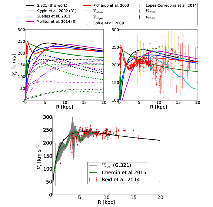
Figure 4.— Top-left: Circular velocity curve of our simulated Milky Way sized galaxy model G.321 (black), Guedes et al. (2011) (green), model B1 in Klypin et al. (2002) (blue), Mollitor et al. (2015) (magenta) and analytical model in Pichardo et al. (2003) (red). The figure shows the contribution to the circular velocity V_c=$\sqrt{GM_{<r}/r}$ of dark matter (short dashed curve), stars (long dashed), gas (dot-dashed) and total (solid curve) mass components. Top-right: Total circular velocity curves of the same models shown at left, observational data points and gas and stars rotation curves of our model G.321 (cyan dashed and solid lines, respectively). Data points come from two realizations of the rotation curve of the Milky Way from observations of blue horizontal-branch halo stars in the SDSS (Xue et al., 2008), in cyan and magenta dots, from López-Corredoira (2014), in green, and from Sofue et al. (2009), in red. Bottom: Observational circular velocity curve obtained using massive young star forming regions of the MW (Reid et al., 2014). The total V_c of our model G.321 at z=0 is shown as a black solid line. In green we show the hypothetical gaseous rotation curve of the Milky Way obtained by Chemin et al. (2015) after correcting the non-circular motions in the velocity profile of the Milky Way inferred with the tangent-point method by Kalberla et al. (2005). In grey we show Chemin et al. (2015) curve 1$\sigma$ range.

3.2. Dark matter component

As we have mentioned in the last section all dark matter particles inside virial radius are particles of the first DM specie, the less massive one. In Fig. 5 we show the dark matter density profile as a function of radius (red circles) and the best fit of NFW profile for the model G.321 (upper yellow solid line). We avoid the central region (R $<$ 5 kpc) in the fit of the NFW profile to avoid perturbations derived from the presence of baryons (adiabatic contraction). The best NFW fit gives a large value for the halo concentration that is c=r_vir/r_s=28.5, 26.8 and 26.9 for G.321, G.322 and G.323, respectively. These values fall inside the observational range presented in Kafle et al. (2014) that is 21.1${}^{+14.8}_{-8.3}$. No core is observed in the central region of our G.3 models. The halo spin parameter as defined in Bullock et al. (2001) is $\lambda$’=0.019, 0.017 and 0.022. These $\lambda$’ values also fall near the range obtained by Bullock et al. (2001) after analyzing more than 500 simulated halos (see figure 1 and 2 in Bullock et al. (2001)).

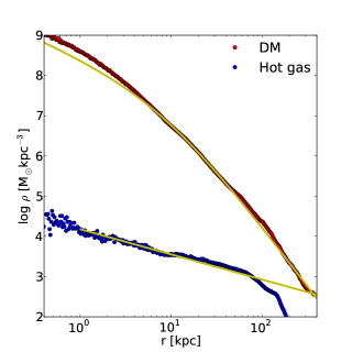
Figure 5.— Average dark matter (red dots) and hot gas (T $>$ 3$\times$10⁵ K, blue dots) density profiles at z=0. The upper solid yellow line show the best NFW profile fit to the dark matter mass distribution, in the range from 5 kpc, outside bar-bulge region, to r_vir. The lower solid yellow line show the best fit power-law profile to the hot gas mass distribution between 5 and 20 kpc. The DM best fit NFW profile is characterized by a large halo concentration parameter c=28.5 as the dark matter halo contracts in response to the condensation of baryons in its center (adiabatic contraction). In the inner region it can be clearly observed that no DM core is present. The hot gas best fit power-law profile gives a slope of $\alpha_{X}$=-0.62.

3.3. Gas component

In our models G.321, G.322 and G.323 the total gas mass inside the virial radius is M_gas=2.7, 1.73 and 1.96 $\times$10¹⁰ M_⊙. In G.321, 9.34$\times$10⁹ M_⊙ of gas mass is in the cold gas phase (T $<$ 3$\times$10⁴ K). In G.322 and G.323 cold gas mass is 1.52 and 1.86$\times$10⁹ M_⊙. The cold gas mass in G.321 is comparable to the total mass of the molecular, atomic and warm ionized medium inferred for the MW that is $\sim$7.3$-$9.5$\times$10⁹ M_⊙ (Ferrière, 2001). For the rest of models presented here the amount of cold gas is smaller than the observed value. This z=0 cold gas mass reduction is consequence of an increase on the star formation at early ages, that in its turn is provoked by the higher aggresivity in the refinement criteria. This increase on the early star formation is the only significant effect we have observed when changing the refinement criteria and it is consequence of resolving a larger number of small dense regions in where the SF criteria is accomplished.
At z=0, the SF criteria is satisfied only in the inner disk regions (R $<$ 7 kpc). This spatially limited star formation accords with the young stellar distribution shown in Fig. 1 and also with the decrease of the Star Formation Rate (SFR) at z=0 that can be seen in Fig. 10.

The hot gas mass (T $>$ 3$\times$10⁵ K) is around 1.22, 0.98 and 1.32$\times$10¹⁰ M_⊙ for models G.321, G.322 and G.323, respectively. The definition of hot gas we use in this work is observationally motivated: total hot gas mass has to be inferred from ionized oxygen observations (Gupta et al., 2012) and this is only possible when gas has opacity in the X-ray region (T $>$ 3$\times$10⁵ K). In Fig. 3 we show the gas distribution as function of temperature in model G.323. Each panel show the distribution of gas at different temperatures (see figure caption). As can be seen in this figure cold gas is placed in disk region while warm-hot is embedded within the dark matter halo. Contrary to the standard assumption, hot gas do not follow the dark matter radial distribution. This can be seen in Fig. 5 where we show the dark matter density distribution (red) and the hot gas density distribution (blue). The hot gas density distribution inside r = 100 kpc can be fitted by a power law ($\rho_{hotgas}$(r) $\propto$ r${}^{\alpha_{X}}$). After fitting data from models G.321, G.322 and G.323 we have obtained that hot gas density distribution scale factors ($\alpha_{X}$) of these models are -0.62, -0.83 and -0.67, respectively. These results are slightly higher than values used to fit analytical models of hot gas in dark matter halos (-0.9 in Anderson & Bregman, 2010) and the ones obtained in other similar models like ERIS (-1.1 in Guedes et al., 2011). The hot gas density distribution power law fit for model G.321 is shown in Fig. 5 (bottom yellow straight line).

In Sec. 4 we present our first results on the study of hot gas distribution and a comparison with observational values.

3.4. Stellar component

The total stellar mass in the virial radius of our G.3 models is M_∗=6.1$-$6.2$\times$10¹⁰ M_⊙, that is comparable with values estimated for the Milky Way (4.5$-$ 7.2$\times$10¹⁰ M_⊙ in Flynn et al. (2006) and Licquia & Newman (2015)). However, if we observe the relation between stellar mass and total mass (see Fig. 6) derived from our models (blue dots) and also from observations of the MW (shadowed region) we see that most of them fall quite above the M_∗/M_vir predicted by cosmological theories. The same result is observed when using data from other recent MW-sized simulations like ERIS simulation (Guedes et al., 2011) or the ones of Mollitor et al. (2015). In this work we have not studied this mismatch deeply, we leave it for the future.

3.4.1 Stellar disk and stellar spheroid

Simulated galactic systems in our main models (G.3 series) have both stellar disks and stellar spheroidal components (halo and/or bulge). To study properties of stellar galactic disks we need to know which stars belong to it. To undertake the selection process we have used an extension of the kinematic decomposition proposed by Scannapieco et al. (2009). In Scannapieco et al. (2009) the authors used the ratio between the real stellar particle angular momentum perpendicular to the disk plane ($j_{z}$) and the one obtained assuming stellar particles follow a circular orbit (computed from the circular velocity curve, $j_{c}$). The circular velocity curve has been computed using both, GM/r approach and the real galactic potential; we have found that results do not depend on the v_c computation technique. Using $j_{z}/j_{c}$ ratio it is possible to distinguish particles that are rotationally supported ($j_{z}$=$j_{c}$ for disk stars) from ones that are not ($j_{z}$ $<$ $j_{c}$ for spheroid stars). Here we have decided to make additional cuts to improve this technique. We have done complementary cuts in metallicity, in the vertical coordinate $\left|z\right|$, in the angle between the rotation axis of each particle and the vector perpendicular to the plane ($cos(\alpha)$) and in the distance to the galactic center (R). To avoid kinematic biases we have made cuts that do not involve kinematics first. We have started the selection process by making the metallicity cut; next, we have made a cut in the vertical coordinate, and later in radius, in $cos(\alpha)$; finally we have used $j_{z}$/$j_{c}$ condition. Some of these restrictions we have imposed require from a previous knowledge of the disk plane position. To find this position we have used an iterative geometrical approach (pages 9 to 11 in Atanasijevic, 1971). In this approach we end up with the plane that minimizes the cumulative distance of all particles to it. In the first iteration of this process we only use stars that are inside a 20 kpc sphere centered within the center of mass of the lightest DM mass specie particles. After this first iteration we only use stars that fall nearby the newly defined plane (i.e. $\left|z_{new}\right|$ $<$ 5 kpc). We have checked that after few iterations we get a plane that coincides with the disk plane defined by young stars and cold gas (see bottom panels of Fig. 1, Fig. 2 and Fig. 3).
After analyzing the stellar distribution of our G.3 models in both, Cartesian and phase spaces, we have found conditions that better distinguish disk from spheroid particles. In our main models these conditions are: $j_{z}$/$j_{c}$ $>$ 0.55, $\left|z\right|$ $<$ 3.5 kpc, log(ZIa/ZIa_⊙) $>$ -0.5, where ZIa_⊙ = 0.00178 and it is the iron solar abundance according to Asplund et al. (2009), cos$(\alpha)$ $>$ 0.7 and R $<$ 25 kpc. All particles inside r${vir}$ that do not accomplish one or more of these restrictions are considered spheroid particles (halo and/or bulge particles). To account for thick disk particles we relax the log(ZIa/ZIa_⊙) and $j_{z}$/$j_{c}$ conditions; that is, stellar particles will also belong to the disk component if they fulfill all previous conditions except that they have log(ZIa/ZIa_⊙) $<$ -0.5 and $j_{z}$/$j_{c}$ deviates by less than 0.75 from $j_{z}$/$j_{c}$ peak. The result of this selection can be seen in Fig.7 where we show the stellar mass fraction as a function of $j_{z}$/$j_{c}$ for model G.321, the result is similar for the other models. In this figure we show how well we trace the two main stellar components of the model: one centered at $j_{z}$/$j_{c}$=1, i.e. rotationally supported, and another at $j_{z}$/$j_{c}$=0.

The mass of the rotationally supported component (stellar disk) is around M_d = 1.82, 2.17, 2.21$\times$10¹⁰M _⊙ and that of the spheroidal one (bulge + halo) is M_sp = 4.29, 3.93, 3.79$\times$10¹⁰ M_⊙ for models G.321, G.322 and G.323, respectively. Comparing these results with observations we find that the mass of the spheroidal component in our models (bulge + halo stars) is higher than the upper limit obtained by Flynn et al. (2006) which is M_b $\leq$ 1.3$\times$10¹⁰ M_⊙ or than the most recent observations presented by Valenti et al. (2016) (M_b=2.0$\pm$0.3$\times$10¹⁰ M_⊙). The spheroids of our galactic systems are $\sim 2$ times heavier than the one of the MW. On the other hand, disks in our G.3 models are less massive than the one estimated for the MW by Bovy & Rix (2013) ($\sim$4.6$\times$10¹⁰ M_⊙). As a consequence, the kinematic disk-to-total ratio (D/T) decomposition, f_disk, computed as M_∗disk/M_∗ (Scannapieco et al., 2010, 2015) where M_∗disk is the mass of stellar particles with j_z/j_c $>$ 0.5, results in a value ($\sim$0.42) that is significantly lower than the one obtained in MW observations ($\sim$0.75 in Scannapieco et al., 2011). However, as pointed out by Scannapieco et al. (2010, 2015) the use of a kinematical decomposition results in a lower D/T than those obtained using a photometric decomposition, as the one determined in MW observations. For instance, in Scannapieco et al. (2010) the authors obtained a set of MW-sized galaxies with a kinematical f_disk $\sim$ 0.2 and they demonstrated that f _disk becomes 0.4$-$0.7 when using a photometric decomposition.

Is the presence of this massive spheroidal component due to a large stellar concentration in the central region of our simulated galaxies, a common result in earlier hydrodynamical zoom-in simulations? As can be seen in the rotation curves shown in Fig. 4 this is not the case (the curves do not present a central peak). We have analyzed this spheroidal component and we have detected that it is mainly a triaxial structure that was formed in the major merger occurred at z = 3 (see Sec. 3.1.1). This triaxial structure has a low density in the disk region and thus it is not a classical massive bulge.

3.4.2 Disk properties

With the stellar disk/spheroid selection process we have found that disk component has 2.0, 6.0 and 18.7$\times$10⁵ particles in each one of our main G.3 models. We have also computed the mean volume and surface density of the disk, as function of radius. We have found that a single or a double exponential power law can be fitted to the data depending on the age of the selected population. In Fig. 8 we show the total disk surface density (black) as function of radius of the model G.321 at z=0. We have fitted two exponential power laws (red and blue) to the surface density curve. Results from these fits are that scale length in the inner regions (2$-$6 kpc) is R_d=4.89 kpc and in the outer ones (6$-$12 kpc) R_d=2.21 kpc. If we fit a single exponential to the whole radial range from 2 to 12 kpc we obtain that R_d=2.56 kpc, result that is in agreement with values obtained for the MW (e.g. 2.3$\pm$0.6 kpc in Hammer et al. (2007) or 2.15$\pm$0.14 kpc in Bovy & Rix (2013) using G-type dwarfs from SEGUE). It is important to note that, as can be seen in Fig. 8, a small concentration of stars is present in the central regions (R $<$ 2 kpc). This concentration is caused by the presence of a young bar.
In Fig. 9 we show the volume density as function of the distance to the plane (z) of three disk stellar populations split by age. We have selected a young (0$-$0.5 Gyr), intermediate (0.5$-$4.0 Gyr) and old (4.0$-$11.0 Gyr) populations. The density have been computed using vertical bins of $\Delta$z=0.2 kpc and only stellar particles that are in between R=2 and R=9 kpc. We have found that the scale height (h_z) of each population, when fitting a decreasing exponential to the vertical density distribution in the range 0.1 kpc $<$ $\left|z\right|$ $<$ 2.0 kpc, is h_z=277 pc for the young, h_z=959 pc for the intermediate and h_z=1356 pc for the old populations. These values have been obtained from G.321 model, results from models G.322 and G.323 can be found in Tab. LABEL:tab:1. These scale height values are compatible with ones expected for the MW: observations show that the vertical distribution of stars in the MW can be fitted by two exponential with a scale heights of h_z=300$\pm$60 pc (Jurić et al., 2008) and h_z=600$-$1100$\pm$60 pc (Du et al., 2006). Our values also follow the relation proposed by Yoachim & Dalcanton (2006) that argue that disk scale height in edge on galaxies increases in disks following z${}_{0}\approx$2h_z=610(V_c/100) km s^-1.

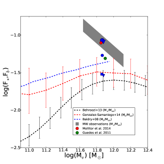
Figure 6.— Comparison between stellar/baryonic fraction (F_∗,b = M_∗,b/M_vir) theoretical predictions and the ones obtained from observations and simulations. Blue items show M_∗/M_vir values in our models G.321 (circles), G.322 (triangles) and G.323 (squares), using total stellar mass (large items) and only disk stellar mass (small items), see Sec. 3.4.1 for information about stellar disk selection process. Observed range for the M_∗/M_vir in the Milky Way Galaxy (Flynn et al., 2006; Xue et al., 2008; Licquia & Newman, 2015; Gibbons et al., 2014) is shown as a grey shadowed region. Red dot show the M_∗/M_vir value obtained in model B presented by Mollitor et al. (2015). Green dot shows M_∗/M_vir of the ERIS simulation (Guedes et al., 2011). Behroozi et al. (2013) observational M_∗/M_vir curve inferred from observations at z=0.1, with no distinction between blue or red galaxies, and its errors, is shown as dashed black line. As a red dashed line, results obtained for the M_b/M_vir relation in González-Samaniego et al. (2014) when using a semi-empirical model. The blue dashed line corresponds to the M_b/M_vir relation calculated by Baldry et al. (2008). As can be seen it becomes a challenge for $\Lambda$CDM to fit its theoretical predictions with observations.

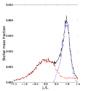
Figure 7.— Stellar mass fraction as function of the orbital circularity parameter j_z/j_c, describing the degree of rotational support of a given stellar particle (black: all particles; red: spheroid; blue: disk). The stars in a centrifugally supported thin disk manifests itself in a sharply peaked distribution about unity. We have plotted only stellar particles inside disk region ($\left|z\right|$ $<$ 0.5 kpc and r $<$ 15 kpc) of model G.321 at redshift 0.

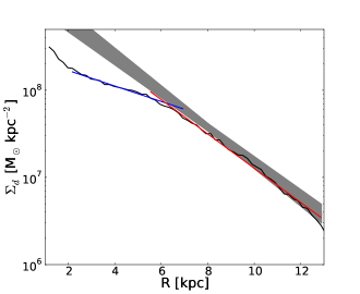
Figure 8.— Stellar disk surface density profile as function of cylindrical radius R (black solid line). The solid blue and red lines show the best-fit exponential profiles to the inner and outer disk components, respectively. The inner component (2$-$6 kpc) has an R_d=4.89 kpc and the outer (6$-$12 kpc) an R_d = 2.21 kpc. If we fit the whole disk density profile from 2 to 12 kpc we obtain an R_d = 2.56 kpc. All results have been obtained analyzing model G.321 at redshift 0. As a gray shadowed region we show MW surface density profile obtained by Bovy & Rix (2013).

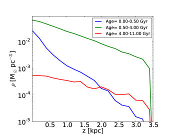
Figure 9.— Vertical density profile of young (blue), intermediate (green) and old (red) disk stars in the model G.321 at redshift 0.

3.4.3 Star formation history (SFH)

In our simulations stars are being formed with a SFR_z=0=0.27 M_⊙ yr^-1, 0.18 M_⊙ yr^-1 and 0.41 M_⊙ yr^-1, for models G.321, G.322 and G.323, respectively. These values are smaller than ones inferred by Robitaille & Whitney (2010) using Spitzer data, for the MW (SFR=0.68$-$1.45 M_⊙ yr^-1) or the one from Licquia & Newman (2015) that is 1.65$\pm$0.19 M_⊙ yr^-1. In Fig. 10, top panel, we show the SFR as function of the redshift for the total (black), spheroidal (red) and disk (blue) components. We have computed the SFH of each stellar component using the formation time of their corresponding stellar particles (saved by the code) inside r_vir at z=0. We have followed the strategy described in Sec. 3.4.1 to distinguish between disk and spheroid stellar particles. We also show, as a shadowed region, the predicted SFH for MW like halos derived from semi-analytical models that combine stellar mass functions with merger histories of halos (Behroozi et al., 2013). The peak in the SFH of our G.3 models occurs at slightly early ages than the one predicted for a MW-sized galaxy. In the bottom panel we plot the total stellar mass as function of redshift. Some important results that can be appreciated from this figure are, first, that the spheroidal component is being build at high redshifts while disk starts its formation at around z=2.5 ($\sim$11 Gyr from the present time), just after the last major merger that was at z=3. Second, it is also important to note that the star formation of spheroidal component decrease quickly after z$\sim$2.4 and become negligible at around z=0.5. The disk SFR also decreases fast in the last time instants except for some short periods of star formation that are a consequence of the accretion of small gaseous satellites. This reduction in the star formation when reaching z=0 is a consequence of the reduction of cold gas available for star formation. Several processes can lead to a reduction of the cold gas mass fraction. First, cold gas can be drastically consumed at higher redshifts due to a non-realistic implementation of physical parameters that controls star formation (Liang et al., 2016). When such problem exists a large amount of old stars are present at z=0 in the inner disk region. In our G.3 models, as can be seen in Fig. 7, an old spheroid is present in the disk region, however this old stellar population is not big enough to account for the total reduction of the observed cold gas component. Second, if stellar and SNe feedback is too efficient, an important amount of cold gas can be heated up and then to become unavailable for star formation. In this second scenario what we would expect is that the fraction of hot gas increase with time, a behavior that is not observed in our G.3 models. Finally a decrease in the cold gas inflow due to inhomogeneities in the circumgalactic medium (CGM) can also be a cause of the reduction of the SFR. In this last hypothesis we would observe only a small amount of cold gas present around our system, or falling from filaments, in the last Gyr. We argue that in our models the reduction of the amount of cold gas is a consequence of a combined effect of the first and the last hypothesis as we observe that an old spheroid is present and also that there is not a large amount of cold gas falling from filaments at z=0, however we leave the deeper study of such processes for the future.

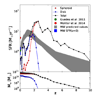
Figure 10.— Star formation history (SFH), top, and total mass history, bottom, of all star particles identified within virial radius at z=0 in model G.321. Black, blue and red filled dots show the total, disk and spheroid star formation rates (top panel) and stellar mass (bottom panel), respectively, as a function of redshift. Grey shadowed region indicates the predicted SFH for a MW-like halo with M₉₇=10¹² M_⊙ (Behroozi et al., 2013). Green and red big dots show total SFR at z=0 of models presented by Guedes et al. (2011); Mollitor et al. (2015) (B), respectively. The blue filled region shows the z=0 MW SFR range derived from observations by Robitaille & Whitney (2010).

In ART, the metallicity $Z$ is divided according to which kind of SNe produce the metals: $ZII$ or $ZIa$, if they are produced by SNII or SNIa, respectively. The metallicity $Z$ is then $Z=ZIa+ZII$. Alpha elements, as oxygen, are mostly produced by SNII while iron is mostly produced by SNIa, we thus can assume that the abundance of the former are proportional to ZII while the iron abundance is proportional to ZIa.

3.5. Are our G.3 models MW-like systems?

Although it is not the aim of this paper to obtain a realistic model of the MW galaxy, nevertheless the models we present here (i.e. G.321, G.322 and G.323) can be considered at least MW-sized as they reproduce several of the MW observed properties. On the other hand, it is also evident that some parameters of these models fall far from observations of the MW. Below, we give an overview of the parameters that match MW observations and of those ones that do not.

3.5.1 MW-like properties

Our study is focused on a galactic system, the G.3 series, that forms spiral arms and a galactic bar. Its assembly history is quiet after z=1.5 and there are no major mergers after z=3, something that is also expected for our Galaxy (Forero-Romero et al., 2011). Its total mass is inside the observational range proposed for the MW by Xue et al. (2008); Boylan-Kolchin et al. (2009); Kafle et al. (2012, 2014) that is 1.0 $\pm$ 0.4 $\times$ 10¹² M_⊙. The stellar mass inside virial radius (6.1 $-$ 6.2 $\times$ 10¹⁰ M_⊙) falls also inside the observational range for the MW that is 4.5 $-$ 7.2 $\times$ 10¹⁰ M_⊙ (Flynn et al., 2006; Licquia & Newman, 2015). Finally, the cold gas mass inside virial radius in model G.321 (9.34 $\times$ 10⁹ M_⊙) also match the observed values (7.3 $-$ 9.5 $\times$ 10⁹ M_⊙ in Ferrière (2001)). Several structure parameters of our G.3 models are also within the MW observations. This is the case for the dark matter halo concentration parameter (c) that in our models takes values from 26.8 to 28.5 while observations predict it should be 21.1${}^{+14.8}_{-8.3}$ (Kafle et al., 2014). Hot gas power-law profile index ($\alpha_{X}$), defined in Sec. 3.3, and that in our G.3 models is in between -0.62 and -0.83, is also close to value proposed by Anderson & Bregman (2010) which is -0.9. Disk scale lengths and heights of our galactic systems (G.3 series) also coincide or are close to observed values. The former in our models is 2.56$-$3.2 kpc and observed values are 2.3$\pm$0.6 kpc in Hammer et al. (2007) and 2.15$\pm$0.14 in Bovy & Rix (2013). Observed disk scale height of young and old stars is 300 $\pm$ 60 pc in Jurić et al. (2008) and 600$-$1100 pc in Du et al. (2006), respectively, and in our models we have obtained for young and old populations, 277$-$393 pc and 960$-$1356 pc, depending on the model. Finally, also several kinematical parameters agree with the MW observations; the rotation curve of our simulated galaxies, for instance, roughly match observations (see Fig. 4). Some examples of such agreement are the ratio V_2.2/V₂₀₀ that is 1.9 in our models and 1.67${}^{+0.31}_{-0.24}$ in Xue et al. (2008), and the v_c(R_⊙) that is 233.3$-$239.8 km s^-1 in this work and 221$\pm$18 in Koposov et al. (2010) or 236$\pm$11 in Bovy et al. (2009).

3.5.2 Parameters that do not match observations

Among the parameters that do not agree with the observed values of the MW is the SFR and the bulge to disk ratio. The cold gas fraction in the G.323 and G.323 models also do not match observations, they account for only 1.52 and 1.86 $\times$ 10⁹ M_⊙ while observed values are 7.3 $-$ 9.5 $\times$ 10⁹ M_⊙ Ferrière (2001). On the other hand, the SFR in our models ranges from 0.18 to 0.41 M_⊙ yr^-1 values below the observational range 0.68 $-$ 1.45 M_⊙ yr^-1 from Robitaille & Whitney (2010). Finally, we have presented in Sec. 3.4.1 the stellar spheroid-disk decomposition and shown that a massive spheroid exists in our models. Such massive structure has not been observed in the MW. The total mass of the spheroid (bulge+halo) and the stellar disk in our G.3 models are 3.79$-$4.29 $\times$10¹⁰ M_⊙ and 1.82$-$2.21 $\times$10¹⁰ M_⊙, respectively. Moreover, observations show that the bulge and the disk mass of our Galaxy are $\leq$2.3$\times$10¹⁰ M_⊙ (Flynn et al., 2006; Valenti et al., 2016) and $\sim$4.6$\times$10¹⁰ M_⊙ (Bovy & Rix, 2013), respectively; that is, the spheroid of our models is at least two times more massive than the bulge of the MW.

4. Missing baryons problem and the X-ray luminous hot gas

4.1. The missing baryons problem

It was long been known that the cosmological baryon fraction inferred from Big Bang nucleosynthesis is much higher than the one obtained by counting baryons at redshift z=0 (e.g. Fukugita et al., 1998). However, it was recently, with WMAP and Planck high precision data of the cosmic microwave background (Dunkley et al., 2009; Planck Collaboration et al., 2014), that the cosmic baryonic fraction was well constrained and thus the lack of baryonic mass in galaxies became evident. This data revealed that the cosmic ratio between baryonic and total matter ($\Omega_{b}/\Omega_{M}$) is 3$-$10 times larger than the one observed in galaxies. For instance, Hoekstra et al. (2005) found a baryonic fraction for isolated spiral galaxies of 0.056 and for elliptical of 0.023 while Dunkley et al. (2009) presented a cosmic baryonic fraction from WMAP 5-year data of about 0.171$\pm$0.009.
Studies like Cappi et al. (2013); Georgakakis et al. (2013) tried to solve this missing baryon problem proposing that galactic winds, SNe feedback or strong AGN winds ejected baryons to the circumgalactic medium (CGM). Others proposed that most of the gas never collapsed into the dark matter halos as it was previously heated by SNe of Population III (e.g. Mo & Mao, 2004), this is known as the preheating scenario. In this last scenario missing baryons are still in the extragalactic warm-hot intergalactic medium (WHIM), following filaments. Thus, it has become clear that studying the CGM is necessary not only for finding the missing baryons, but also to understand its properties in the context of galaxy formation and evolution models. To further constrain galaxy evolution and find out which one of the proposed theories solves the missing baryon problem it is needed to measure the amount of warm-hot gas phase present in the CGM and also its metallicity. Results of such measures give information about the heating mechanism: hot gas with low metallicities is indicative of a Pop III SNe preheating while a more metallic gas suggest that it has been enriched in the disk via SNe and stellar winds.
Supporting the first hypothesis, the idea of very strong feedback driving galactic-scale winds, causing metal-enriched hot gas to be expelled out of the star-forming disk possibly to distances comparable to or beyond the virial radius was generally accepted. This process also lies in the heart of obtaining realistic simulations of disk galaxies (Guedes et al., 2011; Marinacci et al., 2014). By this mechanism gas is temporally placed far from star forming regions delaying the star formation and preventing the formation of an old bulge in the center of the system.
From the analysis of OVII and OVIII X-Ray absorption lines observed towards the line of sight of extragalactic sources, several authors performed estimations of the hot gas mass in the MW halo, suggesting that an important part of the missing baryons is located in this hot gas phase (Gupta et al., 2012, 2014). They concluded that the warm-hot phase of the CGM is extended over a large region around the MW, with a radius a mass around 100 kpc and 10¹⁰ M_⊙. However, these estimations are limited to a few directions towards extragalactic sources (bright QSOs) and as a consequence issues like the homogeneity or isotropy of the hot gas distribution possibly affecting the mass estimation are hard to be addressed by them. Other studies like Feldmann et al. (2013) also suggest that the presence of this hot gas phase can explain part of the isotropic gamma-ray background observed in Fermi Gamma-ray Space Telescope.

4.2. Hot gas component in G.321

4.2.1 Spatial distribution

The amount of hot gas in our G.3 models is in between M_hot = 0.98$-$1.32$\times$10¹⁰ M_⊙. This hot gas that has a temperature above 3.0$\times$10⁵ K (has opacity in the X-rays) is embedded in the dark matter halo but mostly outside the stellar disk. Aiming to perform a fair comparison with observations we estimated the hot gas Hydrogen equivalent column density and emission measure (EM) as:

$$N_{H}=\int_{los}n_{H}dl$$ (2)

$$EM=\int_{los}n_{e}^{2}dl$$ (3)

where n_H is the hydrogen particles density, dl is an element of the path in the line of sight and $n_{e}$ is the electron density.

In Fig.13 we show a full sky view of hot gas column density distribution in our model G.321. This figure has been obtained computing the hot gas column density from a position that is at 8 kpc from the galactic center, inside the simulated galactic disk, resembling the Sun position, and assuming arbitrary azimuthal angles. We have obtained column density values that fall near the observational ranges, if a solar metallicity is assumed (see Tab. 3 and Gupta et al., 2012). However, when assuming lower metallicities, observations are consistent with values that are above the ones measured in our simulations. This change can give us information about the absorption of the local WIMP. We also conclude that the distribution of hot gas inferred from all estimations is far from homogeneous. In order to quantify the hot gas anisotropy we followed two strategies. First we computed the amplitude of the first spherical harmonics (Y${}_{l}^{m}$ from l,m=0 to 5 ) and later we also computed the filling factor as defined by Berkhuijsen (1998). Our results show that the dominant spherical harmonic is Y${}_{1}^{0}$, that is an indicator of the dipolar component, with a small contribution of several high order components. The asymmetry of the hot gas distribution with respect to the disk plane suggest some degree of interaction with the extragalactic medium. The computation of the mean filling factor from line of sights distributed all along the sky gives as a value of f${}_{v}\sim$0.33$\pm$0.15. This value for the filling factor also suggests that hot gas is concentrated in a few regions of the sky. It is also important to mention that in our G.3 models (see Fig. 3 and 13) we do not detect a hot gas thick disk component. This is important as it is under discussion what is the contribution of the hot gas thick disk to the observed X-ray emission/absorption (Savage et al., 2003). Additionally to the spatial distribution we study the metallicity and velocity components of hot gas cells. Metallicity and velocity fields provide us information about how the hot gas component interacts with the extragalactic medium. In Fig. 14 we show the metallicity distribution of the hot gas as seen from the Galactic center. It is evident that gas metallicity distribution does not depend on the azimuthal angle ($\theta$) (Fig. 14, top panel) while it is clear the dependency on the vertical latitud ($\phi$) (Fig. 14, bottom panel). It is also noticeable a low metallicity component located at the northern hemisphere that is absent at the southern, where metallicity is in average much higher. It is important to note that in Fig. 14, bottom panel, we can distinguish a clear break in the hot gas distribution at low latitudes. This hole coincides with the position of the stellar/cold gas disk.
In order to shed some light on the bimodal origin in the metals distribution, we have analyzed a set of three color maps showing the projected metallicity and velocities along each one of the principal planes (see Fig. 15 and Fig. 16). Fig. 15 (X-Y plane, i.e. disk plane) shows that in general hot gas in the disk plane rotates following the disk rotation direction. Fig. 16 (X-Z plane, top and Y-Z, bottom) shows a more complex scenario with several vertical motions and metallicity gradients, it becomes clear that both low and high metallicity vertical flows are present in the hot gas halo. It is also clear from this figure that a bimodality in metallicity exists in the vertical direction and also that low-metallic hot gas flow has a mean motion that brings it from outside to inside the system, i.e. it is falling from the IGM. High-metallic hot gas flows observed in the southern hemisphere have a slower and more irregular motion than ones in the northern. While it is easy to understand and interpret why low-metallic hot gas is falling inside the system, and why in some cases hot metallic gas departs from the stellar disk region (SN feedback, stellar winds…), it is not so obvious why some clouds of such hot metallic gas, with sizes of tens of kpc, behaves differently. We suspect that this last high-metallic component could be associated with a small gaseous satellite that is passing through the system at z=0 (see Fig.17). To confirm all these hypothesis we have made the same velocity-metallicity maps as the ones in Fig. 15 and Fig. 16 for several snapshots back to z = 0.5. From the analysis of these snapshots we have confirmed that in some instants hot gas with enhanced metallicity departs from the disk due to feedback of stellar component. We have also observed that low metallicity gas appears coming from the CGM. Finally, at around z=0, we have seen that a gaseous satellite approaches to the main galaxy perturbing hot gas flows. The perturbation of the hot gas distribution by accretion of small satellites is an interesting process and it will deserve a more detailed study. The case of LMC has been used as a constrain to the hot gas distribution (Salem et al., 2015). Finally we have also compared the disk plane gas mean metallicity with that one of the hot gas in the halo and we have found that both components have similar mean metallicities that is around -0.64 dex (except for the high and low metallicity flows discussed above).
A conclusion from the metallicity and kinematic analysis is the presence of hot gas flows from the IGM, either from the low metallicity environment of from sinking metal enriched satellites. We also conclude that the disk has a low hot gas concentration as a consequence of SNe explosions and stellar winds pushing hot gas up to the halo. Such results are coherent with the Dekel & Birnboim (2006) proposal of cold gas flows feeding halos with M${}_{vir}<$10¹² M_⊙.

4.2.2 Halo virial mass and the total hot gas in galaxies

In Tab. 2 and Fig. 11 we present results suggesting a possible correlation between halo virial mass and the total hot gas in galaxies. After analyzing MW-sized models but also few more massive and some lighter models, we have found that M_vir correlates with total hot gas mass. Blue dots are simulated galaxies that come from a work in preparation. These simulations will be discussed in an extended study in preparation, but we show them to illustrate the correlation persistence regardless of the subgrid physics. Their corresponding host halos were drawn from a 50 Mpc h^-1 boxside and chosen to be relatively free of massive companions inside a sphere of 1 Mpc h^-1. A similar result was presented in Crain et al. (2010). In their work they found instead a correlation between X-ray luminosity and virial mass. More specifically they reported two linear correlations, one for M_vir $<$ 5$\times$10¹² and another for M_vir $>$ 5$\times$10¹². Our study is mainly focused on MW-size galaxy systems i.e. their low halo mass fit, consistently we have found a simple linear correlation (see Fig. 11). Although absolute values obtained in our work can not be directly compared with the ones inCrain et al. (2010) as we are using M_hotgas and they are using L_X, if finally confirmed this linear correlation will provide a new constrain to virial mass in galaxies, including the Milky Way.

Model	Halo #	z	M200	r200	Mstar	Mgas	Mhotgas	Mcoldgas	$\epsilon_{SF}$	DMsp	nref
			[1011 M⊙]	[kpc]	[1011 M⊙]	[1010 M⊙]	[109 M⊙]	[109 M⊙]
G.240	1	1.0	8.34	183.05	1.31	3.64	23.4	12.6	0.10	3	11
G.240	1	0.25	11.3	203.09	1.63	4.78	30.2	17.2	0.10	3	11
G.240	1	0.0	13.0	211.71	1.75	6.86	35.2	18.8	0.10	3	11
G.241	1	0.67	8.94	186.89	1.40	3.60	21.7	11.3	0.50	3	11
G.242	1	1.0	7.65	179.28	1.04	2.76	15.0	10.6	0.70	4	10
G.242	1	0.25	10.2	198.91	1.12	3.63	28.1	6.33	0.70	4	10
G.242	1	0.0	11.4	207.35	1.15	5.23	30.8	1.63	0.70	4	10
G.250	3	1.0	2.55	128.57	0.14	0.95	1.52	6.24	0.70	4	11
G.250	3	0.25	4.37	151.82	0.18	2.63	5.88	16.0	0.70	4	11
G.250	3	0.0	5.30	164.98	0.20	2.23	6.39	12.4	0.70	4	11
G.260	4	1.0	0.982	92.20	0.03	0.75	0.287	6.17	0.5	3	11
G.260	4	0.25	1.49	106.64	0.04	0.73	0.476	5.79	0.5	3	11
G.260	4	0.0	1.76	113.50	0.04	0.80	0.572	5.49	0.5	3	11
G.320	5	1.0	4.20	145.64	0.60	8.83	3.86	4.10	0.60	4	11
G.320	5	0.25	6.01	168.45	0.63	1.18	9.41	1.26	0.60	4	11
G.320	5	0.0	6.67	175.59	0.64	1.46	10.0	0.405	0.60	4	11
G.321	5	1.5	3.70	139.71	0.54	1.33	4.98	6.17	0.65	5	11
G.321	5	0.67	5.42	161.59	0.58	2.66	8.84	8.99	0.65	5	11
G.321	5	0.25	6.37	171.98	0.61	1.78	8.04	7.91	0.65	5	11
G.321	5	0.0	6.84	175.59	0.61	2.17	10.4	9.34	0.65	5	11

Table 2M₂₀₀ vs. hot gas mass inside R₂₀₀ in our set of N-body plus hydrodynamics simulations. We also show the most relevant changes in the initial parameters, from the ones used in the model G.321 (see Tab. LABEL:tab:1 for the definition of the parameters).

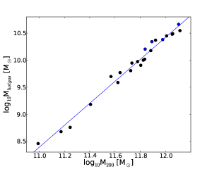
Figure 11.— Total hot gas mass inside r_vir = r₂₀₀ as function of total virial mass. Black dots: Simulations from GARROTXA run, their properties are presented in Tab. 2. Blue dots: Simulations outside GARROTXA run, parameters from these simulations are not presented in Tab. 2.

4.2.3 Total hot gas mass: are results from observations biased?

As previously mentioned it is challenging to infer the total hot gas mass in the MW by using the available observational data. Matter in the CGM is hot (T $=$ 10${}^{5}-$10⁷ K) and tenuous (n $\simeq$ 10${}^{-5}-$10^-4 cm^-3). Plasma in these conditions couples with radiation mainly through electronic transitions of elements (C, N, O) in their He-like and H-like ionization stages. The strongest of these transitions falling in the soft X-rays. Due to the extreme low densities and small optical length of the CGM, detection of the absorption/emission features produced by this material has proved particularly challenging with the still limited sensibility of the gratings on board Chandra and XMM-Newton. As a consequence, observations in only a few number of line of sight directions have been useful to observe X-ray absorption in quasar spectra. In this scenario it is clear that simulations can play an important role in the study of hot gas as they let us to explore the complexities in a simulated galactic systems. Including such information enable us to study how observational techniques can lead to biased results for the total hot gas in the galactic system.
With such aim we have located our mock observer at 8 kpc from the galactic center (i.e. similar to solar position) in the galactic plane and at a random azimuthal angle, inside our MW-sized simulations. For comparison we refer the reader to observations of OVII column densities presented in Gupta et al. (2012) and to total hot gas values they obtained. In Tab. 3 we show the results we have obtained when making observations to a similar number of randomly distributed directions into the sky as the ones in Gupta et al. (2012). As in our simulations we have not realistic chemical species like oxygen we have assumed that we are observing all hot gas, and present the column densities measured in each line of sight. As it is common in the literature (e.g. Gupta et al., 2012; Bregman & Lloyd-Davies, 2007), we have assumed a spherical uniform gas distribution for the hot gas halo. As a first attempt, we have estimated, from the column density values at each direction, the total galactic hot gas mass, assuming a path length of L = 239 kpc = r_vir. We have found that using the spherical uniform approach, the total hot gas mass is systematically overestimated (see Tab. 3 last column). This is a consequence of that the density distribution in our model is not uniform but it decreases as a power-law (see Fig. 5 and 12). However, this calculation is not very useful, as it requires an a-priori knowledge of the CGM path length (L) which is observationally unknown.

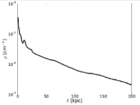
Figure 12.— Spherically averaged hot gas density (T $>$ 3$\times$10⁵ K) as function of radius for the model G.321 at z = 0.

A popular technique among observational studies (i.e. Gupta et al., 2012; Bregman & Lloyd-Davies, 2007) is to take advantage of the two observables for the hot gas in the CGM: the column density (N_H) and the emission measure (EM). This technique uses these two quantities to derive the total hot gas mass with no need of imposing an a-priori mean density or optical path length. We show results from using this technique in Tab. 4, both for the optical path length, the mean density and the total hot gas mass. In this case, as can be seen in the table, results show an underestimation of the total hot gas mass by factors $\sim$0.7$-$0.1, result that is independent on the observed direction. Again this result is a consequence of that the real density distribution of our model is not uniform but decreasing with radius as a power law.
As a conclusion we state that using both, column density plus imposed optical depth (independently of using the value from a single observation or the mean) or a combination of column density and emission measure, we are not able to obtain the real hot halo gas mass, when assuming it is isotropically distributed in the galactic halo. Nevertheless, these measurements, particularly the observational method in the literature using both N_H and EM are useful to get an order of magnitude estimate of the total hot gas mass of the halo. The work is in progress to find the density profile that will allow us to get the best hot halo gas mass estimation, from observations.

	l	b	NH	Mtotal,Hotgas
	[deg]	[deg]	[1019cm-2]	[1010 M⊙]
FoV1	179.83	65.03	2.59	4.57
FoV2	17.73	-52.25	1.31	2.31
FoV3	91.49	47.95	2.96	5.21
FoV4	35.97	-29.86	2.81	4.96
FoV5	289.95	64.36	2.62	4.62
FoV6	92.14	-25.34	2.06	3.63
FoV7	287.46	22.95	2.62	4.62
FoV8	40.27	-34.94	2.59	4.57

Table 3Mock observations of eight randomly distributed directions in the sky, in our G.321 simulation at z = 0. The total hot gas mass in the simulation, up to r_vir, is M_vir = 1.2$\times$10¹⁰ M_⊙. We have defined hot gas as gas at T $>$ 3$\times$10⁵ K. We have assumed L = 230.1 kpc = r_vir.

	EM	L	n	Mtotal,Hotgas
	[10-3cm-6 pc]	[kpc]	[10-4cm-3]	[1010 M⊙]
FoV1	2.03	40.2	2.2	0.11
FoV2	0.16	111.3	0.4	0.40
FoV3	1.58	53.7	1.7	0.21
FoV4	0.79	56.6	1.2	0.17
FoV5	0.89	80.5	1.1	0.42
FoV6	1.40	59.1	1.5	0.25
FoV7	0.98	74.1	1.1	0.36
FoV8	0.61	116.5	0.7	0.88

Table 4Emission Measure (EM) values from the same eight randomly distributed directions in the sky as in Tab. 3. Using EM and N_H values we have computed the path length (L) and hot gas volume density (n). Finally we show the total hot gas mass obtained when assuming a sphere with constant density (n) and its radius equal to the path length (L). The real total hot gas mass in the simulation is M_vir = 1.2$\times$10¹⁰ M_⊙.

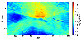
Figure 13.— Hot gas (T $>$ 3$\times$10⁵ K) column density (top) in a full sky view of simulation G.321 in galactic coordinates, at z = 0. All values have been computed as observed from R = 8 kpc and at an arbitrary azimuthal angle.

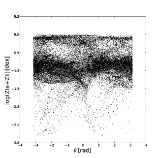
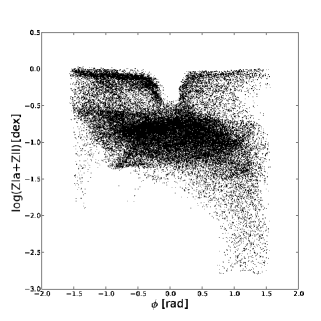
Figure 14.— Hot gas (T $>$ 3$\times$10⁵ K) view in spherical galactic coordinates of the G.321 model, at z = 0. Top: metallicity as function of the azimuthal angle. Bottom: metallicity as function of the vertical angle. ZIa and ZII are metals from SNe Ia and II, respectively. All values have been computed as observed from the galactic center.

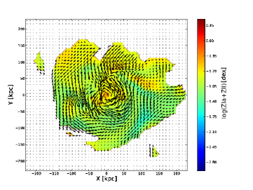
Figure 15.— Hot gas (T $>$ 3$\times$10⁵ K) projected metallicity (color map) and galactocentric velocity direction (arrows) in the principal plane X-Y of the G.321 model, at z=0. ZIa and ZII are metals from SNe Ia and II, respectively

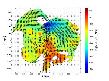
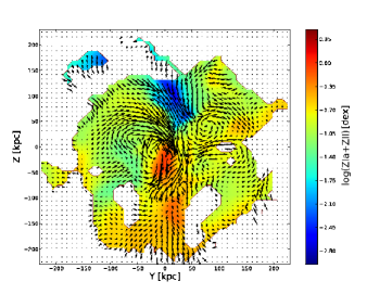
Figure 16.— Hot gas (T $>$ 3$\times$10⁵ K) projected metallicity (color map) and galactocentric velocity direction (arrows) in two principal planes, X-Z (top) and Y-Z (bottom) of the G.321 model, at z = 0. ZIa and ZII are metals from SNe Ia and II, respectively

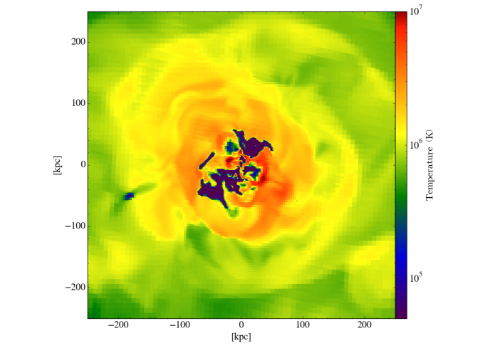
Figure 17.— Warm-hot gas slice plot at an arbitrary plane of the simulation G.323, at z = 0.

4.2.4 Total hot gas mass: accounting for the missing baryons

The baryonic fraction in our simulations corresponding only for stellar and cold gas mass, falls in between 0.084 and 0.096. These numbers are far from the cosmic baryon fraction F_b,U=0.171$\pm$0.009 (Dunkley et al., 2009; Planck Collaboration et al., 2014) but are comparable to reported values for isolated spiral galaxies based on weak lensing and stellar mass are 0.056 (Hoekstra et al., 2005). Such mismatch between cosmic and galaxy baryon budget suggests that either gas has escaped halos or never reached them and it and it is located in the Large Scale Structure warm-hot intergalactic (WHIM) gas (Cen & Ostriker, 1999) or that warm-hot gas embedded in dark matter halos may account at least for part of the missing baryons if not all. In our simulations the baryonic fraction reaches (0.107$-$0.120) even after adding the hot gas mass component inside halos. Because we do not include the feedback effect of an AGN, that may eject the gas outside the halo, we can consider our estimates as an upper limit to the halo hot gas mass. Based on the previous discussion we argue that the missing baryons must be placed both like hot gas mass inside dark matter halos (e.g. Gupta et al., 2012; Miller & Bregman, 2013b) and also in the IGM, along the filaments and far from the main galactic systems (Rasheed et al., 2010; Eckert et al., 2015). This is consistent with recent studies for CGIM in M31 (Lehner et al., 2015) as well as gas stripping in LMC (Salem et al., 2015).

5. Conclusions

In this paper we have introduced a new set of MW-sized cosmological N-body plus hydrodynamics simulations. Their resolution and realism are high enough to allow us to study stellar kinematics (Roca-Fàbrega et al., 2013, 2014) and evolution of large scale structures of these kind of galaxies. Most stellar disk parameters in our G.3 models are in agreement with observational ranges for the MW. Disk scale length and scale height as well as their dependence on the stellar age are reproduced. The simulated disk shows a large variety of large scale structures such us spiral arms, a ring and a bar. It also shows a flared and a warped configuration. The quality of our runs is comparable to the most recent works presented by Guedes et al. (2011) and Mollitor et al. (2015), a detailed comparison can be seen in Table LABEL:tab:1. Our simulations have a similar or a larger number of resolution elements (stellar particles or gas cells), higher spatial resolution, and a smaller mass per particle than the ones in those works. In addition, as we have shown in Fig. 4, our circular velocity curves are in a very good agreement with recent observations. On the other hand, a spheroid (bulge+halo) that is 2$-$3 times more massive than the one observed in the real MW is present in our G.3 models. Since the density of this spheroidal component is relatively low in the central region of our galactic systems it does not drive to centrally peaked circular velocity curves.

We have also analyzed the SFH in our simulations. We have found that our SFR values at z=0 are lower than recent observational values. Also the SFH peak in our G.3 models occurs at higher redshift than the one predicted by (Behroozi et al., 2013). In the most recent and realistic MW-sized simulations (Guedes et al., 2011; Mollitor et al., 2015; Bird et al., 2013), the predicted SFH is also not well reproduced. We have also found that total gas mass and its distribution in temperature slightly differ from MW observations. This mismatch in SFH and mass gas distribution is usual in simulations due to the lack of understanding of subgrid physics and to the difficulty of accounting for all physical processes involved in the formation and evolution of galaxies. Studies like ours will help to constrain such subgrid models. Recently, it has been proposed that the inclusion of a kinematic feedback might solve the early star formation issue and thus change the position of the SFH peak.

The work presented here is focused in the study of the distribution and the amount of potentially X-ray emitting gas (T $>$ 3$\times$10⁵ K) of our simulations. The comparison of the properties of the hot gas in our simulation with the observations of the hot halo X-ray corona of the MW and external galaxies was made by producing hot gas column density mock observations. Conclusions on this part follows:

• Hot gas is not distributed homogeneously around the galactic halo.

• There is no evidence of a hot gas thick disk in our models.

• By using the real mass of warm-hot gas in our simulations we conclude that about 53%$-$80% of the missing baryons can be accounted by hot gas in the halo corona. The exact value depends on the simulated galactic system (e.g. halo mass). We argue that the lacking baryons are placed in filaments (IGM), not inside main galactic systems, as preheated warm-hot gas (Rasheed et al., 2010). It is important to mention that in our simulations AGN feedback from a central galactic black hole has not been implemented. It is still open to debate how a relatively low mass black hole, as the one in the real MW, could affect the mass and temperature distribution of the hot halo gas and thus the SFH.

• Hot gas density follows several streams in the halo that can be detected because of their changes in kinematics and metallicity. We have seen how low metallicity streams come from the IGM while others with higher metallicity depart from the disk. We have also detected the infall of high metallicity gas that can be interpreted as coming from a satellite accretion.

• The total hot gas mass in the halo can not be recovered when assuming a spherical uniform gas distribution. In our model the real hot gas density distribution lead to an overestimation when using the mean column density plus a fixed optical depth under the spherical uniform assumption. On the other hand it drives to an underestimation of the total hot gas mass when we use the column density plus the emission measure when using the same assumption.

• Following previous works we have found that a clear relation exist between total hot gas mass and virial mass of halos. This result is important as it becomes new method to constrain the total mass of galactic systems, such as the Milky Way.

Appendix A Resolution study

In this appendix we show a test of numerical convergence using a low resolution resimulation of our main model. The resimulation presented here (G.321_lr) has been obtained using the same IC and initial parameters as in G.321 but with a resolution of 218 pc instead of 109 and $\sim$9$\times$10⁵ DM particles inside R_v instead of $\sim$7$\times$10⁶. In Fig.18 we show a comparison of the total, DM, stellar and gas circular velocity curves computed using $\sqrt{(}GM/r)$ as a proxy for V_c. We see that resolution does not affect the total circular velocity curve profiles. However, it is interesting to note that circular velocity curve from the G.321 gas component shows significantly higher V_c values at large radii. This result is in agreement with what was obtained by Scannapieco et al. (2012); i.e. the properties of the gaseous component seem to be the most sensitive to numerical resolution effects. We show in Tab.5 the values of the main parameters of the G.321 run and compare them with the corresponding ones of the G.321_lr model. We see that, aside from the mass of cold gas and related quantities, like SFR at z=0, most parameters do not differ from each other by ore than 30$\%$. This was also found in Scannapieco et al. (2012). From this result, we conclude that although, in general, parameters are not sensitive to changes in resolution, caution must be exercised when analyzing the cold gas component and the SFR. In addition, we notice that the cold gas fraction is not only sensitive to numerical resolution (the maximum refinement level) but also to changes in terms of number of cells (different aggressive refinement, see Sec.3.3). On the other hand, the difference observed in G.321 gas velocity curve at large radii is simply due to the fact that this run ends up with much more gas. Additional studies of numerical convergence of the code can be found in Avila-Reese et al. (2011); González-Samaniego et al. (2014).

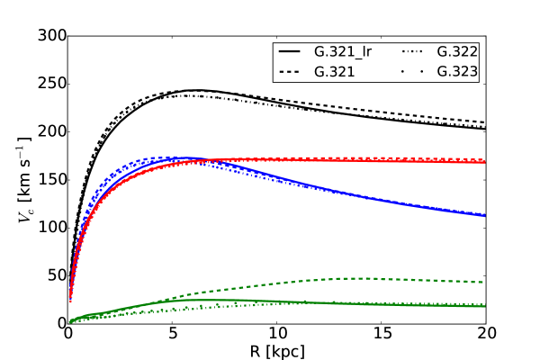
Figure 18.— Circular velocity curves of G.321, G.322, G.323 and G.321_lr computed using GM/r approximation (see Tab.5 for more details about models). Black: total, red: dark matter, blue: stars, green: gas.

	G.321	G.321_lr	$\mid$(G.321-G.321_lr)/G.321$\mid$$\times$100
Mvir [M⊙]	7.33$\times$1011	7.33$\times$1011	0.0
rvir [kpc]	230.1	230.5	0.2
M∗ [M⊙]	6.1$\times$1010	6.0$\times$1010	2.0
Mgas [M⊙]	2.70$\times$1010	1.93$\times$1010	28.5
Mhotgas [M⊙]	1.22$\times$1010	1.06$\times$1010	13.1
Mwarmgas [M⊙]	5.66$\times$109	7.33$\times$109	29.5
Mcoldgas [M⊙]	9.34$\times$109	1.37$\times$109	85.3
M200 [M⊙]	6.84$\times$1011	6.61$\times$1011	3.4
r200 [kpc]	175.6	175.6	0.0
Fb,U	0.120	0.108	10.0
c	28.5	25.4	10.9
Rd [kpc]	2.56 (4.89/2.21)	2.13 (4.2/1.8)	16.8
hz,young [pc]	277	390	40.7
hz,old [pc]	1356	1032	23.9
$\alpha_{X}$	-0.62	-0.60	3.2
SFR (z=0) [M⊙yr-1]	0.27	0.16	40.7
Vc⊙(R=8kpc) [kms-1]	239.8	239.2	0.3
Rpeak [kpc]	5.69	5.69	0.0
Vc(Rpeak) [kms-1]	243.8	243.6	0.1
V2.2/V200	1.90	1.87	1.6

Table 5Comparison between general parameters of GARROTXA original model G321 and low resolution run G321_lr. All parameters shown here have been well described in Tab.LABEL:tab:1.

Appendix B Jeans length

In this section, following the condition proposed by Truelove et al. (1997), we show that in our simulations the resolution is above the minimum that ensures the formation of stellar particles is of physical origin rather than numerical. In order to see this we have computed the local Jeans wavelength of the cold gas ($\lambda_{J}$) according to Eq.1.
In Fig.19 we show a histogram of the Jeans length in units of the size of the corresponding cell for simulation G322. Except for few ones, cells satisfy the Truelove criterium.

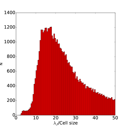
Figure 19.— Histogram of the cold gas (T$<$4$\times$10⁴) Jeans length computed following Eq.1, in units of the corresponding cell size, for simulation G322.

References

- Abadi et al. (2003) Abadi M. G., Navarro J. F., Steinmetz M., Eke V. R., 2003, ApJ, 591, 499
- Agertz & Kravtsov (2015) Agertz O., Kravtsov A. V., 2015, arXiv:1509.00853, ApJ, submitted
- Agertz et al. (2011) Agertz O., Teyssier R., Moore B., 2011, MNRAS, 410, 1391
- Anderson & Bregman (2010) Anderson M. E., Bregman J. N., 2010, ApJ, 714, 320
- Asplund et al. (2009) Asplund M., Grevesse N., Sauval A. J., Scott P., 2009, ARA&A, 47, 481
- Atanasijevic (1971) Atanasijevic I., ed. 1971, Selected exercises in galactic astronomy Vol. 26 of Astrophysics and Space Science Library
- Aumer et al. (2013) Aumer M., White S. D. M., Naab T., Scannapieco C., 2013, MNRAS, 434, 3142
- Avila-Reese et al. (2011) Avila-Reese V., Colín P., González-Samaniego A., et al. 2011, ApJ, 736, 134
- Baldry et al. (2008) Baldry I. K., Glazebrook K., Driver S. P., 2008, MNRAS, 388, 945
- Behroozi et al. (2013) Behroozi P. S., Wechsler R. H., Conroy C., 2013, ApJ, 770, 57
- Berkhuijsen (1998) Berkhuijsen E. M., 1998, in Breitschwerdt D., Freyberg M. J., Truemper J., eds, IAU Colloq. 166: The Local Bubble and Beyond Vol. 506 of Lecture Notes in Physics, Berlin Springer Verlag, The Volume Filling Factor of the WIM. pp 301–304
- Binney & Tremaine (2008) Binney J., Tremaine S., 2008, Galactic Dynamics: Second Edition. Princeton University Press
- Bird et al. (2013) Bird J. C., Kazantzidis S., Weinberg D. H., et al. 2013, ApJ, 773, 43
- Bogdán & Gilfanov (2011) Bogdán Á., Gilfanov M., 2011, MNRAS, 418, 1901
- Bovy et al. (2009) Bovy J., Hogg D. W., Rix H.-W., 2009, ApJ, 704, 1704
- Bovy & Rix (2013) Bovy J., Rix H.-W., 2013, ApJ, 779, 115
- Boylan-Kolchin et al. (2013) Boylan-Kolchin M., Bullock J. S., Sohn S. T., Besla G., van der Marel R. P., 2013, ApJ, 768, 140
- Boylan-Kolchin et al. (2009) Boylan-Kolchin M., Springel V., White S. D. M., Jenkins A., Lemson G., 2009, MNRAS, 398, 1150
- Bregman (2007) Bregman J. N., 2007, ARA&A, 45, 221
- Bregman & Lloyd-Davies (2007) Bregman J. N., Lloyd-Davies E. J., 2007, ApJ, 669, 990
- Brook et al. (2012) Brook C. B., Stinson G., Gibson B. K., et al. 2012, MNRAS, 419, 771
- Brooks et al. (2011) Brooks A. M., Solomon A. R., Governato F., et al. 2011, ApJ, 728, 51
- Bryan & Norman (1998) Bryan G. L., Norman M. L., 1998, ApJ, 495, 80
- Bullock et al. (2001) Bullock J. S., Dekel A., Kolatt T. S., et al. 2001, ApJ, 555, 240
- Cappi et al. (2013) Cappi M., Done C., Behar E., et al. 2013, arXiv:1306.2330, Supporting paper for the science theme, The Hot and Energetic Universe, to be implemented by the Athena+ X-ray observatory
- Cen & Ostriker (1999) Cen R., Ostriker J. P., 1999, ApJ, 514, 1
- Cen et al. (1990) Cen R. Y., Ostriker J. P., Jameson A., Liu F., 1990, ApJ, 362, L41
- Ceverino et al. (2010) Ceverino D., Dekel A., Bournaud F., 2010, MNRAS, 404, 2151
- Ceverino & Klypin (2009) Ceverino D., Klypin A., 2009, ApJ, 695, 292
- Chemin et al. (2015) Chemin L., Renaud F., Soubiran C., 2015, A&A, 578, A14
- Colín et al. (2010) Colín P., Avila-Reese V., Vázquez-Semadeni E., Valenzuela O., Ceverino D., 2010, ApJ, 713, 535
- Colín et al. (2013) Colín P., Vázquez-Semadeni E., Gómez G. C., 2013, MNRAS, 435, 1701
- Crain et al. (2010) Crain R. A., McCarthy I. G., Frenk C. S., Theuns T., Schaye J., 2010, MNRAS, 407, 1403
- Crain et al. (2013) Crain R. A., McCarthy I. G., Schaye J., Theuns T., Frenk C. S., 2013, MNRAS, 432, 3005
- Cuesta et al. (2008) Cuesta A. J., Prada F., Klypin A., Moles M., 2008, MNRAS, 389, 385
- Davé et al. (2001) Davé R., Cen R., Ostriker J. P., et al. 2001, ApJ, 552, 473
- Dekel & Birnboim (2006) Dekel A., Birnboim Y., 2006, MNRAS, 368, 2
- Dekel et al. (2009) Dekel A., Birnboim Y., Engel G., et al. 2009, Nature, 457, 451
- Du et al. (2006) Du C., Ma J., Wu Z., Zhou X., 2006, MNRAS, 372, 1304
- Dunkley et al. (2009) Dunkley J., Komatsu E., Nolta M. R., et al. 2009, ApJS, 180, 306
- Dutton et al. (2010) Dutton A. A., Conroy C., van den Bosch F. C., Prada F., More S., 2010, MNRAS, 407, 2
- Duval & Athanassoula (1983) Duval M. F., Athanassoula E., 1983, A&A, 121, 297
- Eckert et al. (2015) Eckert D., Jauzac M., Shan H., et al. 2015, Nature, 528, 105
- Evrard (1988) Evrard A. E., 1988, MNRAS, 235, 911
- Faerman et al. (2016) Faerman Y., Sternberg A., McKee C. F., 2016, arXiv:1602.00689
- Fall & Efstathiou (1980) Fall S. M., Efstathiou G., 1980, MNRAS, 193, 189
- Feldmann et al. (2011) Feldmann R., Carollo C. M., Mayer L., 2011, ApJ, 736, 88
- Feldmann et al. (2013) Feldmann R., Hooper D., Gnedin N. Y., 2013, ApJ, 763, 21
- Ferland et al. (1998) Ferland G. J., Korista K. T., Verner D. A., et al. 1998, PASP, 110, 761
- Ferrière (2001) Ferrière K. M., 2001, Reviews of Modern Physics, 73, 1031
- Flynn et al. (2006) Flynn C., Holmberg J., Portinari L., Fuchs B., Jahreiß H., 2006, MNRAS, 372, 1149
- Forero-Romero et al. (2011) Forero-Romero J. E., Hoffman Y., Yepes G., et al. 2011, MNRAS, 417, 1434
- Forman et al. (1985) Forman W., Jones C., Tucker W., 1985, ApJ, 293, 102
- Fukugita et al. (1998) Fukugita M., Hogan C. J., Peebles P. J. E., 1998, ApJ, 503, 518
- Georgakakis et al. (2013) Georgakakis A., Carrera F., Lanzuisi G., et al. 2013, arXiv:1306.2328, Supporting paper for the science theme, The Hot and Energetic Universe, to be implemented by the Athena+ X-ray observatory
- Gibbons et al. (2014) Gibbons S. L. J., Belokurov V., Evans N. W., 2014, MNRAS, 445, 3788
- Gnedin et al. (2009) Gnedin N. Y., Tassis K., Kravtsov A. V., 2009, ApJ, 697, 55
- González-Samaniego et al. (2014) González-Samaniego A., Colín P., Avila-Reese V., Rodríguez-Puebla A., Valenzuela O., 2014, ApJ, 785, 58
- González-Samaniego et al. (2014) González-Samaniego A., Vázquez-Semadeni E., González R. F., Kim J., 2014, MNRAS, 440, 2357
- Governato et al. (2010) Governato F., Brook C., Mayer L., et al. 2010, Nature, 463, 203
- Governato et al. (2004) Governato F., Mayer L., Wadsley J., et al. 2004, ApJ, 607, 688
- Governato et al. (2007) Governato F., Willman B., Mayer L., et al. 2007, MNRAS, 374, 1479
- Guedes et al. (2011) Guedes J., Callegari S., Madau P., Mayer L., 2011, ApJ, 742, 76
- Gupta et al. (2014) Gupta A., Mathur S., Galeazzi M., Krongold Y., 2014, APSS
- Gupta et al. (2012) Gupta A., Mathur S., Krongold Y., Nicastro F., Galeazzi M., 2012, ApJ, 756, L8
- Haardt & Madau (1996) Haardt F., Madau P., 1996, ApJ, 461, 20
- Hagihara et al. (2011) Hagihara T., Yamasaki N. Y., Mitsuda K., et al. 2011, PASJ, 63, 889
- Hagihara et al. (2010) Hagihara T., Yao Y., Yamasaki N. Y., et al. 2010, PASJ, 62, 723
- Hammer et al. (2007) Hammer F., Puech M., Chemin L., Flores H., Lehnert M. D., 2007, ApJ, 662, 322
- Hernquist & Katz (1989) Hernquist L., Katz N., 1989, ApJS, 70, 419
- Hernquist & Mihos (1995) Hernquist L., Mihos J. C., 1995, ApJ, 448, 41
- Hoekstra et al. (2005) Hoekstra H., Hsieh B. C., Yee H. K. C., Lin H., Gladders M. D., 2005, ApJ, 635, 73
- Hoyle (1953) Hoyle F., 1953, ApJ, 118, 513
- Hummels & Bryan (2012) Hummels C. B., Bryan G. L., 2012, ApJ, 749, 140
- Jurić et al. (2008) Jurić M., Ivezić Ž., Brooks A., et al. 2008, ApJ, 673, 864
- Kafle et al. (2012) Kafle P. R., Sharma S., Lewis G. F., Bland-Hawthorn J., 2012, ApJ, 761, 98
- Kafle et al. (2014) Kafle P. R., Sharma S., Lewis G. F., Bland-Hawthorn J., 2014, ApJ, 794, 59
- Kalberla et al. (2005) Kalberla P. M. W., Burton W. B., Hartmann D., et al. 2005, A&A, 440, 775
- Kaufmann et al. (2007) Kaufmann T., Mayer L., Wadsley J., Stadel J., Moore B., 2007, MNRAS, 375, 53
- Keller et al. (2015) Keller B. W., Wadsley J., Couchman H. M. P., 2015, MNRAS, 453, 3499
- Kereš et al. (2009) Kereš D., Katz N., Fardal M., Davé R., Weinberg D. H., 2009, MNRAS, 395, 160
- Kereš et al. (2005) Kereš D., Katz N., Weinberg D. H., Davé R., 2005, MNRAS, 363, 2
- Klypin & Holtzman (1997) Klypin A., Holtzman J., 1997, arXiv:astro-ph/9712217
- Klypin et al. (2001) Klypin A., Kravtsov A. V., Bullock J. S., Primack J. R., 2001, ApJ, 554, 903
- Klypin et al. (2002) Klypin A., Zhao H., Somerville R. S., 2002, ApJ, 573, 597
- Kolb & Turner (1990) Kolb E. W., Turner M. S., 1990, S&T, 80, 381
- Koposov et al. (2010) Koposov S. E., Rix H.-W., Hogg D. W., 2010, ApJ, 712, 260
- Kravtsov (2003) Kravtsov A. V., 2003, ApJ, 590, L1
- Kravtsov et al. (1997) Kravtsov A. V., Klypin A. A., Khokhlov A. M., 1997, ApJS, 111, 73
- Kravtsov et al. (2005) Kravtsov A. V., Nagai D., Vikhlinin A. A., 2005, ApJ, 625, 588
- Krumholz (2015) Krumholz M. R., 2015, in Vink J. S., ed., Astrophysics and Space Science Library Vol. 412 of Astrophysics and Space Science Library, The Formation of Very Massive Stars. p. 43
- Lehner et al. (2015) Lehner N., Howk J. C., Wakker B. P., 2015, ApJ, 804, 79
- Li et al. (2008) Li J.-T., Li Z., Wang Q. D., Irwin J. A., Rossa J., 2008, MNRAS, 390, 59
- Liang et al. (2016) Liang C. J., Kravtsov A. V., Agertz O., 2016, MNRAS, 458, 1164
- Licquia & Newman (2015) Licquia T. C., Newman J. A., 2015, ApJ, 806, 96
- López-Corredoira (2014) López-Corredoira M., 2014, A&A, 563, A128
- Maller & Dekel (2002) Maller A. H., Dekel A., 2002, MNRAS, 335, 487
- Marinacci et al. (2014) Marinacci F., Pakmor R., Springel V., 2014, MNRAS, 437, 1750
- Mathews & Brighenti (2003) Mathews W. G., Brighenti F., 2003, ARA&A, 41, 191
- Miller & Scalo (1979) Miller G. E., Scalo J. M., 1979, ApJS, 41, 513
- Miller & Bregman (2013a) Miller M. J., Bregman J. N., 2013a, ApJ, 770, 118
- Miller & Bregman (2013b) Miller M. J., Bregman J. N., 2013b, ApJ, 770, 118
- Mo & Mao (2004) Mo H. J., Mao S., 2004, MNRAS, 353, 829
- Mo et al. (1998) Mo H. J., Mao S., White S. D. M., 1998, MNRAS, 295, 319
- Mollitor et al. (2015) Mollitor P., Nezri E., Teyssier R., 2015, MNRAS, 447, 1353
- Moster et al. (2014) Moster B. P., Macciò A. V., Somerville R. S., 2014, MNRAS, 437, 1027
- Murante et al. (2015) Murante G., Monaco P., Borgani S., et al. 2015, MNRAS, 447, 178
- Navarro & Benz (1991) Navarro J. F., Benz W., 1991, ApJ, 380, 320
- Navarro & Steinmetz (2000) Navarro J. F., Steinmetz M., 2000, ApJ, 528, 607
- Navarro & White (1993) Navarro J. F., White S. D. M., 1993, MNRAS, 265, 271
- Okamoto et al. (2005) Okamoto T., Eke V. R., Frenk C. S., Jenkins A., 2005, MNRAS, 363, 1299
- Okamoto et al. (2003) Okamoto T., Jenkins A., Eke V. R., Quilis V., Frenk C. S., 2003, MNRAS, 345, 429
- Oman et al. (2015) Oman K. A., Navarro J. F., Fattahi A., et al. 2015, MNRAS, 452, 3650
- Peebles (1969) Peebles P. J. E., 1969, ApJ, 155, 393
- Pichardo et al. (2003) Pichardo B., Martos M., Moreno E., Espresate J., 2003, ApJ, 582, 230
- Piontek & Steinmetz (2011) Piontek F., Steinmetz M., 2011, MNRAS, 410, 2625
- Planck Collaboration et al. (2014) Planck Collaboration Ade P. A. R., Aghanim N., Armitage-Caplan C., et al. 2014, A&A, 571, A16
- Rasheed et al. (2010) Rasheed B., Bahcall N., Bode P., 2010, arXiv:1007.1980, PNAS, submitted
- Reid et al. (2014) Reid M. J., Menten K. M., Brunthaler A., et al. 2014, ApJ, 783, 130
- Robertson et al. (2004) Robertson B., Yoshida N., Springel V., Hernquist L., 2004, ApJ, 606, 32
- Robitaille & Whitney (2010) Robitaille T. P., Whitney B. A., 2010, ApJ, 710, L11
- Roca-Fàbrega et al. (2014) Roca-Fàbrega S., Antoja T., Figueras F., et al. 2014, MNRAS, 440, 1950
- Roca-Fàbrega et al. (2013) Roca-Fàbrega S., Valenzuela O., Figueras F., et al. 2013, MNRAS, 432, 2878
- Salem et al. (2015) Salem M., Besla G., Bryan G., et al. 2015, ApJ, 815, 77
- Santos-Santos et al. (2016) Santos-Santos I. M., Brook C. B., Stinson G., et al. 2016, MNRAS, 455, 476
- Savage et al. (2003) Savage B. D., Sembach K. R., Wakker B. P., et al. 2003, ApJS, 146, 125
- Scannapieco et al. (2015) Scannapieco C., Creasey P., Nuza S. E., et al. 2015, A&A, 577, A3
- Scannapieco et al. (2010) Scannapieco C., Gadotti D. A., Jonsson P., White S. D. M., 2010, MNRAS, 407, L41
- Scannapieco et al. (2012) Scannapieco C., Wadepuhl M., Parry O. H., et al. 2012, MNRAS, 423, 1726
- Scannapieco et al. (2009) Scannapieco C., White S. D. M., Springel V., Tissera P. B., 2009, MNRAS, 396, 696
- Scannapieco et al. (2011) Scannapieco C., White S. D. M., Springel V., Tissera P. B., 2011, MNRAS, 417, 154
- Shu (1991) Shu F., 1991, Physics of Astrophysics, Vol. II: Gas Dynamics. University Science Books
- Sofue et al. (2009) Sofue Y., Honma M., Omodaka T., 2009, PASJ, 61, 227
- Stinson et al. (2006) Stinson G., Seth A., Katz N., et al. 2006, MNRAS, 373, 1074
- Stinson et al. (2010) Stinson G. S., Bailin J., Couchman H., et al. 2010, MNRAS, 408, 812
- Stinson et al. (2013) Stinson G. S., Brook C., Macciò A. V., et al. 2013, MNRAS, 428, 129
- Toft et al. (2002) Toft S., Rasmussen J., Sommer-Larsen J., Pedersen K., 2002, MNRAS, 335, 799
- Truelove et al. (1997) Truelove J. K., Klein R. I., McKee C. F., et al. 1997, ApJ, 489, L179
- Trujillo-Gomez et al. (2015) Trujillo-Gomez S., Klypin A., Colín P., et al 2015, MNRAS, 446, 1140
- Valenti et al. (2016) Valenti E., Zoccali M., Gonzalez O. A., et al. 2016, A&A, 587, L6
- Vogelsberger et al. (2014) Vogelsberger M., Genel S., Springel V., et al. 2014, MNRAS, 444, 1518
- White & Frenk (1991) White S. D. M., Frenk C. S., 1991, ApJ, 379, 52
- White & Rees (1978) White S. D. M., Rees M. J., 1978, MNRAS, 183, 341
- Xue et al. (2008) Xue X. X., Rix H. W., Zhao G., et al. 2008, ApJ, 684, 1143
- Yao & Wang (2007) Yao Y., Wang Q. D., 2007, ApJ, 658, 1088
- Yoachim & Dalcanton (2006) Yoachim P., Dalcanton J. J., 2006, AJ, 131, 226
- Zemp (2014) Zemp M., 2014, ApJ, 792, 124