Real eigenvalues of non-Gaussian random matrices and their products

Abstract

We study the properties of the eigenvalues of real random matrices and their products. It is known that when the matrix elements are Gaussian-distributed independent random variables, the fraction of real eigenvalues tends to unity as the number of matrices in the product increases. Here we present numerical evidence that this phenomenon is robust with respect to the probability distribution of matrix elements, and is therefore a general property that merits detailed investigation. Since the elements of the product matrix are no longer distributed as those of the single matrix nor they remain independent random variables, we study the role of these two factors in detail. We study numerically the properties of the Hadamard (or Schur) product of matrices and also the product of matrices whose entries are independent but have the same marginal distribution as that of normal products of matrices, and find that under repeated multiplication, the probability of all eigenvalues to be real increases in both cases, but saturates to a constant below unity showing that the correlations amongst the matrix elements are responsible for the approach to one. To investigate the role of the non-normal nature of the probability distributions, we present a thorough analytical treatment of the $2\times 2$ single matrix for several standard distributions. Within the class of smooth distributions with zero mean and finite variance, our results indicate that the Gaussian distribution has the maximum probability of real eigenvalues, but the Cauchy distribution characterised by infinite variance is found to have a larger probability of real eigenvalues than the normal. We also find that for the two-dimensional single matrices, the probability of real eigenvalues lies in the range $[5/8,7/8]$.

I Introduction

The problem of the number of real roots of algebraic equations has a long history, but continues to attract attention, from the early works of Littlewood and Offord Littlewood and Offord (1939) to more recent developments Edelman and Kostlan (1995); Nguyen et al. (2014) (see the latter article for more related history and references). Mark Kac, in a seminal paper, proved that the expected number of real zeros of polynomials (of order $N$) whose coefficients are chosen from a normal distribution of zero mean is $\sim\frac{2}{\pi}\ln{N}$ Kac (1943). Others substantially extended these results and showed universality in that this is the leading order behavior, irrespective of the underlying distribution as long as they are zero-centered and have a finite variance Stevens (1969). Logan and Shepp Logan and Shepp (1966) studied the same when the coefficients are Cauchy distributed (and hence have infinite variance, and undefined average) the leading behavior goes as $c\ln N$, with $c\approx 0.7413$ which is larger than $2/\pi\approx 0.6366$, and hence there are more real zeros in the Cauchy case than when the variance is finite. Thus, the number of real roots of a random polynomial are generally quite small.

More recently, several works have explored the fraction of real eigenvalues for $n\times n$ matrices drawn from the real Ginibre ensemble. This ensemble consists of matrices whose elements are independently drawn from a normal distribution such as $N(0,1)$. For such matrices, it has been shown analytically that the expected number of real eigenvalues $E_{n}$ and the probability that all eigenvalues are real $P_{n,n}$ are given by Edelman et al. (1994); Edelman (1997); Kanzieper and Akemann (2005)

$$\lim_{n\to\infty}\frac{E_{n}}{\sqrt{n}}=\sqrt{\frac{2}{\pi}},\;\;P_{n,n}=2^{-n(n-1)/4}.$$ (1)

Thus the probability that all eigenvalues are real tends to zero as the matrix dimension increases, although the expected number of them increases algebraically.

Products of random matrices have also been studied, at least, since the classic work of Furstenberg and Kesten Furstenberg and Kesten (1960) (see, Bougerol and Lacroix (1985); Crisanti et al. (1993) for a discussion of subsequent work and some applications). The study of the spectra and singular values of the products of random matrices is currently a very active area of research Roga et al. (2011); Burda et al. (2012), and recent progress has been reviewed in Akemann and Ipsen (2015). When studying a problem related to the measure of “optimally entangled” states of two qubits Shuddhodan et al. (2011), the problem of the number of real eigenvalues of a product of matrices came up. It was shown in Lakshminarayan (2013) that the probability of all eigenvalues being real for the product of two, $2\times 2$ matrices from the real Ginibre ensemble is $\pi/4$. Somewhat surprisingly then there is a lesser probability that all eigenvalues are real for a single matrix ($1/\sqrt{2}$, from Eq. (1)) than for a product of two. This observation motivated numerical explorations in Lakshminarayan (2013) which showed that this probability tends to $1$ as the number of matrices in the product increases. Numerical results showing that this is true for higher dimensions was also discussed therein. This result has been proven analytically by Forrester Forrester (2014), who calculated $P_{n,n}$ explicitly in terms of Meijer G-functions for square matrices, and generalised by Ipsen Ipsen (2015) to rectangular matrices.

Most of the previous works on the properties of the eigenvalues have studied Gaussian matrices with independent, identically distributed (i.i.d.) entries. Exceptionally, Edelman, Kostlan and Shub Edelman et al. (1994) presented some numerical results indicating universality for the expected value $E_{n}$ of real eigenvalues of $n\times n$ real matrices. However, to the best of our knowledge, there is no study exploring such extensions to the products of matrices. Thus, two conditions are relaxed: first, non-Gaussian i.i.d. elements are taken as entries of the matrices, and second, we consider products of such independent matrices. In this case, the entries of the product matrix are naturally correlated in a complex manner and their distribution is, in general, anyway non-Gaussian.

Motivations for studying products of random matrices are well known in physics, and range from the study of localization in random media where transfer matrices are multiplied to dynamical systems where products of local stability matrices determine the Lyapunov exponents Crisanti et al. (1993). Applications for counting number of real eigenvalues of random matrices, especially of products, is of more recent provenance. The real eigenvalues of a class of random matrices indicate topologically protected level crossings at the Fermi energy in the bound states of a Josephson junction Beenakker et al. (2013). While the relevant object is a single matrix and not a product, it is conceivable that this provides a context for further investigation. In the context of entanglement of two qubits Lakshminarayan (2013), the real eigenvalues of products of two matrices were relevant in finding the measure of optimally entangled states Shuddhodan et al. (2011). Different distributions of matrix elements would result in different sampling of states on the Hilbert space. Finally, it is worth pointing out that the fact that real eigenvalues dominate the spectrum of products of matrices implies that generic orbits of dynamical systems are not of the complex unstable variety. Complex instability can occur in Hamiltonian systems with more than two degrees of freedom Contopoulos et al. (1994), when exponential instability is combined with rotational action in phase space. However, as a consequence of discussions in this paper, it seems unlikely that they would generically arise for long orbits, as they depend on eigenvalues of products of Jacobian matrices being complex.

To begin with, we ask: how do non-normal distributions affect the probability of real eigenvalues of a single matrix? In fact, a major part of this paper is concerned simply with $2\times 2$ matrices and various families of the distributions of matrix elements, and the probability that the eigenvalues are real is calculated exactly in many cases in Sec. II. In particular, we find the lower and upper bounds on the probability that both eigenvalues are real. In the family of symmetrized Gamma distributions, the range of probabilities is shown to be $[5/8,7/8]$. The upper bound is associated with the case when the matrix elements have a large weight at the origin and the lower bound in the opposite case when the maximum is away from the origin. In fact, these same bounds are obtained in a class of truncated distributions thus indicating that the probability of real eigenvalues depends crucially on whether the distributions are concentrated near the origin or away from it. The lower bound of $5/8$ is shown to be a tight one by proving this in general. The upper bound of $7/8$ still remains specific to these distributions, however we do believe that this is widely applicable as well.

We also find that the other features of the distributions of the matrix elements that play a significant role in determining the probability of real eigenvalues are the degree of smoothness and the existence of finite moments. It is noteworthy that these (apart from zero mean) are also the crucial features for universality in the case of random polynomials Edelman and Kostlan (1995). Given that the distributions are smooth and have finite moments, we tentatively propose that the normal distribution is the one with the maximum probability of finding real eigenvalues. If true, this provides a further unique characterization of the normal.

Besides the bounds, we also observe a hierarchy for the fraction of real eigenvalues for matrices constructed from these distributions. Specifically, for some commonly occurring distributions, we find that the eigenvalues are more real when the matrix elements are chosen from Cauchy distribution than Laplace, Gaussian or uniform distributions, which are arranged in the increasing order of the decay. However, we must mention that such hierarchy patterns are not simply determined by the tail behavior of the distribution, and the trends appear to be more complex as explained in the following section.

In Sec. III, we numerically study the properties of the eigenvalues of the matrix obtained after taking product of several matrices, and find that the increase in the probability to one holds for several other distributions. In particular, we explore the zero-centered uniform distribution, the symmetric exponential (Laplace) distribution and Cauchy distribution, as simple representative ones. The hierarchy mentioned above is seen to hold even after the multiplication of independent random matrices. The expected number of real eigenvalues is also studied which tends to the matrix dimension exponentially fast (with the number of matrices in the product), although the rate of approach is distribution-dependent.

It is unclear as to why the eigenvalues tend to become real when multiplying random structureless matrices. In an attempt at seeing how much this has to do with the act of multiplication, we study numerically the probability of real eigenvalues in the case of Hadamard (or Schur) products where the elements are simply the products of the corresponding elements of the multiplying matrices. Of course, in this case, the matrix elements remain uncorrelated. We find numerically that the probability of real eigenvalues increases with the number of matrices in the product, but tends to saturate at a value smaller than $1$. Numerical evidence that this approach is a power law is also provided. This then highlights that the correlations built up in the process of (usual) matrix multiplication are responsible for the phenomenon that the fraction of real eigenvalues tends to one.

II Real eigenvalues of a single $2\times 2$ matrix

Let $P_{n,k}^{(K)}$ denote the probability that a product of $K$ $n\times n$ random matrices has $k$ real eigenvalues. In this section, we study the simplest case, viz., the probability $P_{2,2}^{(1)}$ that all the eigenvalues of a $2\times 2$ matrix are real. We assume that the matrix elements are i.i.d. random variables chosen from the distribution $p(x)$ with support on the interval $[-u,u]$, where $u$ is finite for bounded distributions and infinity for unbounded ones, and that the distribution $p(x)$ is symmetric about the origin as a result of which the mean of the probability distribution is guaranteed to be zero. We first give analytical results for the probability $P_{2,2}^{(1)}$, which we study for many probability distributions, and then present some numerical results for the more general quantity $P_{n,k}^{(K)}$ in the following section.

Consider a $2\times 2$ matrix with i.i.d. elements defined as

$\left[\begin{array}[]{cccc}v&x\\ y&w\end{array}\right].$

As the discriminant $\mbox{tr}^{2}-4\det$ must be nonnegative for real eigenvalues, the probability that all eigenvalues are real is

$$\begin{split}P_{2,2}^{(1)}=\int^{u}_{-u}\int^{u}_{-u}\int^{u}_{-u}\int^{u}_{-u}\Theta\left[(v-w)^{2}+4xy\right]~{}p(v)p(w)p(x)p(y)~{}dvdwdxdy.\end{split}$$ (2)

Let the probability distribution of $z=v-w$ be $q(z)$ with $-2u\leq z\leq 2u$. Observe then that the probability of real eigenvalues can be written as

$$P_{2,2}^{(1)}=\frac{1}{2}+4\int^{0}_{-u}dx\int^{u}_{0}dy\int^{2u}_{0}dz~{}q(z)p(x)p(y)\Theta\left[z^{2}+4xy\right].$$ (3)

Here the even symmetry of the distributions is used, and also that when the signs of both $x$ and $y$ are the same, the constraint imposed by the Heaviside function is trivially satisfied. In the above equation, the distribution $q(z)$ is given by the convolution

$$q(z)=\int_{-u}^{u}~{}p(v)~{}p(w)~{}\delta(z-(v-w))~{}dvdw=\int_{-u}^{u}~{}p(v)p(v-z)~{}dv.$$ (4)

We note that this is indeed the usual convolution with $z\rightarrow-z$ due to the symmetry of $p(x)$. If $z\in[-2u,2u]$ the above expression for $q(z)$ is valid, else it is zero.

Equation (3) shows that the probability of both eigenvalues being real is at least one half for any probability distribution. The integral in Eq. (3) can be simplified if we use the convolution as

$$P_{2,2}^{(1)}=\frac{1}{2}+4\int^{u}_{0}dx\int^{u}_{0}dy\int^{2u}_{2\sqrt{xy}}dz~{}q(z)p(x)p(y)=1-4\int^{u}_{0}dx\int^{u}_{0}dy\int_{0}^{2\sqrt{xy}}dz~{}q(z)p(x)p(y).$$ (5)

The last equality follows from the fact that the convolution is itself a symmetric normalized distribution as $\int_{-\infty}^{\infty}q(z)dz=1$. Thus the evaluation of the probability of real eigenvalues reduces to evaluating the triple integral above.

It is also useful to write the distribution $q(z)$ as

$$q(z)=\frac{1}{2\pi}\int_{-\infty}^{\infty}dk~{}e^{ikz}~{}|{\tilde{p}}(k)|^{2},\;\;{\tilde{p}}(k)=\int_{-u}^{u}p(x)~{}e^{-ikx}~{}dx.$$ (6)

Here ${\tilde{p}}(k)$ is the characteristic function (or Fourier transform) of the probability distribution $p(x)$. Next consider the integral defined as

$$I(\alpha)=\int^{0}_{-u}dx\int^{u}_{0}dy\int^{2u}_{0}dz~{}q(z)p(x)p(y)\Theta\left[z^{2}+\alpha xy\right].$$ (7)

The value of interest is $I(4)$. Towards this end, differentiating $I(\alpha)$ with respect to (w.r.t.) $\alpha$, and performing the integral over the resulting delta function leads to

$$\frac{\partial I}{\partial\alpha}=\int^{\infty}_{-\infty}d\omega\int^{u}_{0}dx\int^{u}_{0}dy\frac{xy}{2\sqrt{\alpha xy}}\frac{\left|{\tilde{p}}(\omega)\right|^{2}}{2\pi}e^{i\omega\sqrt{\alpha xy}}p(x)p(y),$$ (8)

where ${\tilde{p}}(\omega)$ is given by Eq. (6). Noting that the above equation is valid only for $\alpha\in(0,4)$, we integrate the last expression w.r.t. $\alpha$ from $0$ to $4$, and use $I(0)=1/8$ to get $I(4)$ and finally the probability that both the eigenvalues are real as

$$P_{2,2}^{(1)}=1-\frac{4}{\pi}\int^{\infty}_{0}d\omega\int^{u}_{0}dx\int^{u}_{0}dy\left|{\tilde{p}}(\omega)\right|^{2}\frac{\sin(2\omega\sqrt{xy})}{\omega}p(x)p(y).$$ (9)

Below we will apply the result in either Eq. (5) or Eq. (9) to various choices of distribution $p(x)$. Before turning to explicit calculations, we note that the unbounded distributions have the following scale invariance property. Consider a division of the random matrix elements by a nonzero constant $b$. If $x^{\prime}=x/b$, then $\int_{-u^{\prime}}^{u^{\prime}}dx^{\prime}p^{\prime}(x^{\prime})=1$ where $p^{\prime}(x^{\prime})=bp(x)$ and $u^{\prime}=u/b$. From Eq. (2), it is seen that the probability $P_{2,2}^{(1)}$ is not affected by this scaling for unbounded functions, but for bounded ones, the limits should be redefined. While the above is an elementary analysis, we are not aware of it being discussed before.

Under conditions of smoothness (in the sense that all the derivatives exist at least in intervals) and symmetry of $p(x)$, it is interesting to enquire about the maximum value or upper bounds of $P_{2,2}^{(1)}$, for instance. For the lower bound, we have already stated that the probability of all real eigenvalues is at least one half. A tighter lower bound is however $5/8$, a proof of which was suggested to us by an anonymous referee which we discuss now. The probability of eigenvalues being real is

$$\mathbb{P}[(v-w)^{2}+4xy>0]=\frac{1}{2}\mathbb{P}[(v-w)^{2}+4xy>0|xy>0]+\frac{1}{2}\mathbb{P}[(v-w)^{2}+4xy>0|xy<0],$$ (10)

where the factors of $1/2$ arise as probability that $xy>0$ or otherwise. However the first conditional probability is $1$, and therefore

$$\mathbb{P}\left[(v-w)^{2}+4xy>0\right] = \frac{1}{2}+\frac{1}{2}\mathbb{P}[(v-w)^{2}-4xy>0|xy>0]$$

$$= \frac{1}{2}+\frac{1}{4}\mathbb{P}[(v+w)^{2}-4vw-4xy>0|xy>0,vw>0]$$

$$+ \frac{1}{4}\mathbb{P}[(v+w)^{2}-4vw-4xy>0|xy>0,vw<0]$$

$$= \frac{1}{2}+\frac{1}{4}\mathbb{P}[(v+w)^{2}-4vw-4xy>0|xy>0,vw>0]$$

$$+ \frac{1}{8}\mathbb{P}[(v+w)^{2}-4vw-4xy>0|xy>0,vw<0,|vw|<xy]+\frac{1}{8}$$ (13)

$$\geq \frac{5}{8}.$$ (14)

Here, in the second equality, further conditions on the sign of $vw$ are used with equal probabilities for either occurrence (from the symmetry and independence of the distributions). In the third equality, a further certainty is carved out by using the possibility that when $|vw|>xy>0$ (occurence probability being $1/2$), the discriminant is certainly positive. However our attempts at a similar approach for the upper bound were not successful.

Although one can obtain get some insight into the bounds, for what kind of distributions these bounds actually occur is discussed below.

II.1 Bounded distributions

II.1.1 Symmetric Beta distribution

Consider the symmetric Beta distribution with zero mean defined as

$$p_{\mu,\nu}(x)=\frac{\Gamma(\mu+\nu+2)}{2\Gamma(1+\mu)\Gamma(1+\nu)}~{}(1-|x|)^{\mu}~{}|x|^{\nu}~{},~{}\mu,\nu>-1$$ (15)

with support on the interval $[-1,1]$. This is a two-parameter symmetric family which can be nonsmooth at $x=0$. For $\mu=\nu=0$, the above distribution reduces to a uniform distribution, while $\mu=1,\nu=0$ and $\mu=0,\nu=1$ correspond to tent-shaped or V-shaped distribution respectively.

Case: ${\mathbf{\mu}=0}$

Distribution $p_{0,\nu}(x)\sim|x|^{\nu}$	Probability $P_{2,2}^{(1)}$
$\nu=-4095/4096$	0.874959
$\nu=-7/8$	0.849868
$\nu=-1/2$	0.759836
$\nu=0$	0.680556
$\nu=1$	0.63709
$\nu=3/2$	0.632888
$\nu=2$	0.631023
$\nu=3$	0.62928
$\nu=4$	0.628361
$\nu=200$	0.625078
$\nu=400$	0.625039

Table 1: Probability that both eigenvalues are real for a $2\times 2$ matrix with matrix elements chosen independently from the distribution in Eq. (15), with $\mu=0$. As $\nu$ approaches $-1$, the probability seems to limit to $7/8$, while for $\nu\to\infty$, it tends to $5/8$ (see text for details).

For the uniform distribution, the convolution $q(z)=(2-|z|)/4$ on $[-2,2]$ and zero elsewhere. Using Eq. (5), we find that

$$P_{2,2}^{(1)}(\nu=0)=\frac{1}{2}+\int_{0}^{1}dx\int^{1}_{0}dy\int^{2}_{\sqrt{4xy}}dz~{}q(z)=\frac{49}{72}=0.680556.$$ (16)

Thus the uniform distribution results in a smaller fraction of real eigenvalues when compared to the normal distribution Edelman et al. (1994), but not by very much.

When $\mu=0$ and $\nu$ is nonzero and positive, the distribution $p_{0,\nu}(x)\sim|x|^{\nu}\Theta(1-|x|)$ is zero at the origin. As $\nu$ tends to infinity, the weight of the distribution gets increasingly concentrated at $\pm 1$ and as Table 1 shows, the probability of real eigenvalues decreases. The distribution is smooth when $\nu=2k$ is an even integer. In this case, an analytical expression is possible for arbitrary $k$, and given by Eq. (38) of Appendix A. Numerical analysis of Eq. (38) for large $\nu$ strongly suggests that

$$P^{(1)}_{2,2}(0,\nu)=\frac{5}{8}+{\cal O}(\nu^{-1}),\;\;\nu\gg 1.$$ (17)

An insight into the above result can be gained by the following heuristic arguments: If we consider the limiting distribution as the Bernoulli ensemble with only two choices of entries $\pm 1$ with equal probabilities, we get only $16$ matrices in the ensemble of which $12$ have real eigenvalues. Thus it would seem that the ratio should have converged to $12/16=3/4$. However, there are $4$ cases where both the eigenvalues are exactly zero. If we believe that in the case of continuous distributions these are modified into cases with real and complex eigenvalues and equally, we get $6$ cases of complex values and the fraction is consistent with $5/8$ for real eigenvalues. Another related heuristic argument, closer to the continuous distributions under consideration, starts with the distribution

$$p(x)=\frac{1}{2}(\delta(x+1)+\delta(x-1)),$$ (18)

and applies Eq. (9) with $\tilde{p}(\omega)=\cos(\omega)$, leading to

$$P^{(1)}_{2,2}=1-\frac{2}{\pi}\int_{0}^{\infty}\dfrac{\sin\omega\cos^{3}\omega}{\omega}\,d\omega=\frac{5}{8}.$$

A proof of the assertion in Eq. (17) by analysing the double sums in Eq. (38) seems rather difficult to obtain, but it is possible to tackle the Gamma distribution given by Eq. (24), for which also the probability $p(x)$ is zero at the origin and increases algebraically away from it, and show that indeed the limit probability is $5/8$, see Sec. II.2.2. Thus the lower bound derived above is a tight one.

We now turn to the case when $-1<\nu<0$ where the probability distribution $p_{0,\nu}$ piles up at the origin. As shown in Table 1, the probability of real eigenvalues increases as $\nu$ decreases towards $-1$. It is obvious that if the matrix elements are chosen from a Dirac-delta distribution centred about zero, both the eigenvalues are definitely real. But whether the probability limits to something less than one as $\nu$ approaches $-1$ is of natural interest. As shown in Appendix A, we find that

$$P_{2,2}^{(1)}(0,\nu)=\frac{7}{8}-{\cal O}(1+\nu),~{}~{}\nu\to-1.$$ (19)

Thus it is interesting that the distribution $\sim|x|^{\nu}$ restricted to an interval spans a range of behaviors for the probability of real eigenvalues. As the matrix elements probability gets increasingly piled up at the ends ($\pm 1$), the probability of real eigenvalues decreases and tends to $5/8$, while in the opposite case when the elements are piled up around origin, the probability approaches the maximum value of $7/8$.

Case: $\mathbf{\nu}=0$

Distribution $p_{\mu,0}(x)\sim(1-|x|)^{\mu}$	Probability $P_{2,2}^{(1)}$
$\mu=-1/2$	0.654534
$\mu=1/2$	0.695759
$\mu=3/4$	0.70085
$\mu=1$	0.704854

Table 2: Probability that both eigenvalues are real for a $2\times 2$ matrix with matrix elements chosen independently from the distribution in Eq. (15) with $\nu=0$. The probability lies in the interval [$5/8,11/15$] for $\mu\in(-1,\infty)$.

For $\nu=0$, the probability distribution $p_{\mu,\nu}(0)\neq 0$ and we find that with increasing $\mu$, the probability that the eigenvalues are real increases, refer Table 2. Partial analytical results are possible. For example, for the case when $\mu=1,\nu=0$ (“tent” distribution), the convolution is

$$q(z)=\left\{\begin{array}[]{ll}\frac{1}{6}(2-|z|)^{3}&1\leq|z|\leq 2\\ \frac{1}{6}(4-6|z|^{2}+3|z|^{3})&0\leq|z|\leq 1.\end{array}\right..$$ (20)

The resulting integral in Eq. (5) can now be done using hyperbolic coordinates. This results in

$$P_{2,2}^{(1)}(\mu=1,\nu=0)=\frac{16143}{22400}-\frac{23\ln 2}{1008}\approx 0.704854.$$ (21)

It is reasonable to expect that as $\mu$ increases (and $\nu=0$), the probability increases to that when the elements are distributed according to the Laplace distribution $\sim\exp(-|x|)$ which is obtained as $\mu\rightarrow\infty$. We will deal with the Laplace distribution below, but state here that the probability of real eigenvalues in this case is $11/15\approx 0.733$. However, for negative $\mu$ where the matrix elements have a tendency to be close to $\pm 1$, from the discussion in the last subsection, we expect the probability to approach $5/8$ as $\mu\to-1$. Thus for the distribution $p_{\mu,0}(x)$, the probability of real eigenvalues lies in the range $\left[5/8,11/15\right]$.

II.1.2 A smooth family

Consider another class of smooth zero mean distributions bounded on the interval $[-1,1]$ defined as

$$p_{\eta}(x)=\dfrac{\Gamma(\eta+\frac{3}{2})}{\sqrt{\pi}\Gamma(\eta+1)}(1-x^{2})^{\eta}~{},~{}\eta>-1.$$ (22)

Of course, for $\eta>0$, the distribution is continuous but not smooth at $\pm 1$, but this does not seem crucial. When $\eta=0$, $p_{\eta}(x)$ is uniform on the said interval, and as $\eta\rightarrow\infty$ the distribution approaches the normal distribution with the variance scaling as $1/\eta$. As discussed above, the probability of real eigenvalues is independent of the variance and therefore, we expect that the large $\eta$ value for this probability will coincide with the known result for the normal distribution, namely, $1/\sqrt{2}\approx 0.707\cdots$ Edelman et al. (1994) (also, see Sec. II.2.1). The probability of real eigenvalues is calculated for some values of integer $\eta$ in Appendix B, and we find that the probability indeed approaches $1/\sqrt{2}$ with increasing $\eta$.

When $\eta$ is negative, the distribution $p(x)$ diverges at $x=\pm 1$, and from the discussion in the preceding subsection, we expect the probability of having real eigenvalues to approach $5/8$ as $\eta\to-1$. The case of $\eta=-1/2$ is that of the arcsine distribution. The convolution with itself can be found and is a complete Elliptic integral. However, even if further analytic results seem to be hard, this enables a more accurate numerical estimate of the probability of real eigenvalues which is $\approx 0.662$. Further decreasing $\eta$ makes the numerical evaluation unstable, but results indicate a monotonic decrease in the probability.

II.2 Distributions with infinite support

II.2.1 Gaussian

The case of normal or Gaussian distribution is the most studied and there are general results Edelman et al. (1994); Lakshminarayan (2013); Forrester (2014). We consider a zero centered, unit variance Gaussian distribution for the matrix elements given by

$$p(x)=\frac{e^{-x^{2}/2}}{\sqrt{2\pi}};\;x\in(-\infty,\infty).$$ (23)

The probability of both eigenvalues being real has already been shown, using Eq. (9), to be exactly equal to $1/\sqrt{2}$ in Lakshminarayan (2013), and alternative derivations naturally exist, see the works of Edelman (Edelman et al., 1994) and Forrester Forrester (2014). However to place it in the context of this paper, we rederive the probability of real eigenvalues in this case in Appendix C.

It is well known that the normal or Gaussian distribution is singled out in numerous ways, for example, as one that maximizes entropy for a given mean and variance, or as the limit of sums of random variables. In the context of the present work, it seems plausible that the normal distribution is once again to be singled out as the distribution of matrix elements that maximizes the probability of finding real eigenvalues among the class of smooth, symmetric, and finite moments distributions. To test this further, we have looked at distributions $p(x)$ such as $\sim\exp(-x^{4})$, $\sim\exp(-x^{2}-rx^{4})$ ($r>0)$ etc. and verified in all these cases that the probability of real eigenvalues is indeed less than $1/\sqrt{2}$. We advance this proposition tentatively based on evidence gathered so far, and from results to be presented below.

II.2.2 Gamma distribution

We next consider the symmetrized Gamma distribution defined as

$$p_{\gamma}(x)=\frac{1}{2\Gamma(\gamma)}|x|^{\gamma-1}e^{-|x|}~{},~{}\gamma>0.$$ (24)

where the scale for the exponential decay has been set to one. The special case of Laplace distribution for which $\gamma=1$ and the general case using the convolution route are discussed in Appendix  D. The convolution itself is given by

$$q(z)=\dfrac{1}{4\Gamma(2\gamma)}e^{-|z|}|z|^{2\gamma-1}+\dfrac{1}{2^{\gamma+\frac{1}{2}}\sqrt{\pi}\Gamma(\gamma)}|z|^{\gamma-\frac{1}{2}}K_{\gamma-\frac{1}{2}}(|z|),$$ (25)

where $K_{\nu}(z)$ is the modified Bessel function of the second kind DLMF . The results obtained by analysing the resulting integrals are shown in Table 3, and we find that with increasing $\gamma$, as the weight of the distribution at the origin decreases, the probability $P_{2,2}^{(1)}$ also decreases.

The behavior of the probability of real eigenvalues as $\gamma$ approaches zero can be understood as follows. As $\gamma$ approaches zero from the positive side, the distribution and both the terms in the convolution $q(z)$ diverge at the origin as $1/|z|$. The latter can be seen as $K_{-1/2}(z)=K_{1/2}(z)=\sqrt{\pi/2}e^{-z}/\sqrt{z}$, and $\lim_{z\rightarrow 0}\Gamma(2z)/\Gamma(z)=1/2$, as follows from the duplication formula for the Gamma function Abramowitz and Stegun (1964). Since we expect that the divergence at the origin is all that matters, the probability for real eigenvalues will converge to the case of the bounded distribution $|x|^{\nu}$ already studied above, and therefore the probability for real eigenvalues increases to $7/8$ as $\gamma\to 0$.

For increasing $\gamma>1$, the distribution itself is peaked away from the origin and has two symmetric maxima at $\sim\gamma$. The probability $P_{2,2}^{(1)}(\gamma)$ now decreases from the $\gamma=1$ value and monotonically seems to approach $5/8$, the lower limit for the bounded $|x|^{\nu}$ distributions as $\nu$ increased. Indeed the piling up of the probability of the matrix elements at two symmetric “walls” makes this plausible. To analyze this further, we restrict attention to integer values of $\gamma$ and give an exact evaluation in terms of finite sums as

$$P_{2,2}^{(1)}(\gamma)=\frac{1}{2}+A_{1}(\gamma)+A_{2}(\gamma),$$ (26)

where $A_{1}$ and $A_{2}$ are given by Eq. (62) and originate from the first and second terms of the convolution $q(z)$ in Eq. (25) respectively. To find the limiting value for the probability of real eigenvalues for large $\gamma$, we note that like the distribution $p_{\gamma}(x)$, the first term in the convolution $q(z)$ is also peaked around $z\sim\pm 2\gamma$, but the second term peaks at $z=0$ so that the two terms in the convolution have practically disjoint supports. As a consequence, for large $\gamma$, the dominant contribution to the probability in Eq. (26) comes from $A_{1}(\gamma)$ which represents the overlap between the distribution and the convolution, and $A_{2}(\gamma)$ can be neglected. As discussed in Appendix D, on analysing the sum $A_{1}(\gamma)$, we get

$$P^{(1)}_{2,2}(\gamma)=\frac{5}{8}+\frac{1}{16\sqrt{2\pi\gamma}}+{\cal O}(\gamma^{-1}),\;\;\gamma\gg 1.$$ (27)

In summary, for the symmetrized Gamma distributions, the probability of real eigenvalues also seems to be in the range $[5/8,7/8]$. The distribution having a nonanalyticity at the origin leads to larger probability for real eigenvalues compared to the normal distribution and it seems comparable to the bounded power law distributions $|x|^{\nu}$ studied above except in the rates of convergence.

Distribution symmetric Gamma	Probability $P_{2,2}^{(1)}$
$\gamma=1/4$	0.824051
$\gamma=1/2$	0.784155
$\gamma=1$	0.733333
$\gamma=2$	0.68325
$\gamma=3$	0.660393
$\gamma=10$	0.633238
$\gamma=100$	0.627494

Table 3: Probability that both eigenvalues are real for a $2\times 2$ matrix with matrix elements chosen independently from the symmetric Gamma distribution in Eq. (24). The probability lies in the interval $[5/8,7/8]$ for $\gamma\in(0,\infty)$, with the lower bound corresponding to $\gamma=\infty$ and upper to $\gamma=0$.

II.2.3 Power law distributions

A qualitatively different process is interesting to consider, and as in the case of random polynomials Logan and Shepp (1966), it will be interesting to study what happens when the underlying probability distributions have diverging moments. The Cauchy distribution which is the simplest and best studied of these and occurs in many contexts, is given by

$$p(x)=\frac{1}{\pi(1+x^{2})}$$ (28)

for $x\in(-\infty,\infty)$. Again the possible parameter in the distribution is rendered inoperative via scaling. Using ${\tilde{p}}(\omega)=e^{-|\omega|}$ and performing a change of variables $x=u^{2}$ in (9), the integral w.r.t. $u$ can be calculated. Then computing the integral w.r.t. $\omega$ using series expansion yields

$$P_{2,2}^{(1)}=1-\frac{4}{\pi^{2}}\int^{\infty}_{0}\frac{1}{1+y^{2}}\tan^{-1}\left(\frac{1}{1+\sqrt{\frac{2}{y}}}\right)dy=\frac{3}{4}.$$ (29)

Although the integral is written as if it is carried out, it is in fact a numerical evaluation which is almost certainly correct. Evaluations using the convolution path lead to interesting alternative integral forms of $3/4$, but none of them (including the above) seem to be either in standard tables or calculable using symbolic mathematical packages.

In general, one may consider the distribution $p_{a}(x)\sim 1/(1+x^{2a})~{},~{}a\geq 1$ which possesses finite (and nonzero) moments up to order $2a-2$ only. Numerical evaluation of Eq. (5) gives $0.7076005$ and $0.694185$ for $a=2$ and $3$ respectively, both of which are smaller than the result obtained above for the Cauchy distribution which is the slowest decaying power law distribution with finite mean. We also note that compared to the Gaussian case, the eigenvalues are less likely be real for the power law-distributed matrix elements with $a>2$, and therefore the probability $P_{2,2}^{(1)}$ is not merely determined by the decay behavior of the distribution of the matrix elements. Other distributions such as $1/(1+|x|^{a})~{},~{}1<a<2$ which is slower than Cauchy distribution but not smooth, or power laws corrections that vanish or diverge at the origin to the fat-tailed distributions have not been investigated.

To summarize, the case of a single $2\times 2$ matrix with elements drawn from various i.i.d. distributions have revealed an interesting phenomenology. It may seem like the weight of the distributions near the origin matters and if the values are clustered around zero, the probability of real eigenvalues increases. This statement must however be qualified: the normal distribution with however a small variance always have only $1/\sqrt{2}$ probability of having real eigenvalues. Thus the differentiability of the underlying distributions play an important role. In the extreme case of delta distributions, we may have $100\%$ eigenvalues real. But given that the distributions be smooth to all orders, the normal distribution seems to be singled out as the one with the largest probability of real eigenvalues. Also, the probability of real eigenvalues seems to be in the range $[5/8,7/8]$ for the classes of distributions considered here. For the case of the Cauchy distribution which is smooth but has diverging variance, the probability is large at $3/4$ for real eigenvalues. Thus this rather simple problem of the probability of real eigenvalues of random real $2\times 2$ matrices seems to possess a multitude of interesting features that warrants further study and clarification.

III Real eigenvalues of product of matrices

We now turn to the properties of an $n\times n$ matrix obtained after taking a product of $K$ square matrices, and study how the probability that some or all of the eigenvalues are real behaves for $K>1$. It is of interest to see if the results for single $2\times 2$ matrix described in the last section carry over to the product of matrices. Thus there is a two-fold generalization: (1) products of matrices are considered, and (2) their dimensionality can be more than two.

III.1 Asymptotic value and maintenance of hierarchy

We numerically studied the probability $P_{n,k}^{(K)}$ that $k$ eigenvalues are real for a product of $K$ $n\times n$ random matrices. As the products of random matrices can have, in general, a positive Lyapunov exponent Furstenberg and Kesten (1960), numerical procedures for all cases of products “renormalizes” the matrices for each product by dividing the Frobenius norm. This however does not alter the quantities of interest here. For most of the discussion, the matrix elements are assumed to be i.i.d. random variables distributed according to one of the following symmetric probability distributions: uniform, Gaussian, Laplace and Cauchy. Note that all of these distributions are finite at the origin, but have different tail behavior. The data were averaged over $10^{5}-10^{6}$ independent realisations of the random matrices. For the $2\times 2$ matrix, there can be either zero or two real eigenvalues, but for higher dimensional matrix with $n=8$ that we consider here, the probability of real eigenvalues is nonzero for $k=0,2,4,6$ and $8$ only. Numerical results for the probability of all real eigenvalues for $n=2$ and $8$ are presented in Fig. (1) for various probability distributions as a function of the number of matrices in the product. We find that the probability of all eigenvalues being real increases to unity with $K$ monotonically for most distributions (see, however, the case of Gamma distribution defined by (24) with $\gamma=10$). This effect has been previously observed by one of the authors Lakshminarayan (2013) for Gaussian-distributed matrix elements. Here we find that this result is quite general in that the eigenvalues tend to become real with increasing $K$ when matrix elements are distributed according to non-normal distributions as well.

The second important point illustrated by Fig. (1) is that the same hierarchy as observed for the $K=1$ case continues to hold for $K>1$. Explicitly, the probability of all eigenvalues being real for the uniform distribution is the smallest followed by the Gaussian distribution, the Laplace distribution and finally the Cauchy distribution. Thus the slowly decaying distributions appear to have larger probability of having all real eigenvalues. This feature is seen to be valid for higher dimensions as well (results not presented). Thus the hierarchy apparent even with a single $2\times 2$ matrix continues to hold for larger dimensional matrices as well as the product of the random matrices. Furthermore, Fig. (2) shows that the ordering of the probability of real eigenvalues according to their tail behavior is not special to the probability of all real eigenvalues, but holds when $k\neq n$ as well. Note, however, while the probability of all real eigenvalues increases monotonically towards unity, the probability of $k<n$ real eigenvalues decays to zero, as the number of matrices in the product increases (see, the inset of Fig. (2)).

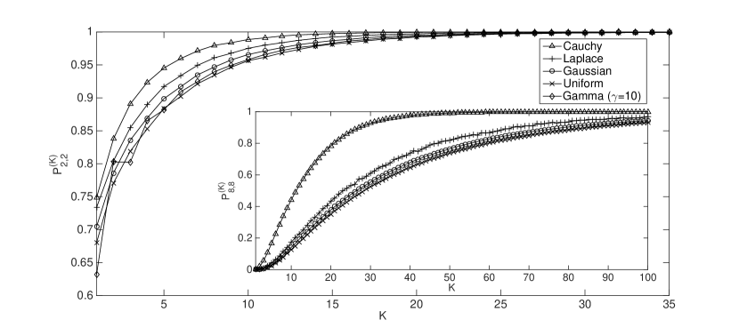
Figure 1: Comparison of probability that all eigenvalues are real for a product of $K$ random matrices with different symmetric distributions and the dimensionality $n=2$ (main) and $8$ (inset). The plot is based on $10^{5}$ independent realizations.

The increase in the probability of all real eigenvalues is reflected in the average number of real eigenvalues as well which is given by $E_{n}^{(K)}=\sum^{n}_{k=0}kP_{n,k}^{(K)}$. Since, as discussed above, the probability $P_{n,k}^{(K)}\to\delta_{n,k}$ as $K$ increases, the average $E_{n}^{(K)}$ approaches the dimension of the matrix. Numerical results in Fig. (3) for $8\times 8$ matrices strongly suggest an exponential approach of the expected number of real eigenvalues to the dimension of the matrix. The data also points to the continuance of the hierarchy even for the average number of real eigenvalues indicating a more microscopic adoption of the hierarchy to all $P^{(K)}_{n,k}$.

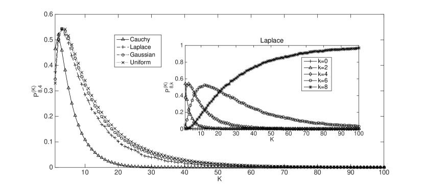
Figure 2: Probability that $4$ eigenvalues are real for a product of $K$ $8\times 8$ random matrices whose elements are chosen from uniform, Gaussian, Laplace and Cauchy distributions, each with zero mean, based on $10^{6}$ realizations. The inset shows the probability that $k$ eigenvalues are real for a product of $K$ $8\times 8$ zero mean, Laplace-distributed random matrices.

III.2 Effect of correlations between matrix elements

III.2.1 Hadamard product

We now consider the Hadamard (or Schur) product wherein the elements of the product are simply the products of the corresponding elements. Thus if $\circ$ is used to denote the Hadamard product of two matrices $A$ and $B$, then $(A\circ B)_{ij}=A_{ij}B_{ij}$. The Hadamard product of two positive semidefinite matrices is also positive semidefinite, unlike the usual product, and is one of the reasons it is important Horn and Johnson (1987). However the reason why we choose to study Hadamard products is that although the matrix elements of the product matrix are products of random numbers, there is no correlation amongst the matrix elements. Thus one can hope to disentangle two possible mechanisms that may be responsible for the phenomenon that all the eigenvalues of a random product matrix tend to be real: the act of simple multiplication which is presumably causing the matrix elements to have large weight near the origin and the various addition of such products that are leading to correlations between the matrix elements.

To this end, we consider the eigenvalue properties of a Hadamard product of $K$ random $n\times n$ matrices with elements distributed according to uniform, Laplace, Gaussian and Cauchy distributions, each with zero mean. Figure (4) shows the case of Hadamard products of $2\times 2$ matrices, and we observe that the hierarchy effect is maintained at any $K$ (although there are more fluctuations in this case as compared to that of the ordinary matrix product). But, importantly, we find that the probability does not approach unity with increasing $K$.

We can get some insight into this result by calculating the distribution of the matrix elements of the Hadamard product matrix for some distributions, and appealing to the results for the $2\times 2$ matrices obtained earlier in Sec. II. Let us first consider the case of Hadamard product of matrices with elements drawn from the bounded distribution $p_{0,\nu}(x)$ defined in Eq. (15). Let $z_{K}=x_{1}x_{2}...x_{K}$ represent a random variable formed by the product of $K$ i.i.d. random variables. As discussed in Appendix E, the distribution of the product for this case is given by

$$\begin{split}p_{K}(z_{K}=x_{1}x_{2}...x_{K})=\frac{(\nu+1)^{K}|z_{K}|^{\nu}}{2(K-1)!}~{}\left[\ln\left(\frac{1}{|z_{K}|}\right)\right]^{K-1}\Theta(1-|z_{K}|).\end{split}$$ (30)

For $\nu\leq 0$, the above distribution diverges at the origin while for positive $\nu$, it vanishes at $|z|=0$ and $1$ and is a nonmonotonic function of $|z|$. Thus, except for the uniform case, the behavior of the distribution $p_{K}(z_{K})$ is similar to that of $p_{0,\nu}$ near the origin. Using the above result, it is possible to numerically evaluate the integral in (5) to obtain $P^{(K)}_{2,2}$ for various values of $\nu$ and $K$. For example, for $\nu=0$, we find the probability of real eigenvalues to be $0.738779$, $0.767331$, $0.782558$, $0.792032$, $0.798561$, $0.803376$ for $K=2,3,4,5,6,7$ respectively. For larger $K$, numerical integration does not converge; however, as shown in Fig. 4 for some representative values of $\nu$, the data obtained from direct sampling indicates the approach to a probability less than $7/8$. For the case of uniform distribution, the probability seems to saturate around $0.84$. But for negative and positive $\nu$, the probability of real eigenvalues approaches a value higher and lower than $0.84$ respectively. This pattern is consistent with the results in Sec. II where the probability of real eigenvalues decreased with increasing $\nu$.

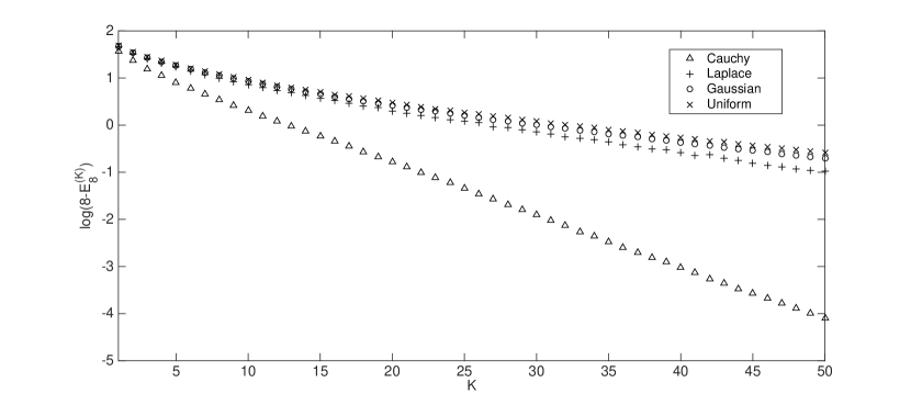
Figure 3: Expected number of real eigenvalues for a product of $K$ random $8\times 8$ matrices with elements chosen from uniform, Gaussian, Laplace and Cauchy distributions, each with zero mean. The plot is based on $10^{6}$ realizations.

We next consider unbounded distributions, and start with the case of Hadamard product of matrices with Gaussian distributed elements with zero mean and unit variance for which Springer and Thompson (1970); Forrester (2014)

$$\begin{split}p_{2}(z_{2})=~{}\frac{1}{2\pi}\int_{-\infty}^{\infty}\int_{-\infty}^{\infty}e^{-x_{1}^{2}/2}e^{-x_{2}^{2}/2}~{}\delta(z_{2}-x_{1}x_{2})~{}dx_{1}dx_{2}\\ =\frac{1}{2\pi}\int_{-\infty}^{\infty}e^{-|z_{2}|\cosh x_{1}}~{}dx_{1}=\frac{K_{0}(|z_{2}|)}{\pi},~{}z_{2}\in(-\infty,\infty).\end{split}$$ (31)

which diverges logarithmically at the origin since $K_{0}(z)\to\ln(1/z)$ as $z$ approaches zero. For this distribution, the integral in Eq. (5) can be numerically evaluated by using the fact that its convolution is given by a Laplace distribution (shown in Sec. III B 2) yielding $P^{(2)}_{2,2}=0.757164$, which is consistent with the value obtained in Fig. (4) by direct sampling. For $K>2$, the probability distributions are given by the Meijer-G functions Springer and Thompson (1970); Forrester (2014) making it difficult to handle this using Eq. (5). We therefore give the results obtained via numerical sampling in Fig. 4 which again indicates an approach towards $0.84$. In the case of Hadamard product of two matrices with Laplace-distributed elements with zero mean given by (24) with $\gamma=1$, we have Springer and Thompson (1970)

$$\begin{split}p_{2}(z_{2})=~{}\frac{1}{4}\int_{-\infty}^{\infty}\int_{-\infty}^{\infty}e^{-|x_{1}|}e^{-|x_{2}|}~{}\delta(z_{2}-x_{1}x_{2})~{}dx_{1}dx_{2}\\ =\frac{1}{2}\int_{-\infty}^{\infty}e^{-2\sqrt{|z_{2}|}\cosh x_{1}}~{}dx_{1}=K_{0}(2\sqrt{|z_{2}|}),~{}z_{2}\in(-\infty,\infty),\end{split}$$ (32)

where the last step in Eq. (32) has been done by a series of two transformations, $x_{1}\rightarrow x_{1}\sqrt{|z_{2}|}$ followed by $x_{1}\rightarrow e^{x_{1}}$. Numerical evaluation of Eq. (5) using this yields $P^{(2)}_{2,2}=0.773849$, and the results obtained from direct sampling show a convergence towards a value close to $0.84$. For the Cauchy-distributed matrix elements, the distribution of the product of two random variables is known to be Springer and Thompson (1966)

$$p_{2}(z_{2})=\frac{\ln z_{2}^{2}}{\pi^{2}(z_{2}^{2}-1)},$$ (33)

which diverges at the origin logarithmically.

Thus, as Fig. (4) shows, the probability of all real eigenvalues monotonically increases with $K$ and saturates to a value in the range $0.82-0.84$. Note that these numbers are less than $7/8$ which, from our analysis in the previous section, is expected of distributions that diverge as a power law, $|x|^{\nu}$ with $\nu\rightarrow-1$, at the origin. From the above calculations for $K=2$, it is clear that the uniform distribution and the three unbounded distributions discussed above have Hadamard product elements distributed according to a probability distribution that diverges as $\ln(1/|x|)$ at the origin. In fact, the elements of the Hadamard product of uniform distribution as well as Cauchy distributed random matrices have probability distributions that diverge as $\ln(1/|x|)^{K-1}$ at arbitrary $K$ Springer and Thompson (1966). It is reasonable to expect that the Gaussian and Laplace cases also diverge in a similar manner. For these cases, as the divergence at the origin is somewhat “slower” than a power law, it seems reasonable that the probability of eigenvalues being real is a shade smaller than that of single $2\times 2$ matrices whose elements are distributed according to the power law discussed above.

Assuming that the probability of Hadamard products saturate to the same value for these four distributions in the $K\rightarrow\infty$ limit, and taking this to be $\approx 0.846$ (in the case of $n=2$), our numerical results show a power law approach to the constant:

$$P^{(K)}_{2,2}=P^{(\infty)}_{2,2}-\dfrac{C}{K^{\theta}},$$ (34)

where $C$ is a positive constant and the exponent $\theta\approx 0.675,0.649,0.654,0.621$ for uniform, Gaussian, Laplace and Cauchy distribution respectively (see the inset of Fig. (4)). Thus, here the probability of real eigenvalues approaches the asymptotic value as a power law in comparison to the ordinary matrix product case, where this approach is seen to be exponentially fast Lakshminarayan (2013). The exponential behavior is also seen in the expected values of real eigenvalues as in Fig. 3. We also looked at the fraction of expected number of real eigenvalues for higher dimensional matrices ($n=2,3,4$) when each matrix in the Hadamard product has Gaussian-distributed elements with zero mean, and find that the fraction of real eigenvalues increases and saturates to a value less than one, unlike that observed for the case of usual matrix products. We also find that the asymptotic value of this fraction decreases with an increase in the dimensionality of the matrices.

The convergence of the probability that all eigenvalues are real as $K\to\infty$ for the Hadamard product can also be understood using the Central Limit Theorem applied to the logarithm of the absolute value of the product random variable. The elements of the Hadamard product matrix would then admit a symmetrized log-normal probability distribution of the form Sornette (2000)

$$\begin{split}p_{K}(z_{K}=x_{1}x_{2}...x_{K})=\frac{1}{2|z_{K}|\sqrt{2\pi K\sigma^{2}}}~{}\exp\left[-\frac{(\log|z_{K}|-K\mu)^{2}}{2K\sigma^{2}}\right],~{}z_{K}\in(-\infty,\infty),\end{split}$$ (35)

for large $K$, with the parameters $\mu$ and $\sigma$ being the mean and standard deviation of $\log|x|$. Numerically, we find that the probability that all eigenvalues are real for a matrix with elements distributed according to Eq. (35) indeed converges to a value around $0.84$ at large $K$, as for the Hadamard product.

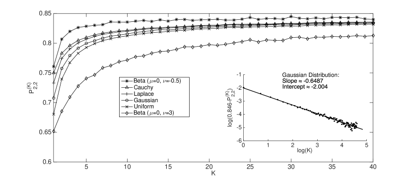
Figure 4: Comparison of probability that all eigenvalues are real for Hadamard products of $K$ $2\times 2$ random matrices for some symmetric distributions based on $10^{5}$ realizations. For the Beta distribution with $\nu=3$, the x-axis is scaled up by a factor $5$ since the convergence to the asymptotic value occurs for very large $K$. The inset shows the power law approach of the probability of all real eigenvalues to the asymptotic value which is less than unity, for the Gaussian case. The plot is based on $10^{5}$ realizations for the Beta distribution, and $10^{6}$ for the rest.

III.2.2 Usual matrix product

We now return to the properties of the matrix obtained after multiplying $K$ matrices, and ask why the asymptotic probability of real eigenvalues saturates to unity unlike that for the Hadamard product. We can think of two possible reasons: one, the (usual) product matrix elements have probability distributions that are significantly different from the Hadamard case. The other possibility is that the correlations between the matrix elements in the case of usual products lead to an increase in probability of all eigenvalues real to unity as opposed to the Hadamard case where this is not true. It is not obvious whether the difference in the probability distribution or the correlations between the matrix elements is responsible for a higher $P^{(K)}_{2,2}$.

To gain some insight into this intriguing question, we looked at the matrices with i.i.d. random variables as elements, each distributed according to the probability distribution of the product matrix elements at various $K$. Such matrices can be easily generated by taking independent samples of usual product matrices at each $K$ and forming new matrices by picking the corresponding matrix elements from the independent product matrix samples. These new matrices would then have elements with probability distributions corresponding to that of elements of a usual product matrix at product length $K$, but the matrix elements would now be independent, having been selected from independent product matrix samples. Fig. (5) shows a comparison between $P^{(K)}_{2,2}$ for the Hadamard product and usual product and $P^{(1)}_{2,2}$ for matrices with probability distribution of elements corresponding to that of usual product at product length $K$, but without any correlations between the elements. It is clear that the difference in probability distribution of matrix elements between the Hadamard and the usual product has an effect of lowering $P^{(K)}_{2,2}$ for the usual product case to a value below that of the Hadamard product case. However, the presence of correlations between the matrix elements of the usual product matrix is seen to have an effect of a substantial increase in $P^{(K)}_{2,2}$, finally leading to an asymptotic value of one.

The effect of correlations can be seen analytically for the case of Gaussian-distributed matrices when $K=2$. We have seen that the distribution of the product of two Gaussian-distributed random variables with zero mean and unit variance is given by Eq. (31) and the probability of real eigenvalues is $0.757164$. The distribution of the matrix elements obtained on taking the usual matrix product corresponds to that of the sum of two random variables, each distributed according to the distribution of the product of two random variables. The characteristic function of Eq. (31) is given by ${\tilde{p}}(k)=(1+k^{2})^{-1/2},~{}k\in[-1,1]$ (due to Eq. (11.4.14) of Abramowitz and Stegun (1964)). It is easily seen that this ${\tilde{p}}(k)$ is the square root of the characteristic function of Laplace distribution. Hence, the product matrix elements have a Laplace distribution, for which we know from Eq. (56) that $P^{(1)}_{2,2}$ would have been $11/15=0.7333$, had the elements been independent. But, the correlations between the matrix elements raise this probability to $\pi/4=0.7854$ Lakshminarayan (2013); Forrester (2014) for the usual product, hence presenting a strong evidence that the correlations between the matrix elements are in fact leading to $P^{(K)}_{2,2}\rightarrow 1$ observed for usual products.

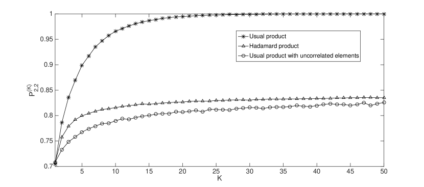
Figure 5: Comparison of $P^{(K)}_{2,2}$ for Hadamard products and usual products with correlated elements and $P^{(1)}_{2,2}$ for matrices with i.i.d elements distributed according to probability distribution of product of $K$ independent matrices, for $2\times 2$ zero mean, Gaussian-distributed random matrices. The plot is based on $10^{6}$ realizations for the Hadamard product, and $10^{5}$ for the rest.

We also measured the correlations between the matrix elements to see how correlations increase with increasing $K$ for $2\times 2$ matrices with Gaussian-distributed matrix elements. More precisely, we consider

$$C_{i}=\left(\frac{\langle x_{1}x_{i}\rangle-\langle x_{1}\rangle\langle x_{i}\rangle}{K}\right)^{1/K}~{},~{}i=1,...4$$ (36)

where $x_{i}$ are the matrix elements obtained after taking the product of $K$ matrices. For $K=1$, obviously $C_{i}=\delta_{i,1}$. But with increasing $K$, all the four $C_{i}$’s seem to be of same order i.e. the variance of the new distribution and the correlations are similar. In particular, we find that for $K=2$, the correlations $C_{i}=1.417,0.047,0.031,0.057$ for $i=1,2,3,4$ respectively, but these numbers increase to $1.885,1.446,1.349,1.462$ and $1.905,1.500,1.475,1.667$ for $K=12$ and $20$ respectively. These data suggest that similar to the probability $P_{2,2}^{(K)}$, the correlations also tend to saturate with increasing $K$.

IV Discussion

How does the probability of real eigenvalues for a $2\times 2$ random matrix depend on the probability distribution of the matrix? It is quite surprising that such an apparently elementary question presents many novel challenges, and throws up some surprises. Here we find that the probability of real eigenvalues depends on several detailed features of the probability distribution, some of which we have identified here as the finiteness and smoothness at the origin, existence of maxima away from origin and the finitness of the moments. We have shown that eigenvalues are most likely to be real for distributions limiting to $p(x)\sim 1/|x|$ which is the most divergent distribution at the origin (with zero mean) and occur with a probability $7/8=0.875$. That the large weight at the origin correspond to high probability is perhaps not surprising since when the matrix elements are distributed according to $\delta(x)$, this probability is unity. However, interestingly, here we find the maximum probability to be less than one. The origin of this naturally rests in the smoothness of the probability distributions considered. We also mention that the values are not universal; for example, the probability turns out to be different for the Beta distribution $p_{0,2}(x)$ and for Gamma distributed matrix elements with $\gamma=3$, although both have the same behavior near $x=0$.

Our results suggest that the probability that all eigenvalues are real is larger for distributions with large weight at the origin and that decay slowly. More concretely, there exists a hierarchy between the probability values of the different distributions, which is Cauchy (0.750) $>$ Laplace (0.733) $>$ Gaussian (0.707) $>$ uniform (0.6805). Moreover, for class of distributions that decay in the same manner, the distributions with higher weight close to zero have a higher probability of real eigenvalues. For example, although the probability $p_{2,2}^{(1)}$ for distribution Eq. (24) for $\gamma\leq 2$ is larger than the uniform distribution as it decays slower than the bounded distribution, this probability for $n=3$ is found to be smaller than that for the uniform case. Thus the ‘reality’ is determined by both the tail and near-zero behavior of the probability distribution from which the matrix elements have been chosen. For the broad class of smooth distributions we have considered, we did not find the probability of real eigenvalues to lie outside the range $[5/8,7/8]$, which appear to be natural boundaries for sufficiently smooth distributions.

Numerical results discussed above also shows that this remains valid even after taking a product of random matrices. It is quite surprising that the curves for probabilities of the different distributions do not cross each other. An intuitive explanation of this is yet to be figured out. We also measured the distribution of the matrix elements of the product matrix, and find that it decays slower (but faster than any power law) as the number $K$ in the product increases. This observation is consistent with the result for single matrices (with finite moments), namely, that faster the distribution decays, smaller is the probability that all eigenvalues are real. However this is only part of the explanation as the probability $p_{N,N}^{(K)}$ always stays below unity when correlations between matrix elements are ignored, and in order to approach unity, correlations are found to be crucial. It maybe stated that despite extensive and exact results obtained so far there is not much understanding about why the eigenvalues tend to become real under the usual matrix product, and more work in this direction is clearly desired.

Appendix A Detailed derivations for symmetric beta distribution

When $\mu=0$ and $\nu=2k$ is a positive integer, the convolution can be written in the form of a finite series:

$$q(z)=\Theta(2-|z|)\left(\frac{2k+1}{2}\right)^{2}\sum_{r=0}^{2k}\binom{2k}{r}(-|z|)^{2k-r}\dfrac{1-(|z|-1)^{2k+r+1}}{2k+r+1}.$$ (37)

Integrations can be done using the hyperbolic variables as the combination $xy$ appears exclusively. To outline the method used, hyperbolic coordinates ($v,w$) where $x=ve^{w}$ and $y=ve^{-w}$ are useful. Thus the variable $w$ does not appear in the transformed expression. The range of $v$ is $[0,1]$, while for a given $v$, the range of $w$ is $[\ln v,-\ln v]$. The integration over $w$ is easily carried out first, and noting that the Jacobian of the transformation is $2v$, leads finally to:

$$\begin{split}P^{(1)}_{2,2}(\mu=0,\nu=2k)=1-(2k+1)^{4}\times\sum_{r=0}^{2k}\left[\binom{2k}{r}\dfrac{2^{2k-r+1}}{2k+r+1}\left(\dfrac{(-1)^{r}}{(2k-r+1)(6k-r+3)^{2}}\right.\right.+\\ \left.\left.\sum_{l=0}^{2k+r+1}\binom{2k+r+1}{l}\dfrac{(-2)^{l}}{(2k-r+l+1)(6k-r+l+3)^{2}}\right)\right].\end{split}$$ (38)

As special cases:

$$P^{(1)}_{2,2}(\mu=0,\nu=2)=\dfrac{8905}{14112}=0.631023,\;P^{(1)}_{2,2}(\mu=0,\nu=4)=\dfrac{45332489}{72144072}\approx 0.628361.$$ (39)

The case of odd integer $\nu$ is also accessible, however we only state the result when $\nu=1$. The convolution is now piecewise continuous on $|z|<1$ and $1<|z|<2$, and the probability of real eigenvalues is

$$P_{2,2}^{(1)}(\mu=0,\nu=1)=\frac{3653}{5760}+\frac{\ln 2}{240}\approx 0.63709.$$ (40)

To understand the behavior of the probability of real eigenvalues for negative $\nu$, it is convenient to write the convolution for the distribution $p_{0,\nu}(x)$ defined by Eq. (15) as

$$\begin{split}&q(z)=\int_{-\infty}^{+\infty}p(x)p(z-x)\,dx\\ &=\left(\frac{\nu+1}{2}\right)^{2}\int_{-1}^{+1}|x|^{\nu}|z-x|^{\nu}\Theta(1-|z-x|)\,dx.\end{split}$$ (41)

Note that $|x|\leq 1$ and $|z-x|\leq 1$ implies that $|z|\leq 2$. From the symmetry $q(z)=q(-z)$ it suffices to consider $0\leq z\leq 2$. Using the hyperbolic coordinates, $x=ve^{w}$ and $y=ve^{-w}$, we get

$$\begin{split}&P_{2,2}^{(1)}=1-(\nu+1)^{2}\int_{0}^{1}2v\,dvv^{2\nu}\int_{\ln v}^{-\ln v}dw\int_{0}^{2v}dzq(z)\\ &=1+(1+\nu)^{4}\int_{0}^{1}v^{1+2\nu}\ln v\int_{0}^{2v}dz\,\int_{-1}^{1}|x|^{\nu}|x-z|^{\nu}\Theta(1-|x-z|)dx\,dv.\end{split}$$ (42)

Except when $\nu$ is an even integer, some care must be taken as $q(z)$ is piecewise continuous in the two intervals $[0,1]$ and $[1,2]$. For $\nu=-1/2$, we have

$$P_{2,2}^{(1)}(\mu=0,\nu=-1/2)=\frac{1}{48}(41-\pi-2\ln 2)\approx 0.759836.$$ (43)

To find the probability as $\nu\to-1$, consider the two inner integrals over $z$ and $x$ in Eq. (42). On considering various cases arising due to the Heaviside theta function and performing the integral over $z$ first, we get

$$P_{2,2}^{(1)}(\mu=0,\nu)=\frac{3}{4}-\frac{\Gamma(\frac{1}{2})\Gamma(2+\nu)}{\Gamma(\frac{3}{2}+\nu)}~{}\frac{1+4(1+\nu)\ln 2}{4^{2(2+\nu)}}-J_{1}+J_{2},$$ (44)

where

$$J_{1}=(1+\nu)^{2}\left(\int_{0}^{1/2}dv~{}v^{1+2\nu}\ln v~{}(1-2v)^{1+\nu}-\int_{1/2}^{1}dv~{}v^{1+2\nu}\ln v~{}(2v-1)^{1+\nu}\right),$$ (45)

and

$$J_{2}=(1+\nu)^{3}\left(2\int_{0}^{1/2}dv~{}v^{2+2\nu}\ln v\int_{0}^{1-2v}dx~{}(x(2v+x))^{\nu}+\int_{1/2}^{1}dv~{}v^{1+2\nu}\ln v\int_{2v-1}^{1}dx~{}x^{\nu}(2v-x)^{1+\nu}\right).$$ (46)

It is clear that when $\nu\to-1$, the second term on the right hand side of both $J_{1}$ and $J_{2}$ is zero. The first integral in $J_{1}$ contributes $-1/4$ when the integral is carried out by expanding the integrand around $v=0$. However, the dominant contribution to the first integral in $J_{2}$ comes when both $x$ and $v$ are small. Then it is useful to split the integral over $v$ from $0$ to $1/4$ and $1/4$ to $1/2$ and it turns out that the former integral with $x$ lying in the range $0$ to $2v$ contributes $-1/16$ to $J_{2}$. Using these results and setting $\nu=-1$ in the second term in Eq. (44), we finally obtain the desired result, viz., $P_{2,2}^{(1)}(\mu=0,\nu\to-1)=7/8$.

Appendix B Detailed derivations for smooth bounded distributions

For the case $\eta=1$ (parabolic distribution), the convolution is still calculable as:

$$q(z)=\frac{3}{160}(2-|z|)^{3}(4+6|z|+z^{2})\Theta(2-|z|).$$ (47)

The integrals in Eq. (5) are then elementary and are easily done with mathematical packages, and yield the probability

$$P_{2,2}^{(1)}(\eta=1)=\dfrac{489341}{705600}=0.69351.$$ (48)

The case for $\eta=2$ leads to longer expressions, but with Mathematica, it is easy to evaluate the convolution and the resultant probability as

$$q(z)=\dfrac{5}{14}\dfrac{1}{16^{2}}(2-|z|)^{5}(16+40|z|+36z^{2}+10|z|^{3}+z^{4})\Theta(2-|z|),$$ (49)

and

$$P_{2,2}^{(1)}(\eta=2)=\dfrac{180521487191}{258564354048}\approx 0.698168.$$ (50)

Similar analysis yields the probability for $\eta=5,10,20,50$ as $0.702769,0.704785,0.705906,0.706616$ respectively. A monotonic convergence of the probability to $1/\sqrt{2}$ as $\eta$ increases is then a reasonable indication from these calculations.

Appendix C Detailed derivations for Gaussian distribution

For the Gaussian distribution (23), the convolution with itself is also a Gaussian distribution but with variance of $2$ rather than $1$: $q(z)=e^{-z^{2}/4}/(2\sqrt{\pi})$. Application of Eq. (5), along with the usage of hyperbolic coordinates results in

$$P^{(1)}_{2,2} = 1-\frac{1}{\pi^{3/2}}\int_{0}^{\infty}e^{(x^{2}+y^{2})/2}\int_{0}^{2\sqrt{xy}}e^{-z^{2}/4}dz\;dx\,dy$$ (51)

$$= 1-\frac{1}{\pi^{3/2}}\int_{0}^{\infty}2vdv\int_{-\infty}^{\infty}e^{-v^{2}\cosh 2w}dw\int_{0}^{2v}e^{-z^{2}/4}dz.$$ (52)

The integral over $v$ becomes elementary when the burden of a finite range of integration is shifted from the $z$ variable to the variable $v^{2}$. That is, the $v$ integral is done first following writing the $z$ integral as $e^{-z^{2}/4}\Theta(-z+2v)$ over the interval $[0,\infty)$. The probability of real eigenvalues simplifies to

$$P^{(1)}_{2,2}=1-\frac{2}{\pi\sqrt{2}}\int_{0}^{\infty}\dfrac{dw}{\cosh 2w\cosh w}=\dfrac{1}{\sqrt{2}}.$$ (53)

This follows as the integral can be evaluated as $\pi(\sqrt{2}-1)/2$ either with packages such as Mathematica, or with the use of the residue theorem. This is applied to a rectangular contour with base on the interval $[-L,L]$, and the top on the interval with $\mbox{Im}(w)=i\pi$ and $\mbox{Re}(w)\in[-L,L]$. This region encloses three poles of order $1$ at $i\pi/4,\,i\pi/2$ and $i3\pi/4$. In the limit of large $L$, the contour integral is twice what is required.

If we follow the path of the characteristic function, we have ${\tilde{p}}(\omega)=e^{-\omega^{2}}.$ Computing the integral in Eq. (9) yields:

$$P_{2,2}^{(1)}=1-\frac{2}{\pi\sqrt{\pi}}\sum^{\infty}_{n=0}\frac{(-1)^{n}}{n!(2n+1)}2^{n-\frac{1}{2}}\left[\Gamma\left(\frac{n}{2}+\frac{3}{4}\right)\right]^{2}.$$ (54)

A numerical approximation to Eq. (54) using Mathematica yields a value which is exactly equal to $1/\sqrt{2}$. Also, using the properties of Gamma functions, it is possible to modify this series to obtain

$$P_{2,2}^{(1)}=1-\frac{1}{2\pi}\sum^{\infty}_{n=0}\frac{(-1)^{n}}{n!}\frac{\Gamma\left(n+\frac{1}{2}\right)\Gamma\left(\frac{n}{2}+\frac{3}{4}\right)}{\Gamma\left(\frac{n}{2}+\frac{5}{4}\right)},$$

which has already been shown to be exactly equal to $1/\sqrt{2}$ in Lakshminarayan (2013).

Appendix D Detailed derivations for Gamma distribution

For $\gamma=1$, we have the so-called Laplace distribution $p(x)=(1/2)e^{-|x|}$ for which $p_{\gamma}(0)$ is nonzero. Using the linear transformation formula (15.3.3) of Abramowitz and Stegun (1964) and the definition of the Gauss hypergeometric function ${{}_{2}}F_{1}(a,b;c;z)$ in Eq. (9), after some algebra, we obtain

$$P_{2,2}^{(1)}(\gamma=1) = 1-\frac{1}{2}\int^{\infty}_{0}d\omega(1+\omega^{2})^{-7/2}$$ (55)

$$= \frac{11}{15}\approx 0.733333.$$ (56)

For integer $\gamma$, similar steps can be used to find an analytical expression for $P_{2,2}^{(1)}$.

The convolution is given by

$$q(z)=\dfrac{1}{4\Gamma(\gamma)^{2}}\int_{-\infty}^{\infty}|x-z|^{\gamma-1}|x|^{\gamma-1}e^{-|x|}e^{-|x-z|}dx.$$ (57)

Note that the general symmetry $q(z)=q(-z)$ holds, and we can therefore restrict attention to $z\geq 0$. This simplifies the computation somewhat and leads to Thus the convolution is itself the sum of a Gamma distribution and a Bessel distribution McKay (1932). If the distribution was not symmetrized, that is the distribution were the usual Gamma distribution on $[0,\infty)$, only a term proportional to the first will be in the convolution. The second term represents the convolution of the distributions on the opposite sides of the maxima. Now to evaluate the probability of real eigenvalues of a $2\times 2$ matrix with entries from the symmetric Gamma distribution, we use the first equality in Eq. (5), and obtain

$$P_{2,2}^{(1)}(\gamma)=\dfrac{1}{2}+\frac{1}{\Gamma(\gamma)^{2}}\int_{0}^{\infty}dx\int_{0}^{\infty}dy\,(xy)^{\gamma-1}e^{-x-y}\int_{2\sqrt{xy}}^{\infty}dz\,q(z).$$ (58)

Once again, using the hyperbolic coordinates, $x=ve^{w}/2,y=ve^{-w}/2$ and performing the integral over $w$ results in

$$P_{2,2}^{(1)}(\gamma)=\dfrac{1}{2}+\frac{1}{2^{2\gamma-2}\Gamma(\gamma)^{2}}\int_{0}^{\infty}dv\,v^{2\gamma-1}K_{0}(v)\int_{v}^{\infty}dz\,q(z).$$ (59)

We first consider the parameter regime $\gamma<1$. Apart from $\gamma=1$ the other “easy” case is $\gamma=1/2$ where we find

$$P_{2,2}^{(1)}(\gamma=1/2)=\frac{1}{2\pi}+\frac{5}{8}\approx 0.784155.$$ (60)

In fact, evaluation of such integrals with packages like Mathematica, even in this case, return unevaluated hypergeometric functions. However, in this case, one can simplify the integrals directly (hypergeometric functions encountered do not seem to have known identities, at least to our knowledge). For instance, in the evaluation with the Bessel distribution part of the convolution, one needs

$$\frac{1}{\pi^{2}}\int_{0}^{\infty}\int_{0}^{\infty}K_{0}(v)K_{0}(v+z)\,dv\,dz=\dfrac{1}{2\pi^{2}}\int_{0}^{\infty}\dfrac{u\,du}{\sinh u}=\dfrac{1}{8},$$ (61)

which is obtained by using the integral representation of the Bessel function of zeroth order and simplifying. The integral with the first term of $q(z)$ is more easily evaluated to $1/(2\pi)$. Thus the probability is $1/2+1/(2\pi)+1/8$ as stated above. Numerical evaluation of these integrals is also tricky as $\gamma$ decreases toward zero.

For $\gamma>1$, the distribution $P_{2,2}^{(1)}(\gamma)=(1/2)+A_{1}(\gamma)+A_{2}(\gamma)$ where

$$A_{1}(\gamma)=\dfrac{\sqrt{\pi}}{2^{4\gamma}\Gamma(\gamma)^{2}}\sum_{k=0}^{2\gamma-1}\frac{1}{2^{k}k!}\dfrac{\Gamma(k+2\gamma)^{2}}{\Gamma(k+2\gamma+\frac{1}{2})},\;\;A_{2}(\gamma)=\dfrac{\Gamma(\gamma+\frac{1}{2})^{2}}{4\sqrt{\pi}\Gamma(\gamma)^{2}}\sum_{k=0}^{\gamma-1}\frac{1}{k!}\dfrac{\Gamma(k+\gamma)^{2}}{\Gamma(k+2\gamma+\frac{1}{2})}.$$ (62)

The sums above maybe written in terms of hypergeometric functions, but they do not appear to be simple expressions. To state some other exact values for the probability of real eigenvalues:

$$P^{(1)}_{2,2}(2)=\dfrac{10259}{15015},\,\,P^{(1)}_{2,2}(3)=\dfrac{640561}{969969}.$$ (63)

The sum $A_{1}(\gamma)$ for large $\gamma$ can be approximated by

$$A_{1}(\gamma)\approx\frac{\sqrt{\pi}\gamma^{2}}{2^{4\gamma}(\gamma!)^{2}}~{}\sum_{k=0}^{2\gamma}\frac{1}{2^{\gamma}}~{}\frac{1}{(2\gamma+k)^{3/2}}~{}\frac{(2\gamma+k)!}{k!},$$ (64)

where we have used that the ratio $x!/(x+\frac{1}{2})!\approx x^{-1/2}$ for large $x$. Employing the Stirling’s approximation $s!\approx\sqrt{2\pi s}(s/e)^{s}$ in the above equation, and replacing the sum by an integral, we obtain

$$A_{1}(\gamma)\approx\frac{1}{4\sqrt{\pi}}\int_{0}^{2\gamma}\frac{dk}{\sqrt{k}}~{}\frac{2\gamma}{2\gamma+k}\exp\left[2\gamma~{}g\left(\frac{k}{2\gamma}\right)\right],$$ (65)

where

$$g(x)=\ln(1+x)+x\ln(1+x^{-1})-(1+x)\ln 2.$$ (66)

On evaluating the integral in Eq. (65) by saddle point method, we obtain $A_{1}(\gamma)=(1/8)\textrm{erf}(\sqrt{\gamma/2})$ which, for large $\gamma$, gives $1/8$. An analysis similar to above also shows the leading order correction in $A_{1}(\gamma)$ to be $(16\sqrt{2\pi\gamma})^{-1}$, and $A_{2}(\gamma)$ to be exponentially small in $\gamma$.

Appendix E Distribution of the product for the probability distribution Eq. (15)

For the distribution $p_{0,\nu}(x)$ defined by Eq. (15), the distribution of the product is given by

$$p_{K}(z_{K}) = \left(\frac{1+\nu}{2}\right)^{K}\int_{-1}^{1}dx_{1}...\int_{-1}^{1}dx_{K}~{}|x_{1}|^{\nu}...|x_{K}|^{\nu}~{}\delta(z_{K}-\prod_{i=1}^{K}x_{i})$$ (67)

$$= \frac{1}{2}~{}(1+\nu)^{K}~{}\int_{0}^{1}dx_{1}...\int_{0}^{1}dx_{K}~{}x_{1}^{\nu}...x_{K}^{\nu}~{}\delta(|z_{K}|-\prod_{i=1}^{K}x_{i}),$$ (68)

where the last equation follows on noting that one half of the $2^{K}$ cases corresponding to the sign of the set $\{x_{i}\}$ contribute equally to positive $z_{K}$. On carrying out the integral over $x_{K}$, we have

$$p_{K}(z_{K}) = \frac{1}{2}~{}(\nu+1)^{K}~{}|z_{K}|^{\nu}\int_{|z_{K}|}^{1}\frac{dx_{1}}{x_{1}}\int_{\frac{|z_{K}|}{x_{1}...x_{K-3}}}^{1}\frac{dx_{2}}{x_{2}}...\int_{\frac{|z_{K}|}{x_{1}...x_{K-2}}}^{1}\frac{dx_{K-1}}{x_{K-1}}$$ (69)

$$= \frac{1}{2}~{}\frac{(\nu+1)^{K}}{(K-1)!}~{}|z_{K}|^{\nu}~{}\left[\ln\left(\frac{1}{|z_{K}|}\right)\right]^{K-1}~{},~{}|z_{K}|<1.$$ (70)

The above result can be obtained by either transforming the problem of the distribution of product to that of sum by writing $\ln x_{i}=y_{i}$, or directly using Mellin transforms Springer and Thompson (1966).

References

- Littlewood and Offord (1939) J. E. Littlewood and A. C. Offord, Proc. Cambridge Philos. Soc. 35, 133 (1939).
- Edelman and Kostlan (1995) A. Edelman and E. Kostlan, Bull. American Math. Soc. 32, 1 (1995).
- Nguyen et al. (2014) H. Nguyen, O. Nguyen, and V. Vu, arXiv:1402.4628v1 (2014).
- Kac (1943) M. Kac, Bull. American Math. Soc. 49, 314 (1943).
- Stevens (1969) D. C. Stevens, Comm. Pure Appl. Math. 22, 457 (1969).
- Logan and Shepp (1966) B. F. Logan and L. A. Shepp, Proc. London Math. Soc. 18, 29 (1966).
- Edelman et al. (1994) A. Edelman, E. Kostlan, and M. Shub, J. Amer. Math. Soc. 7, 247 (1994).
- Edelman (1997) A. Edelman, J. Multivariate Anal. 60, 203 (1997).
- Kanzieper and Akemann (2005) E. Kanzieper and G. Akemann, Phys. Rev. Lett. 95, 230201 (2005).
- Furstenberg and Kesten (1960) H. Furstenberg and H. Kesten, Annals of Mathematics Statistics 31, 457 (1960).
- Bougerol and Lacroix (1985) P. Bougerol and J. Lacroix, Products of random matrices with applications to Schrödinger operators (Birkhauser, Boston-Basel-Stuttgart, 1985).
- Crisanti et al. (1993) A. Crisanti, G. Paladin, and A. Vulpiani, Products of Random Matrices in Statsitical Physics (Springer-Verlag, Berlin-Heidelberg, 1993).
- Roga et al. (2011) W. Roga, M. Smaczynski, and K. Zyczkowski, Acta Phys. Pol. B 42, 1123 (2011).
- Burda et al. (2012) Z. Burda, M. A. Nowak, and A. Swiech, Phys. Rev. E 86, 061137 (2012).
- Akemann and Ipsen (2015) G. Akemann and J. R. Ipsen, arXiv:1502.01667v2 (2015).
- Shuddhodan et al. (2011) K. V. Shuddhodan, M. S. Ramkarthik, and A. Lakshminarayan, J. Phys. A 44, 345301 (2011).
- Lakshminarayan (2013) A. Lakshminarayan, J. Phys. A 46, 152003 (2013).
- Forrester (2014) P. J. Forrester, J. Phys. A 47, 065202 (2014).
- Ipsen (2015) J. Ipsen, J. Phys. A 4, 155204 (2015).
- Beenakker et al. (2013) C. W. J. Beenakker, J. M. Edge, J. P. Dahlhaus, D. I. Pikulin, S. Mi, and M. Wimmer, Phys. Rev. Lett. 111, 037001 (2013).
- Contopoulos et al. (1994) G. Contopoulos, S. C. Farantos, H. Papadaki, and C. Polymilis, Phys. Rev. E 50, 4399 (1994).
- (22) DLMF, NIST Digital Library of Mathematical Functions, http://dlmf.nist.gov/, Release 1.0.9 of 2014-08-29, online companion to Olver:2010:NHMF, URL http://dlmf.nist.gov/.
- Abramowitz and Stegun (1964) M. Abramowitz and I. A. Stegun, Handbook of Mathematical Functions with Formulas, Graphs, and Mathematical Tables (Dover, 1964).
- Horn and Johnson (1987) R. A. Horn and C. R. Johnson, Matrix Analysis (Cambridge University Press, Cambridge, 1987).
- Springer and Thompson (1970) M. D. Springer and W. E. Thompson, SIAM J. Appl. Math 18, 721 (1970).
- Springer and Thompson (1966) M. D. Springer and W. E. Thompson, SIAM J. Appl. Math 14, 511 (1966).
- Sornette (2000) D. Sornette, Critical Phenomena in Natural Sciences (Springer, Berlin, 2000).
- McKay (1932) A. T. McKay, Biometrika 24, 39 (1932).