Configuration Interaction with Antisymmetrized Geminal Powers

Abstract

To avoid the combinatorial computational cost of configuration interaction (CI), we have previously introduced the symmetric tensor decomposition CI (STD-CI) method, where we take advantage of the antisymmetric nature of the electronic wave function and express the CI coefficients compactly as a series of Kronecker product states (STD series) [W. Uemura and O. Sugino, Phys. Rev. Lett. 109, 253001 (2012)]. Here we extend the variational degrees of freedom by using different molecular orbitals for different terms in the STD series. This scheme is equivalent to the linear combination of the Hartree-Fock-Bogoliubov state or the antisymmetrized geminal powers (AGP). The total energy converges very rapidly within 0.72 $\mu$Hartree taking only 10 terms for the water molecule, and the convergence is likewise fast for Hubbard tetramers. The computational cost scales as the fifth power of the number of electrons and the square of the number of terms in the STD series, indicating the promise of this AGP-based scheme for highly accurate and efficient computation of quantum systems.

I Introduction

Determining the ground state of a many-body system is the most basic problem in many fields of science, such as condensed matter physics, nuclear physics and quantum chemistry. Many numerical approaches have been developed so far to obtain the wavefunction. In the configuration interaction (CI)shavitt , multiple quasiparticle states are generated from a mean-field wavefunction and the coefficients for their linear combination are determined by solving an eigenvalue problem, while in the variational Monte Carlo (VMC)foulkes , the quasiparticles are generated stochastically to obtain the expectation value of the total energy to be variationally determined. In the tensor network (TN) frameworkspringer , the total energy is variationally determined using specific quasiparticle states generated according to an assumed TN. In those popular schemes, accessible degrees of freedom are usually not very large. This is particularly the case for CI albeit being the most versatile in that CI is free from the well-known negative sign problem of QMC and the dimensional restriction of the tensor networkspringer . In this view, extending the degrees of freedom accessible by CI is a very important problem.

In the field of quantum chemistry, the CI wavefunction of an $N$-electron system is expanded as

$$\Psi\left(x_{1}\cdots x_{N}\right)=\sum_{i_{1}\cdots i_{N}=1}^{M}A_{i_{1}\cdots i_{N}}\psi_{i_{1}}\left(x_{1}\right)\cdots\psi_{i_{N}}\left(x_{N}\right),$$ (1)

in terms of the molecular orbitals (MOs) $\psi_{i}\left(x\right)$, which are represented as a linear combination of the atomic orbitals (AOs) $\phi_{a}$, as

$$\psi_{i}\left(x\right)=\sum_{a=1}^{M}U_{ia}\phi_{a}\left(x\right),$$ (2)

using elements of an orthogonal matrix $U$. The CI coefficients $A_{i_{1}\cdots i_{N}}$, which are elements of an antisymmetric tensor of order $N$rank and dimension $M$, are varied to minimize the total energy and thus the full-CI calculation is, in practice, hampered by the degrees of freedom that grow combinatorially with $N$. Usually, the CI series is truncated to make the computation tractable; however, when starting from the Hartree-Fock (HF) wavefunction by taking the permutation tensor $\epsilon_{i_{1}\cdots i_{N}}$ in place of $A_{i_{1}\cdots i_{N}}$ and the Hartree-Fock (HF) orbital $\psi_{i}^{HF}$ in place of $\psi_{i}$, the CI series usually converges very slowlyshavitt . The convergence does not, in general, speed up drastically even when starting from multiple Slater determinants. Instead, use of localized MOs in place of the canonical HF orbitals is known to be effective for this purposeLMO , and, recently, significant speed-up was achieved by using non-orthonormal Slater determinants comprised of non-orthonormal MOs that augment the HF orbitalsGoto . It is therefore expected that CI can be made more practicable by using optimal MOs for this purpose.

Apart from CI, the many-body perturbation theory such as the coupled cluster (CC)bartlett has been developed to collect infinite correction terms, thereby enabling the correction of the total energy of the water molecule, for example, within the error of 0.53 mHartree by taking up to triple excitations (CCSDT). However, the computational cost scales as $O(N^{8})$, which is still prohibitively high for application to many systems of interest. Thus, accelerating the convergence of the CI series should open up the possibility to treat, with unprecedented accuracy, a whole new class of problems in electronic structure theory of strongly correlated systems.

The key to the development that we present here is in a compact representation of the antisymmetric tensor $A_{i_{1}\cdots i_{N}}$. With this in mind, we proposed in our previous workuemura2012 to represent $A_{i_{1}\cdots i_{N}}$ as a product of $\epsilon_{i_{1}\cdots i_{N}}$ and a symmetric tensor $S_{i_{1}\cdots i_{N}}$ and then to decompose the latter into a series of Kronecker products of a set of vectors such that

$$S_{i_{1}\cdots i_{N}}=\sum_{r=1}^{K}c_{i_{1}}^{r}\cdots c_{i_{N}}^{r}\text{.}$$ (3)

Such decomposition of an order-$N$ tensor into a linear combination of rank-$1$ tensors is known in the literature as the canonical decompositionCANDECOMP or the parallel factor decompositionPARAFAC . In our approach, which we call the symmetric tensor decomposition CI (STD-CI), variational parameters are the set of vectors $c$ and the orthogonal matrix $U$ and thus the degrees of freedom are $KM+M\left(M-1\right)/2$. The number of order-$1$ tensors (i.e., the rank of the tensor decomposition $K$rank ), was found to be relatively few for small molecules (H₂, He₂, and LiH) and the Hubbard tetramer (FIG. 1-4).  This suggests effectiveness of the tensor decomposition in compactly describing the wavefunction with a rapidly converging series (STD series) when the molecular orbitals are optimized together. Note that each term in the STD series contains all possible Slater determinants, which means that all the terms of the CI series are regrouped differently to form different terms of the STD series. The computational cost thereby required is proportional to $K^{2}M^{6}$ when using the algorithm to handle the permutation tensor developed in Ref.uemura2012 , so that the effectiveness of STD-CI depends on the the rank of the decomposition $K$ required to accurately express the wavefunction. When applied to larger systems, however, we have found that the rank $K$ needed for sufficient convergence is increased in general. In addition, the computation suffers from loss of significance in the floating-point arithmetic as will be shown below. Therefore, an improvement in the tensor decomposition is clearly desirable.

In this context, one may use a more elaborate tensor decomposition, such as the tensor train network (TTN) suitable for one-dimensional systemswhite1992 ; white1993 or the projected entangled pair states (PEPS) extended to two-dimensional systemsPEPS . Indeed, the former approach was applied to several molecular systemschan2002 . However, here we take a different approach: within the canonical decomposition technique, the degrees of freedom are extended by using different non-orthonormal MO coefficients for different terms in the STD series. That is, we use a general complex matrix $U_{ia}^{r}$ for the MO coefficient although it was described as $c_{i}^{r}U_{ia}$ in the original STD-CI scheme, extending thereby the degrees of freedom to $KM^{2}$. We will call our new scheme the extended STD (ESTD). As will be shown below, each term in the STD series corresponds to a different Hartree-Fock-Bogoliubov (HFB) wavefunctionHFB . Since the HFB wavefunction is called alternatively the antisymmetrized geminal power (AGP)coleman1 ; coleman2 , ESTD may also be referred to as a linear combination of AGP.

The AGP wavefunction has been used for variational calculations in a different context. In quantum chemistry, a single AGP (i.e., $K=1$) has been used as the trial wavefunction to obtain the potential energy surface of small moleculesOrtiz1981 ; Straroverov2002 ; Scuseria2011 ; Kobayashi2014 . In variational Monte Carlo (VMC) calculations, single AGPweiner ; eric ; sorella ; Tahara2008 or multi-AGPbajdich2006 ; bajdich2008 is multiplied by a correlation factor of the Jastrow type to form a Jastrow-AGP (JAGP) trial wavefunction; the optimization is done only for the Jastrow parameters with the MO coefficients kept unchanged from the initial HF orbitals or the initial natural orbitals constructed by performing a small preparatory CI calculation. In nuclear physics, multi-quasiparticle states are generated from a single AGP and are linearly combined to describe the wavefunction. This computational scheme is called the generator coordinate method (GCM)GCM . The total-energy scheme of GCM was formulated by Onishi and YoshidaOnishi1966 , and the mathematical structure was studied recently by other groupsdoba ; Mizusaki2012 . Contrary to those earlier works, we fully optimize the MO coefficients in our ESTD scheme without introducing the correlation factor. In the present scheme, we use an algorithm to decompose the permutation tensor into products of the second order permutation tensors allowing thereby to reduce the computational scaling to $K^{2}M^{5}$. Contrary to STD-CI, this scheme does not require orthonormalization of AOs so that one can take advantage of the AO basis that is spatially localized and chemically comprehensible. We will show below that the STD series can be drastically shortened for the H${}_{\text{2}}$O molecule and Hubbard tetramers. This may open up the possibility to interpret strongly correlated systems in terms of MOs. In the next section, we introduce the outline of our formalism. We restrict our study to systems with even number of electrons throughout this paper.

II Formalism

In the original STD-CI, we have applied the canonical decomposition to the symmetric part of the CI coefficient (Eq. (3)), so that the wavefunction Eq. (1) is rewritten using Eq. (2) as

$$\Psi\left(x_{1}\cdots x_{N}\right)=\sum_{a_{1}\cdots a_{N}=1}^{M}A_{a_{1}\cdots a_{N}}\phi_{a_{1}}\left(x_{1}\right)\cdots\phi_{a_{N}}\left(x_{N}\right)$$ (4)

with the CI coefficient becoming

$$A_{a_{1}\cdots a_{N}}=\sum_{i_{1}\cdots i_{N}=1}^{M}\sum_{r=1}^{K}c_{i_{1}}^{r}\cdots c_{i_{N}}^{r}\epsilon_{i_{1}\cdots i_{N}}U_{i_{1}a_{1}}\cdots U_{i_{N}a_{N}},$$ (5)

where $K$ is the rank of the symmetric tensor decomposition and $c_{i}^{r}$ is a set of complex vectors. We will take the convention for the subscript such that $i,j,\ldots$ correspond to MOs and $a,b,\ldots$ to AOs. In the extended STD-CI (ESTD), we expand the degrees of freedom by replacing the product $c_{i}^{r}U_{ia}$ with a general complex matrix $U_{i\alpha}^{r}$ such that

$$A_{a_{1}\cdots a_{N}}=\sum_{r=1}^{K}\sum_{i_{1}\cdots i_{N}=1}^{M}\epsilon_{i_{1}\cdots i_{N}}U_{i_{1}a_{1}}^{r}\cdots U_{i_{N}a_{N}}^{r}\equiv\sum_{r=1}^{K}A_{a_{1}\cdots a_{N}}^{r}.$$ (6)

Using the fact that the permutation tensor of order $N$ for even $N$ can be decomposed into a product of the second order permutation tensors as

$$\epsilon_{i_{1}\cdots i_{N}} =\frac{1}{\left(N/2\right)!2^{N/2}}\sum_{\sigma\in S_{N}}\mathrm{sgn}\left(\sigma\right)\epsilon_{i_{\sigma\left(1\right)}i_{\sigma\left(2\right)}}\cdots\epsilon_{i_{\sigma\left(N-1\right)}i_{\sigma\left(N\right)}}$$ (7)

$$=\frac{1}{\left(N/2\right)!2^{N/2}}\hat{A}(\epsilon_{i_{1}i_{2}}\epsilon_{i_{3}i_{4}}\cdots\epsilon_{i_{N-1}i_{N}}),$$ (8)

where $S_{N}$ is the symmetric group of degree $N$ and $\hat{A}$ is the antisymmetrizer, Eq. (6) can be represented as

$$A_{a_{1}\cdots a_{N}}^{r}=\frac{1}{\left(N/2\right)!2^{N/2}}\hat{A}(\gamma_{a_{1}a_{2}}^{r}\gamma_{a_{3}a_{4}}^{r}\cdots\gamma_{a_{N-1}a_{N}}^{r})$$ (9)

using the antisymmetrized geminal

$$\gamma_{ab}^{r}\equiv\sum_{ij}\epsilon_{ij}U_{ia}^{r}U_{jb}^{r}.$$ (10)

This shows that our ESTD is an extension of the antisymmetrized geminal power (AGP) coleman1 ; coleman2 in that AGPs are linearly combined. In the second-quantization form, the state vector is given by

$$\left|\Psi\right\rangle=\sum_{r=1}^{K}\left|\gamma^{r}\right\rangle$$ (11)

with

$$\left|\gamma^{r}\right\rangle =\frac{1}{\left(N/2\right)!2^{N/2}}\left[\sum_{ab=1}^{M}\gamma_{ab}^{r}c_{a}^{\dagger}c_{b}^{\dagger}\right]^{N/2}\left|0\right\rangle$$ (12)

$$=\left.\exp\left[\frac{t}{2}\sum_{ab}\gamma_{ab}^{r}c_{a}^{\dagger}c_{b}^{\dagger}\right]\left|0\right\rangle\right|_{t^{N/2}},$$ (13)

where the subscript $t^{N/2}$ means taking a coefficient of degree $N/2$ from the Hartree-Fock-Bogoliubov stateHFB . This indicates a formal similarity of the ESTD wavefunction with that of the generator coordinate method (GCM)GCM , and thus one can take advantage of the formulas developed for GCM. For example, we can use the matrix elements derived by Onishi and YoshidaOnishi1966 such as

$$\left\langle\gamma^{r_{2}}\right.\left|\gamma^{r_{1}}\right\rangle =\,\left.\exp\left[\frac{1}{2}\mathrm{tr}\,\mathrm{log}\left(1+\gamma^{r_{2}\dagger}\gamma^{r_{1}}t\right)\right]\right|_{t^{N/2}}$$ (14)

$$\equiv\left.\mathrm{pf}\left(1+\gamma^{r_{2}\dagger}\gamma^{r_{1}}t\right)\right|_{t^{N/2}}$$ (15)

$$\left\langle\gamma^{r_{2}}\right|c_{a}^{\dagger}c_{b}\left|\gamma^{r_{1}}\right\rangle =\,\left.\left(\frac{\gamma^{r_{1}}\gamma^{r_{2}\dagger}t}{1+\gamma^{r_{1}}\gamma^{r_{2}\dagger}t}\right)_{ba}\mathrm{pf}\left(1+\gamma^{r_{2}\dagger}\gamma^{r_{1}}t\right)\right|_{t^{N/2}}$$ (16)

$$\left\langle\gamma^{r_{2}}\right|c_{a}^{\dagger}c_{b}^{\dagger}c_{d}c_{c}\left|\gamma^{r_{1}}\right\rangle =\left(2\left[\frac{\gamma^{r_{1}}\gamma^{r_{2}\dagger}t}{1+\gamma^{r_{1}}\gamma^{r_{2}\dagger}t}\right]_{ca}\left[\frac{\gamma^{r_{1}}\gamma^{r_{2}\dagger}t}{1+\gamma^{r_{1}}\gamma^{r_{2}\dagger}t}\right]_{db}\right.$$

$$\left.\left.+t\left[\frac{1}{1+\gamma^{r_{1}}\gamma^{r_{2}\dagger}t}\gamma^{r_{1}}\right]_{cd}\left[\gamma^{r_{2}\dagger}\frac{1}{1+\gamma^{r_{1}}\gamma^{r_{2}\dagger}t}\right]_{ba}\right)\mathrm{pf}\left(1+\gamma^{r_{2}\dagger}\gamma^{r_{1}}t\right)\right|_{t^{N/2}},$$ (17)

where $\gamma^{\dagger}$ corresponds to the Hermitian conjugate of $\gamma$ and pf denotes the Fredholm Pfaffian which is the square root of the Fredholm determinant

$$\mathrm{pf}\left(1+\gamma^{r_{2}\dagger}\gamma^{r_{1}}t\right)=\sqrt{\mathrm{\det}\left(1+\gamma^{r_{2}\dagger}\gamma^{r_{1}}t\right)}.$$ (18)

It was shown in Ref.Neergard1983 that $\mathrm{pf}\left(1+\gamma^{r_{2}\dagger}\gamma^{r_{1}}t\right)$ is a polynomial of degree $M/2$ since roots of the characteristic polynomial of a product of two antisymmtric matrices are pairwise degenerated.

The total energy can be obtained from the matrix element of the Hamiltonian ($\mathcal{H}$)

$$\left\langle\gamma^{r_{2}}\right|\mathcal{H}\left|\gamma^{r_{1}}\right\rangle=\sum_{ab}h_{ab}\left\langle\gamma^{r_{2}}\right|c_{b}^{\dagger}c_{a}\left|\gamma^{r_{1}}\right\rangle+\frac{1}{2}\sum_{abcd}V_{abcd}\left\langle\gamma^{r_{2}}\right|c_{a}^{\dagger}c_{b}^{\dagger}c_{d}c_{c}\left|\gamma^{r_{1}}\right\rangle,$$ (19)

where $h$ corresponds to the sum of the kinetic energy and the external potential and $V$ is the Coulomb repulsion. Contrary to standard GCM schemes, we explicitly obtain the coefficient of $t^{N/2}$ in Eqs.(14-17) instead of using the particle projection methodOnishi1966 ; Neergard1983 . A similar projection methodOnishi1966 ; Neergard1983 can be applied to the HFB state to adapt the wavefunction to the spatial and spin symmetries, which is necessary to obtain accurate ground state wavefunctions, but we do not use it in the present study to compare ESTD and full-CI without the symmetry adaptation. We also explicitly obtained the derivatives of the energy with respect to $\gamma$, with which to optimize the parameters $U_{ia}^{r}$ using the Broyden-Fletcher-Goldfarb-Shanno algorithm (BFGS)Newton1 ; Newton2 ; Newton3 ; Newton4 ; Newton5 . We emphasize that ESTD allows the handling of non-orthogonal AOs by replacing $\gamma_{ab}^{r}$ by $\left(s^{1/2}\gamma^{r}s^{1/2}\right)_{ab}$ where $s$ is the overlap matrix of AOs, although orthogonality is assumed for simplicity in the present formulation.

When using general complex matrices for $U_{ia}^{r}$ in practical numerical works, the computation is sometimes impossible to carry on because of the loss of significance in the floating-point arithmetic. To avoid this problem, we make the geminal complex unitary as well as antisymmetric so that all the eigenvalues are equal to unity in the absolute values although the convergence speed is slightly affected. Note that the geminal can be made unitary by the following redefinition of $U_{ia}^{r}$: noticing that the second order permutation tensor $\epsilon$ is real antisymmetric, we can apply the canonical tranformationBM by which

$$\epsilon=\bar{U}^{T}\left(\begin{array}[c]{cc}0&\Lambda\\ -\Lambda&0\end{array}\right)\bar{U}=\bar{U}^{T}\left(\begin{array}[c]{cc}0&\Lambda^{1/2}\\ \Lambda^{1/2}&0\end{array}\right)\left(\begin{array}[c]{cc}0&I\\ -I&0\end{array}\right)\left(\begin{array}[c]{cc}0&\Lambda^{1/2}\\ \Lambda^{1/2}&0\end{array}\right)\bar{U},$$ (20)

where $\Lambda$ and $I$ are, respectively, real diagonal and identity matrix, $\bar{U}$ is a real orthogonal matrix, and the superscript $T$ means taking the matrix transpose: then the geminal (Eq. (10)) becomes

$$\gamma^{r}=\left(U^{r}\right)^{T}\left(\begin{array}[c]{cc}0&I\\ -I&0\end{array}\right)U^{r}$$ (21)

where $U^{r}$ has been redefined as

$$U^{r}\rightarrow\left(\begin{array}[c]{cc}0&\Lambda^{1/2}\\ \Lambda^{1/2}&0\end{array}\right)\bar{U}U^{r}.$$ (22)

Since $U^{r}$ was introduced in Eq.(6) as a general matrix to be determined variationally, this redefinition does not affect the resulting formulas. In this way the geminal becomes complex unitary when restricting $U_{ia}^{r}$ to be complex unitary. We call such restricted ESTD the antisymmetrized unitary geminal powers (AUGP) hereafter. The variation of the unitary matrix can be done using the Cayley transform

$$U=(1+X)^{-1}(1-X)$$ (23)

with a skew-Hermitian matrix $X$.

III Results

We have applied ESTD and AUGP to the water molecule and half-filled Hubbard tetramers and compared the total energy with the STD-CI and the full-CI calculations. In the water molecule, we set the geometry condition to

$$O=(0,0,0),\,H=(-1.809,0,0),\,(0.453549,1.751221,0)$$ (24)

in atomic units. The calculation was done using the basis set STO-3G. The minimal basis set is sufficient for comparison between the different schemes, although larger basis sets will be required for highly quantitative calculations. The Hubbard tetramer has a tetrahedral geometry, and all the sites are connected by the transfer integral of unity. The Hubbard $U$ was taken as 1, 10${}^{\text{2}}$, and 10${}^{\text{4}}$.

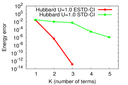
Figure 1: Energy error of 4 sites $U$=1.0 Hubbard model for ESTD (solid line with circle) and STD-CI (broken line with circle).

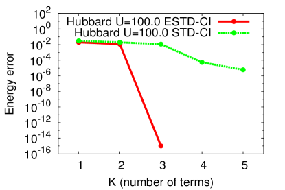
Figure 2: Energy error of 4 sites $U$=100.0 Hubbard model for ESTD (solid line with circle) and STD-CI (broken line with circle).

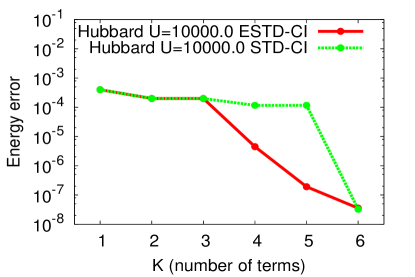
Figure 3: Energy error of 4 sites $U$=10000.0 Hubbard model for ESTD (solid line with circle) and STD-CI (broken line with circle).

Figures 1, 2 and 3 show the total energy referred to the full-CI calculation, or the residual error vs. the tensor rank of the decomposition. The convergence is much faster for ESTD than for STD-CI. For larger $U$ cases, the residual error is initially almost insensitive to the rank and the value amounts to 1-10 when rescaled in unit of $U$. Then the residual error drops suddenly when $K$ is larger than 2 for $U=10^{2}$ and 3 for $U=10^{4}$. This might indicate that the anti-ferromagnetic (AF) ground state cannot be described even at a qualitative level when the number of parameters is unreasonably small. For $U=10^{4}$, the total energy is almost the same among ESTD, STD-CI, and full-CI when the rank is 6. We postulate that the parameter set for STD-CI happens to become suitable for describing the AF limit only at $K\geq 6$.

Table 1 shows detailed comparison of the total energy calculated by AUGP and full-CI for the Hubbard tetramer with $U=10^{2}$. The calculation was done using double precision with $K=3$ . The residual error is $2.2\times 10^{-11}$ while the error was around $10^{-15}$ for ESTD (Fig. (2)); in either scheme the error is close to the double precision limit.

Method	Total energy
AUGP	$-0.119880248924950$
Exact	$-0.119880248946222$

Table 1: Total energy of the Hubbard tetramer with $U=100$ obtained by the AUGP with $K$ = 3. The result obtained by full-CI is also shown.

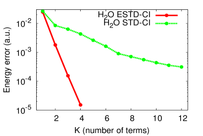
Figure 4: Residual error of the total energy of the H₂O molecule obtained by ESTD (solid line with circle) and STD-CI (broken line with circle).

Figure 4 shows the residual error of the total energy of the H₂O molecule. ESTD shows strikingly faster convergence than STD-CI. In the ESTD and STD-CI calculations, we used quadruple precision since serious loss of significance occurred with double precision. Because of this problem, we could not easily obtain accurate results using $K$ larger than 4 for ESTD, and thus we could not reduce the residual error below $10^{-5}$ Hartree. Figure 5 and Table 2 show the result obtained by using AUGP with double precision. In obtaining the residual error, we used the total energy from full-CI calculation as the reference, but the result is almost the same when using the complete active space self-consistent field (CASSCF) calculation performed using GAUSSIAN09 packageGaussian . The figure shows that the residual energy is reduced almost linearly in log-scale with respect to $K$, indicating an exponential convergence. The table shows that the error is $6.4\times 10^{-3}$ Hartree with $K=4$ and is reduced to $7.2\times 10^{-7}$ Hartree with $K=10$. Although AUGP yields slower convergence than ESTD, the AUGP is very stable. It is not difficult to obtain the optimal parameters $U_{ia}^{r}$ even when the calculation is started from random initial values.

Method	Total energy
AUGP, $K=1$	-61.508355
AUGP, $K=2$	-72.985876
AUGP, $K=3$	-73.457483
AUGP, $K=4$	-75.006008
AUGP, $K=6$	-75.011870
AUGP, $K=8$	-75.012385975
AUGP, $K=10$	-75.012425100
Exact (ours)	-75.012425818
Exact (Gaussian)	-75.012425839

Table 2: Total energy (in unit of Hartree) of H₂O obtained by AUGP. For comparison, the full-CI calculation was done using our own code and the CASSCF calculation using the Gaussian09 package.

Figure 5: Residual error of the total energy of H₂O obtained by AUGP

IV Conclusion

To efficiently represent the CI wavefunction, we have applied the canonical decomposition algorithm to the symmetric part of the CI coefficient. Therein the molecular orbitals are fully optimized, without imposing the orthonormality condition, differently for different terms in the decomposition series. The computational scheme, which we call the extended symmetric tensor decomposition (ESTD), is equivalent to the linear combination of the Hartree-Fock-Bogoliubov states or the linear combination of the antisymmetrized geminal power (AGP). By this, we can rearrange the full-CI series into the canonical decomposition series (STD series). By applying ESTD to the water molecule and Hubbard tetramers, we found that the total energy rapidly converges well within ten terms ($K=10$) for the STD series. The ESTD calculation was found to be numerically unstable when the number of electrons is increased as large as 10 because of the loss of significance in the floating-point arithmetic. This problem could be avoided by restricting the MO coefficients to be complex unitary although the convergence speed with respect to tensor rank $K$ was slightly affected. The computational cost of ESTD scales as $K^{2}M^{5}$ where $M$ is the number of MOs. The result suggests that the AGP-based scheme is a promising computational tool for quantum systems. In this context, it will be an important target of future study to clarify how $K$ depends on the complexity and the size of the system. Our calculation was done without parallelization, but an acceleration by a factor of $K^{2}$ can be expected because of the almost independent nature of the computation. Further acceleration is expected by applying the tensor decomposition scheme to the two-electron integrals as done in Ref.MP2CP ; such technique may possibly reduce the scaling to $K^{2}M^{4}$.

V Acknowledgements

We acknowledge the Strategic Programs for Innovative Research by the Ministry of Education, Culture, Sports, Science and Technology of Japan and the Computational Materials Science Initiative for the financial support during our research. Some of the calculations were performed in the supercomputer facility at the Institute for Solid State Physics, the University of Tokyo. S. K. is supported by Grant-in-Aid for Research Activity Start-up (grant number 25887017) by the Japan Society for the Promotion of Science.

References

- (1) I. Shavitt, Mol. Phys. 94, 3 (1998).
- (2) W. M. C. Foulkes, L. Mitas, R. J. Needs and G. Rajagopal, Rev. Mod. Phys. 73, 33 (2001).
- (3) D. C. Cabra, A. Honecker and P. Pujol, Modern theories of Many-Particle Systems in Condensed Matter Physics (Springer-Verlag, Berlin, Heidelberg, 2012).
- (4) In this paper, we use “order” for the number of indices required to represent a tensor such that a matrix is a tensor of order and use “rank” for the number of terms required for the tensor decomposition.
- (5) T. Neuhauser, M. von Armin and S. D. Peyermhoff, Theor. Chim. Acta. 83, 123 (1992).
- (6) H. Goto, M. Kojo, A. Sasaki and K. Hirose, Nanoscale Res. Lett. 8, 200 (2013).
- (7) R. J. Bartlett and M. Musiał, Rev. Mod. Phys. 79, 291 (2007).
- (8) W. Uemura and O. Sugino, Phys. Rev. Lett. 109, 253001 (2012).
- (9) R. A. Harshman, UCLA Working Papers in Phonetics, 16, 1 (1970).
- (10) J. D. Carroll and J.J. Chang, Psychometrika 35, 283 (1970).
- (11) S. R. White, Phys. Rev. Lett. 69, 2863 (1992).
- (12) S. R. White, Phys. Rev. B 48, 10345 (1993).
- (13) F. Verstraete and J. Cirac, arXiv:cond-mat/0407066 (unpublished); V. Murg, F. Verstraete and J. I. Cirac, Phys. Rev. A 75, 033605 (2007).
- (14) G. K.-L. Chan and M. Head-Gordon, J. Chem. Phys. 116, 4462 (2002).
- (15) N. N. Bogoliubov, Sov. Phys. Usp. 2, 236 (1959), M. Baranger, 1962 Cargese lectures in theoretical physics (Benjamin, New York, 1963).
- (16) A. J. Coleman, Rev. Mod. Phys. 35, 668 (1963).
- (17) A. J. Coleman, J. Math. Phys. 6, 1425 (1965).
- (18) J. V. Ortiz, B. Weiner and Y. Ohn, Int. J. Quantum Chem. 15, 113 (1981).
- (19) V. N. Starovecrov and G. E. Scuseria, J. Chem. Phys. 117, 11107 (2002).
- (20) G. E. Scuseria, C. A. Jimenez-Hoyos, T. M. Henderson, K. Samanta and J. K. Ellis, J. Chem. Phys. 135, 124108 (2011).
- (21) M. Kobayashi, J. Chem. Phys. 140, 084135 (2014).
- (22) B. Weiner and J. V. Ortiz, J. Chem. Phys. 117, 5135 (2002).
- (23) E. Neuscamman, Phys. Rev. Lett. 109, 203001 (2012).
- (24) A. Zen, E. Coccia, Y. Luo, S. Sorella and L. Guidoni, J. Chem. Theory Comput. 10 (3), 1048 (2014).
- (25) D. Taraha and M. Imada, J. Phys. Soc. Jpn. 77, 114701 (2008).
- (26) M. Bajdich, L. Mitas, G. Drobny, L. K. Wagner and K. E. Schmidt, Phys. Rev. Lett. 96, 130201 (2006).
- (27) M. Bajdich, L. Mitas, L. K. Wagner and K. E. Schmidt, Phys. Rev. B 77, 115112 (2008).
- (28) J. J. Griffin and J. A. Wheeler, Phys. Rev. 108, 311 (1957).
- (29) N. Onishi and S. Yoshida, Nucl. Phys. 80, 367 (1966).
- (30) J. Dobaczewski, Phys. Rev. C 62, 017301 (2000).
- (31) T. Mizusaki and M. Oi, Physics Letters B, 715, 219 (2012).
- (32) K. Neergård and W. Wüst, Nucl. Phys. A 402, 311 (1983).
- (33) C. G. Broyden, J. lnst. Maths. Appl. 6, 76 (1970).
- (34) R. Fletcher, Comp. J. 13, 317 (1970).
- (35) D. Goldfarb, Math. Comp. 24, 23 (1970).
- (36) D. F. Shanno, Math Comp. 24, 647 (1970).
- (37) R. Fletcher, in Practical methods of optimization, Vol. 1 (Wiley, New York, 1980).
- (38) C. Bloch and A. Messiah, Nucl. Phys. 39, 95 (1962).
- (39) Gaussian 09, M. J. Frisch, G. W. Trucks, H. B. Schlegel, G. E. Scuseria, M. A. Robb, J. R. Cheeseman, G. Scalmani, V. Barone, B. Mennucci, G. A. Petersson, H. Nakatsuji, M. Caricato, X. Li, H. P. Hratchian, A. F. Izmaylov, J. Bloino, G. Zheng, J. L. Sonnenberg, M. Hada, M. Ehara, K. Toyota, R. Fukuda, J. Hasegawa, M. Ishida, T. Nakajima, Y. Honda, O. Kitao, H. Nakai, T. Vreven, J. A. Montgomery, Jr., J. E. Peralta, F. Ogliaro, M. Bearpark, J. J. Heyd, E. Brothers, K. N. Kudin, V. N. Staroverov, R. Kobayashi, J. Normand, K. Raghavachari, A. Rendell, J. C. Burant, S. S. Iyengar, J. Tomasi, M. Cossi, N. Rega, J. M. Millam, M. Klene, J. E. Knox, J. B. Cross, V. Bakken, C. Adamo, J. Jaramillo, R. Gomperts, R. E. Stratmann, O. Yazyev, A. J. Austin, R. Cammi, C. Pomelli, J. W. Ochterski, R. L. Martin, K. Morokuma, V. G. Zakrzewski, G. A. Voth, P. Salvador, J. J. Dannenberg, S. Dapprich, A. D. Daniels, Ö. Farkas, J. B. Foresman, J. V. Ortiz, J. Cioslowski and D. J. Fox, Gaussian, Inc., Wallingford CT (2009).
- (40) U. Benedikt, A. A. Auer, M. Espig and W. Hackbusch, J. Chem. Phys. 134, 054118 (2011).