A Computable Measure of Algorithmic Probability by Finite Approximations with an Application to Integer Sequences
Abstract
Given the widespread use of lossless compression algorithms to approximate algorithmic (Kolmogorov-Chaitin) complexity, and that, usually, generic lossless compression algorithms fall short at characterizing features other than statistical ones not different to entropy evaluations, here we explore an alternative and complementary approach. We study formal properties of a Levin-inspired measure calculated from the output distribution of small Turing machines. We introduce and justify finite approximations that have been used in some applications as an alternative to lossless compression algorithms for approximating algorithmic (Kolmogorov-Chaitin) complexity. We provide proofs of the relevant properties of both and and compare them to Levin’s Universal Distribution. We provide error estimations of with respect to . Finally, we present an application to integer sequences from the Online Encyclopedia of Integer Sequences which suggests that our AP-based measures may characterize non-statistical patterns, and we report interesting correlations with textual, function and program description lengths of the said sequences.
Keywords: Kolmogorov-Chaitin complexity, algorithmic probability, algorithmic Coding Theorem, Turing machines, integer sequences
1 Algorithmic information measures
Central to Algorithmic Information Theory is the definition of algorithmic (Kolmogorov-Chaitin or program-size) complexity [10, 2]:
| (1) |
where is a program that outputs running on a universal Turing machine and is the length in bits of . The measure was first conceived to define randomness and is today the accepted objective mathematical measure of randomness, among other reasons because it has been proven to be mathematically robust [11]. In the following, we use instead of because the choice of is only relevant up to an additive constant (Invariance Theorem). A technical inconvenience of as a function taking to be the length of the shortest program that produces is its uncomputability. In other words, there is no program which takes a string as input and produces the integer as output. This is usually considered a major problem, but one ought to expect a universal measure of randomness to have such a property.
In previous papers [5, 16] we have introduced a novel method to approximate based on the seminal concept of algorithmic probability (or AP), introduced by Solomonoff [18] and further formalized by Levin [11], who proposed the concept of uncomputable semi-measures and the so-called Universal Distribution.
Levin’s semi-measure111It is called a semi measure because, unlike probability measures, the sum is never 1. This is due to the Turing machines that never halt. defines the so-called Universal Distribution [9], the value being the probability that a random program halts and produces running on a universal Turing machine . The choice of is only relevant up to a multiplicative constant, so we will simply write instead of .
It is possible to use to approximate by means of the following theorem:
Theorem 1 (Algorithmic Coding Theorem [11]).
There is a constant such that
| (2) |
This implies that if a string has many descriptions (high value of , as the string is produced many times, which implies a low value of , given that ), it also has a short description (low value of ). This is because the most frequent strings produced by programs of length are those which were already produced by programs of length , as extra bits can produce redundancy in an exponential number of ways. On the other hand, strings produced by programs of length that could not be produced by programs of length are less frequently produced by programs of length , as only very specific programs can generate them (see Section 14.6 in [3]). This theorem elegantly connects probability to complexity—the frequency (or probability) of occurrence of a string with its algorithmic (Kolmogorov-Chaitin) complexity. It implies that [5] one can calculate the Kolmogorov complexity of a string from its frequency [5], simply rewriting the formula as:
| (3) |
Thanks to this elegant connection established by (2) between algorithmic complexity and probability, our method can attempt to approximate an algorithmic probability measure by means of finite approximations using a fixed model of computation. The method is called the Coding Theorem Method (CTM) [16].
In this paper we introduce , a computable approximation to that can be used to approximate by means of the algorithmic Coding theorem. Computing requires the output of a numerable infinite number of Turing machines, so we first undertake the investigation of finite approximations that require only the output of machines up to states. A key property of and is their universality: the choice of the Turing machine used to compute the distribution is only relevant up to an (additive) constant, independent of the objects. The computability of this measure implies its lack of universality. The same is true when using common lossless compression algorithms to approximate , but on top of their non-universality in the algorithmic sense, they are block entropy estimators as they traverse files in search of repeated patterns in a fixed-length window to build a replacement dictionary. Nevertheless, this does not prevent lossless compression algorithms to find useful applications in the same way as more algorithmic-based motivated measures can contribute even if also limited. Indeed, has found successful applications in cognitive sciences [15, 14, 6, 7, 8], in financial time series research [20, 12], graph theory and networks [23, 24, 26]. However, a thorough investigation to explore the properties of these measures, and to provide theoretical error estimations was missing.
We start by presenting our Turing machine formalism (Section 2) and then show that it can be used to encode a prefix-free set of programs (Section 3). Then, in Section 4 we define a computable algorithmic probability measure based on our Turing machine formalism and prove its main properties, both for and for finite approximations . In Section 5 we compute , compare it with our previous distribution [16] and estimate the error in as an approximation to . We finish with some comments in Section 7.
2 The Turing machine formalism
We denote by the class (or space) of all -state 2-symbol Turing machines (with the halting state not included among the states) following the Busy Beaver Turing machine formalism as defined by Rado [13]. Busy Beaver Turing machines are deterministic machines with a single head and a single tape unbounded in both directions. When the machine enters the halting state the head no longer moves and the output is considered to comprise only the cells visited by the head prior to halting. Formally,
Definition 2 (Turing machine formalism).
We designate as the set of Turing machines with two symbols and states plus a halting state . These machines have entries (for and ) in the transition table, each with one instruction that determines their behavior. Such entries are represented by
| (4) |
where and are respectively the current state and the symbol being read and represents the instruction to be executed: is the new state, the symbol to write and the direction. If is the halting state , then , otherwise is (right) or (left).
Proposition 3.
Machines in can be enumerated from to
Proof.
Given the constraints in Definition 2, for each transition of a Turing machine in there are different instructions . These are instructions when (given that is fixed and can be one of the two possible symbols) and instructions if ( possible moves, states and symbols). Then, considering the entries in the transition table,
| (5) |
These machines can be enumerated from to . Several enumerations are possible. We can, for example, use a lexicographic ordering on the transitions (4). ∎
For the current paper, consider that some enumeration has been chosen. Thus we use to denote the machine number in following that enumeration.
3 Turing machines as a prefix-free set of programs
We show in this section that the set of Turing machines following the Busy Beaver formalism can be encoded as a prefix-free set of programs capable of generating any finite non-empty binary string.
Definition 4 (Execution of a Turing machine).
Let be a Turing machine. We denote by the execution of over an infinite tape filled with (a blank symbol), where . We write if halts, and otherwise. We write iff
-
•
, and
-
•
is the output string of , defined as the concatenation of the symbols in the tape of that were visited at some instant of the execution .
As Definition 4 establishes, we are only considering machines running over a blank tape with no input. Observe that the output of considers the symbols in all cells of the tape written on by during the computation, so the output contains the entire fragment of the tape that was used. To produce a symmetrical set of strings, we consider both symbols and as possible blank symbols.
Definition 5 (Program).
A program is a triplet , where
-
•
is a natural number
-
•
-
•
We say that the output of is if, and only if, .
Programs can be executed by a universal Turing machine that reads a binary encoding of (Definition 6) and simulates . Trivially, for each finite binary string with length , there is a program which outputs .
Now that we have a formal definition of programs, we show that the set of valid programs can be represented as a prefix-free set of binary strings.
Definition 6 (Binary encoding of a program).
Let be a program (Definition 5). The binary encoding of is a binary string with the following sequence of bits:
-
•
First, , that is, repetitions of followed by . This way we encode .
-
•
Second, a bit with value encodes the blank symbol.
-
•
Finally, is encoded using bits.
The use of bits to represent ensures that all programs with the same are represented by strings of equal size. As there are machines in , with these bits we can represent any value of . The process of reading the binary encoding of a program and simulating is computable, given the enumeration of Turing machines.
As an example, this is the binary representation of the program :
| 1 | 0 | 0 | 0 | 0 | 0 | 0 | 0 | 0 | 1 | 0 | 1 | 1 | 1 | 0 | 0 | 1 |
|---|
The proposed encoding is prefix-free, that is, there is no pair of programs , such that the binary encoding of is a prefix of the binary encoding of . This is because the initial bits of the binary encoding of determine the length of the encoding. So cannot be encoded by a binary string having a different length but the same initial bits.
Proposition 7 (Programming by coin flips).
Every source producing an arbitrary number of random bits generates a unique program (provided it generates at least one ).
Proof.
The bits in the sequence are used to produce a unique program following Definition 6. We start by producing the first part, by selecting all bits until the first appears. Then the next bit gives . Finally, as we know the value of , we take the following bits to set the value of . It is possible that constructing the program in this way, the value of is greater than the maximum in the enumeration. In which case we associate the program with some trivial non-halting Turing machine. For example a machine with the initial transition staying at the initial state. ∎
The idea of programming by coin flips is very common in Algorithmic Information Theory. It produces a prefix-free coding system, that is, there is no string encoding a program which is a prefix of a string encoding a program . These coding systems make longer programs (for us, Turing machines with more states) exponentially less probable than short programs. In our case, this is because of the initial sequence of repetitions of , which are produced with probability . This observation is important because when we later use machines in to reach a finite approximation of our measure, the greater is, the exponentially smaller the error we will be allowing: the probability of producing by coin flips a random Turing machine with more than states decreases exponentially with [3].
4 A Levin-style algorithmic measure
Definition 8.
Given a Turing machine accepting a prefix-free set of programs, the probability distribution of is defined as
| (6) |
where is equal to if and only if halts with input and produces . The length in bits of program is represented by .
If is a universal Turing machine, measures how frequently the output is generated when running random programs at . Given that the sum of for all strings is not (non-halting programs not producing any strings are counted in ) it is said to be a semi-measure, also known as Levin’s distribution [11]. The distribution is universal in the sense that the choice of (among all the infinite possible universal reference Turing machines) is only relevant up to a multiplicative constant and that the distribution is based on the universal model of Turing computability.
Definition 9 (Distribution ).
Let be a Turing machine executing the programs introduced in Definition 5. Then, is defined by
Theorem 10.
For any binary string ,
| (7) |
Proof.
By Definition 6, the length of the encoding of program is . It justifies the denominator of (7), as (6) requires it to be . For the numerator, observe that the set of programs producing with the same value corresponds to all machines in producing with either or as blank symbol. Note that if a machine produces both with and , it is counted twice, as each execution is represented by a different program (that differ only as to the digit). ∎
4.1 Finite approximations to
The value of for any string depends on the output of an infinite set of Turing machines, so we have to manage ways to approximate it. The method proposed in Definition 11 approximates by considering only a finite number of Turing machines up to a certain number of states.
Definition 11 (Finite approximation ).
The finite approximation to bound to states, , is defined as
| (8) |
Proposition 12 (Convergence of to ).
Proposition 12 ensures that the sum of the error in as an approximation to , for all strings , decreases exponentially with . The question of this convergence was first broached in [4]. The bound of has only theoretical value; in practice we can find lower bounds. In fact, the proof counts all programs of size to bound the error (and many of them do not halt). In Section 5.1 we provide a finer error calculation for by removing from the count some very trivial machines that do not halt.
4.2 Properties of and
Levin’s distribution is characterized by some important properties. First, it is lower semi-computable, that is, it is possible to compute lower bounds for it. Also, it is a semi-measure, because the sum of probabilities for all strings is smaller than . The key property of Levin’s distribution is its universality: a semi-measure is universal if and only if for every other semi-measure there exists a constant (that may depend only on and ) such that for every string , . That is, a distribution is universal if and only if it dominates (modulo a multiplicative constant) every other semi-measure. In this section we present some results pertaining to the computational properties of and .
Proposition 13 (Runtime bound).
Given any binary string , a machine with states producing runs a maximum of steps upon halting or never halts.
Proof.
Suppose that a machine produces . We can trace back the computation of upon halting by looking at the portion of cells in the tape that will constitute the output. Before each step, the machine may be in one of possible states, reading one of the cells. Also, the cells can be filled in ways (with a or in each cell). This makes for different possible instantaneous descriptions of the computation. So any machine may run, at most, that number of steps in order to produce . Otherwise, it would produce a string with a greater length (visiting more than cells) or enter a loop.
∎
Observe that a key property of our output convention is that we use all visited cells in the machine tape. This is what gives us the runtime bound which serves to prove the most important property of , its computability (Theorem 14).
Theorem 14 (Computability of ).
Given and , the value of is computable.
Proof.
According to (8) and Proposition 3, there is a finite number of machines involved in the computation of . Also, Proposition 13 sets the maximum runtime for any of these machines in order to produce . So an algorithm to compute enumerates all machines in , and runs each machine to the corresponding bound. ∎
Corollary 15.
Given a binary string , the minimum with is computable.
Proof.
Trivially, can be produced by a Turing machine with states in just steps. At each step , this machine writes the th symbol of , moves to the right and changes to a new state. When all symbols of have been written, the machine halts. So, to get the minimum with , we can enumerate all machines in , and run all of them up to the runtime bound given by Proposition 13. The first machine producing (if the machines are enumerated from smaller to larger size) gives the value of . ∎
Now, some uncomputability results of
Proposition 16.
Given , the length of the longest with is non-computable.
Proof.
We proceed by contradiction. Suppose that such a computable function as gives the length of the longest with . Then ?, together with the runtime bound in Proposition 13, provides a computable function that gives the maximum runtime that a machine in may run prior to halting. But it contradicts the uncomputability of the Busy Beaver [13]: the highest runtime of halting machines in grows faster than any computable function. ∎
Corollary 17.
Given , the number of different strings with is non-computable.
Proof.
Also by contradiction: If the number of different strings with is computable, we can run in parallel all machines in until the corresponding number of different strings has been found. This gives us the longest string, which is in contradiction to Proposition 16. ∎
Now to the key property of , its computability,
Theorem 18 (Computability of ).
Given any non-empty binary string, is computable.
Proof.
As we argued in the proof of Corollary 15, a non-empty binary string can be produced by a machine with states. Trivially, it is then also produced by machines with more than states. So for every non-empty string , the value of , according to (7), is the sum of enumerable infinite many rationals which produce a real number. A real number is computable if, and only if, there is some algorithm that, given , returns the first digits of the number. And this is what does. Proposition 12 enables us to calculate the value of such that provides the required digits of , as is bounded by . ∎
The subunitarity of and implies that the sum of (or ) for all strings is smaller than one. This is because of the non-halting machines:
Proposition 19 (Subunitarity).
The sum of for all strings is smaller than , that is,
Proof.
By using (7),
| (9) |
but is the number of machines in that halt when starting with a blank tape filled with plus the number of machines in that halt when starting on a blank tape filled with . This number is at most twice the cardinality of , but we know that it is smaller, as there are very trivial machines that do not halt, such as those without transitions to the halting state, so
∎
Corollary 20.
The sum of for all strings is smaller than
The key property of and is their computability, given by Propositions 14 and 18, respectively. So these distributions cannot be universal, as Levin’s Universal Distribution is non-computable. In spite of this, the computability of our distributions (and the possibility of approximating them with a reasonable computational effort), as we have shown, provides us with a tool to approximate the algorithmic probability of short binary strings. In some sense this is similar to what happens with other (computable) approximations to (uncomputable) Kolmogorov complexity, such as common lossless compression algorithms, which in turn are estimators of the classical Shannon entropy rate (e.g. all those based in LZW, and unlike and , are not able to find algorithmic content beyond statistical patterns, not even in principle, unless a compression algorithm is designed to seek a specific one. For example, the digital expansion of the mathematical constant is believed to be normal and therefore will contain no statistical patterns of the kind that compression algorithms can detect, yet there will be a (short) computer program that can generate it, or at least finite (and small) initial segments of .
5 Computing
We have explored the sets of Turing machines in for in previous papers [5, 16]. For , the maximum time that a machine in may run upon hating is known [1]. It allows us to calculate the exact values of . For , we have estimated [16] that 500 steps cover almost the totality of halting machines. We have the database of machines producing each string for each value of . So we have applied (8) to estimate (because we set a low runtime).
In previous papers [16, 17], we worked with , a measure similar to , but the denominator of (8) is the number of (detected) halting machines in . Using as an approximation to Levin’s distribution, algorithmic complexity is estimated222These values can be consulted at http://www.complexitycalculator.com. Accessed on June 22, 2017. by means of the algorithmic Coding Theorem 1 as . Now, provides us with another estimation: . Table 1 shows the 10 most frequent strings in both distributions, together with their estimated complexity.
| 0 | 3.7671 | 2.5143 | 11 | 6.8255 | 3.3274 |
|---|---|---|---|---|---|
| 1 | 3.7671 | 2.5143 | 000 | 10.4042 | 5.3962 |
| 00 | 6.8255 | 3.3274 | 111 | 10.4042 | 5.3962 |
| 01 | 6.8255 | 3.3274 | 001 | 10.4264 | 5.4458 |
| 10 | 6.8255 | 3.3274 | 011 | 10.4264 | 5.4458 |
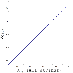
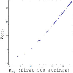
Figure 1 shows a rank comparison of both estimations of algorithmic complexity after application of the algorithmic Coding Theorem. With minor differences, there is an almost perfect agreement. So in classifying strings according to their relative algorithmic complexity, the two distributions are equivalent.
The main difference between and is that is not computable, because computing it would require us to know the exact number of halting machines in , which is impossible given the halting problem. We work with approximations to by considering the number of halting machines detected. In any case, though is computable, it is computationally intractable, so in practice (approximations to) the two measures can be used interchangeably .
5.1 Error calculation
We can make some estimations about the error in with respect to . “0” and “1” are two very special strings, both with the maximum value. These strings are the most frequent outputs in for , and we may conjecture that they are the most frequent outputs for all values of . These strings then have the greatest absolute error, because the terms in the sum of (the argument for is identical) not included in are always the greatest independent of .
We can calculate the exact value of the terms for in (7). To produce “0”, starting with a tape filled with , a machine in must have the transition corresponding to the initial state and read symbol with the following instruction: write and change to the halting state (thus not moving the head). The other transitions may have any of the possible instructions. So there are machines in producing “0” when running on a tape filled with . Considering both values of , we have programs of the same length producing “0”. Then, for “0”,
| (10) |
This can be approximated by
we have divided the infinite sum into two intervals cutting at 2000 because the approximation of to is not good for low values of , but has almost no impact for large . In fact, cutting at 1000 or 4000 gives the same result with a precision of 17 decimal places. We have used Mathematica to calculate both the sum from to and the convergence from to infinity. So the value is exact for practical purposes. The value of is , so the error in the calculation of is . If “0” and “1” are the strings with the highest value, as we (informedly) conjecture, then this is the maximum error in as an approximation to .
As a reference, is . With the real value, the approximated complexity is . The difference is not relevant for most practical purposes.
We can also provide an upper bound for the sum of the error in for strings different from “0” and “1”. Our way of proceeding is similar to the proof of Proposition 12, but we count in a finer fashion. The sum of the error for strings different from “0” and “1” is
| (11) |
The numerators of the above sum contain the number of computations (with blank symbol “0” or “1”) of Turing machines in , , that halt and produce an output different from “0” and “1”. We can obtain an upper bound of this value by removing, from the set of computations in , those that produce “0” or “1” and some trivial cases of machines that do not halt.
First, the number of computations in is , as all machines in are run twice for both blank symbols (“0” and “1”). Also, the computations producing “0” or “1” are . Now, we focus on two sets of trivial non-halting machines:
-
•
Machines with the initial transition staying at the initial state. For blank symbol , there are machines that when reading at the initial state do not change the state (for the initial transition there are possibilities, depending on the writing symbol and direction, and for the other transitions there are possibilities). These machines will keep moving in the same direction without halting. Considering both blank symbols, we have computations of this kind.
-
•
Machines without transition to the halting state. To keep the intersection of this and the above set empty, we also consider that the initial transition moves to a state different from the initial state. So for blank symbol , we have different initial transitions ( directions, writing symbols and states) and different possibilities for the other transitions. This makes a total of different machines for blank symbol and computations for both blank symbols.
Now, an upper bound for (11) is:
The result of the above sum is (smaller than , as guaranteed by Proposition 12). This is an upper bound of the sum of the error for all infinite strings different from “0” and “1”. Smaller upper bounds can be found by removing from the above sum other kinds of predictable non-halting machines.
6 Algorithmic Complexity of Integer Sequences
Measures that we introduced based on finite approximations of algorithmic probability have found applications in areas ranging from economics [20] to human behavior and cognition [7, 8, 15] to graph theory [23]. We have explored the use of other models of computation suggesting similar and correlated results in output distribution [19] and compatibility, in a range of applications, with general compression algorithms [17, 21]. We also investigated [16] the behavior of the additive constant involved in the Invariance theorem from finite approximations to , strongly suggesting fast convergence and smooth behavior of the invariance constant. In [23] and [21], we introduced an AP-based measure for 2-dimensional patterns, based on replacing the tape of the reference Turing machine for a 2-dimensional grid. The actual implementation requires breaking any grid into smaller blocks for which we then have estimations of their algorithmic probability according to the Turing machine formalism described in [25, 23] and [21].
Here we introduce an application of AP-based measures–as described above–to integer sequences. We show that an AP-based measure constitutes an alternative or complementary tool to lossless compression algorithms, widely used to find estimations of algorithmic complexity.
6.1 AP-based measure
The AP-based method used here is based on the distribution and is defined just like . However, to increase its range of applicability, given that produces all bit-strings of length 12 except for 2 (that are assigned maximum values and thus complete the set), we introduce what we call the Block Decomposition Method (BDM) that decomposes strings longer than 12 into strings of maximum length 12 that can be derived from . The final estimation of the complexity of a string longer than 12 bits is then the result of the sum of the complexities of the different substrings of length not exceeding 12 in if they are different, but the sum of only if substrings are the same. The formula is motivated by the fact that strings that are the same do not have times the complexity of one of the strings but rather times the complexity of just one of the substrings. This is because the algorithmic complexity of the substrings to be considered is the length of at most the ‘print() times’ program and not the length of ‘print()’. We have shown that this measure is a hybrid measure of complexity, providing local estimations of algorithmic complexity and global evaluations of Shannon entropy [25]. Formally,
where is the multiplicity of , and the subsequences from the decomposition of into subsequences, with a possible remainder sequence if is not a multiple of the decomposition length . More details on error estimations for this particular measure extending the power of , and on the boundary conditions, are given in [25].
6.2 The On-Line Encyclopedia of Integer Sequences (OEIS)
The On-Line Encyclopedia of Integer Sequences (OEIS) is a database with the largest collection of integer sequences. It is created and maintained by Neil Sloane and the OEIS Foundation.
Widely cited, the OEIS stores information on integer sequences of interest to both professional mathematicians and amateurs. As of 30 December 2016 it contained nearly 280 000 sequences, making it the largest database of its kind.
We found 875 binary sequences in the OEIS database, accessed through the knowledge engine WolframAlpha Pro and downloaded with the Wolfram Language.
Examples of descriptions found to have the greatest algorithmic probability include the sequence “A maximally unpredictable sequence” with associated sequence 0 1 0 0 1 1 0 1 0 1 1 1 0 0 0 1 0 0 0 0 1 1 1 1 0 1 1 0 0 1 0 1 0 0 1 0 0 1 1 1; or A068426, the “Expansion of in base 2” and associated sequence 0 1 0 0 0 1 1 0 1 1 0 0 0 0 0 1 0 1 0 0 1 1 1 0 0 1 0 1 1 1 0 1 1 1 0 0 0 0 0 0. This contrasts with sequences of high entropy such as sequence A130198, the single paradiddle, a four-note drumming pattern consisting of two alternating notes followed by two notes with the same hand, with sequence 0 1 0 0 1 0 1 1 0 1 0 0 1 0 1 1 0 1 0 0 1 0 1 1 0 1 0 0 1 0 1 1 0 1 0 0 1 0 1 1, or sequence A108737, found to be among the less compressible, with the description “Start with . For let be the binary expansion of . If is not a substring of , append the minimal number of 0s and 1s to to remedy this. The sequence gives ” and sequence 0 1 0 1 1 0 0 1 1 1 0 0 0 1 0 1 0 1 1 0 1 1 1 1 0 0 0 0 1 0 0 1 0 1 0 0 1 1 0 1. We found that the measure most driven by description length was compressibility.
The longest description of a binary sequence in the OEIS, identified as A123594, reads “Unique sequence of 0s and 1s which are either repeated or not repeated with the following property: when the sequence is ‘coded’ in writing down a 1 when an element is repeated and a 0 when it is not repeated and by putting the initial element in front of the sequence thus obtained, the above sequence appears”.
6.3 Results
We found that the textual description length as derived from the database is, as illustrated above, best correlated with the AP-based (BDM) measure, with Spearman test statistic 0.193, followed by compression (only the sequence is compressed, not the description) with 0.17, followed by entropy, with 0.09 (Fig. 2). Spearman rank correlation values among complexity measures reveal how these measures are related to each other with BDM v Compress: 0.21, BDM v Entropy: 0.029 and Compress v Entropy: -0.01 from 875 binary sequences in the OEIS database.
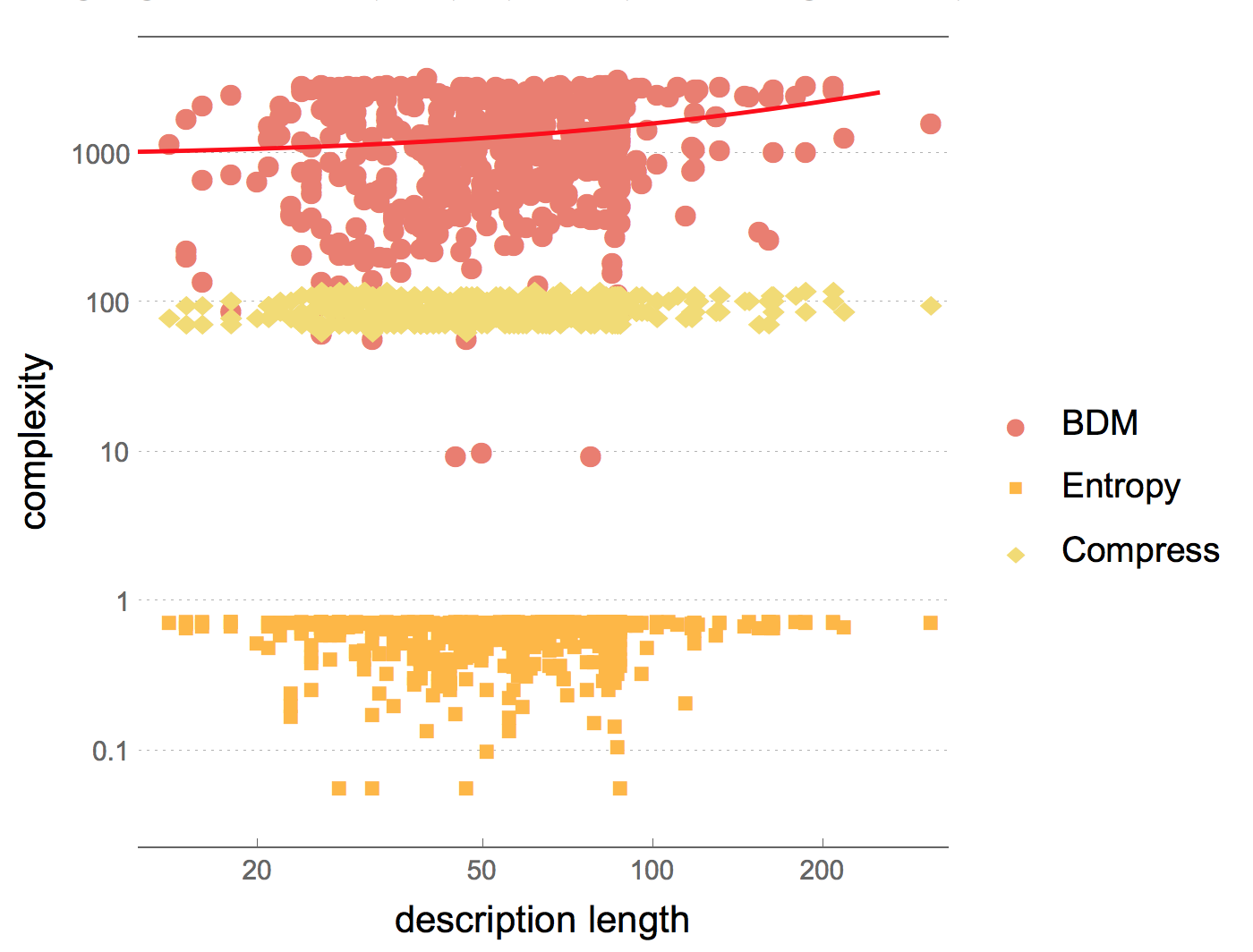
We noticed that the descriptions of some sequences referred to other sequences to produce a new one (e.g. “A051066 read mod 2”). This artificially made some sequence descriptions look shorter than they should be. When avoiding all sequences referencing others, all Spearman rank values increased significantly, with values 0.25, 0.22 and 0.12 for BDM, compression and entropy respectively.
To test whether the AP-based (BDM) measure captures some algorithmic content that the best statistical measures (Compress and entropy) may be missing, we compressed the sequence description and compared again against the sequence complexity. The correlation between the compressed description and the sequence compression came closer to that of the AP-estimation by BDM, and BDM itself was even better. The Spearman values after compressing textual descriptions were 0.27, 0.24 and 0.13 for BDM, Compress and entropy respectively.
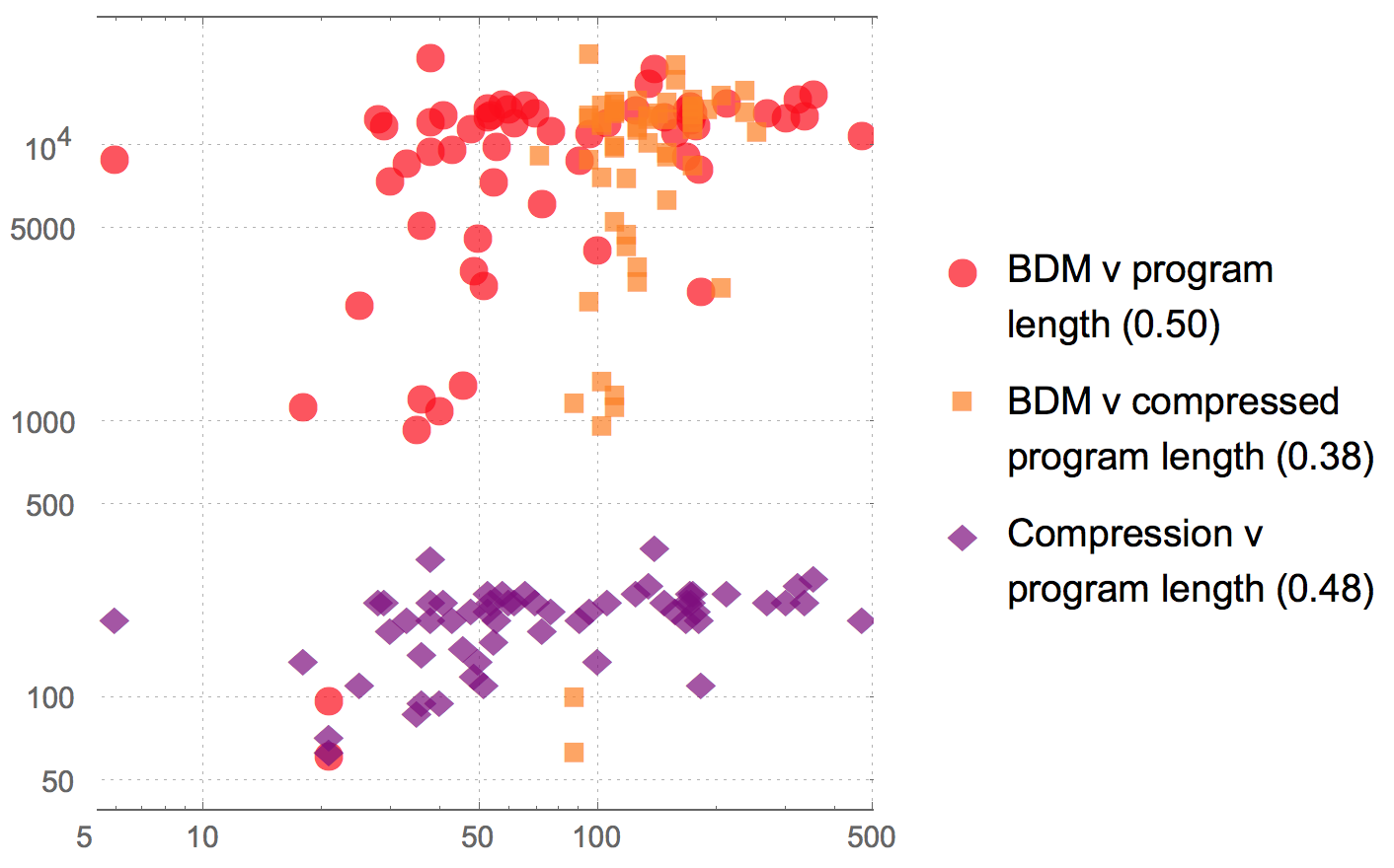
We then looked at 139 546 integer sequences from the OEIS database, avoiding other non-integer sequences in the database. Those considered represent more than half of the database. Every integer was converted into binary, and for each binary sequence representing an integer an estimation of its algorithmic complexity was calculated. We compared the total sum of the complexity of the sequence (first 40 terms) against its text description length (both compressed and uncompressed) by converting every character into its ASCII code, program length and function lengths, these latter in the Wolfram Language (using Mathematica). While none of those descriptions can be considered the shortest possible, their lengths are upper bounds of the maximum possible lengths of the shortest versions. As shown in Fig. 2, we found that the AP-based measure (BDM) performed best when comparing program size and estimated complexity from the program-generated sequence.
7 Conclusion
Computable approximations to algorithmic information measures are certainly useful. For example, lossless compression methods have been widely used to approximate , despite their limitations and their departure from algorithmic complexity. Most of these algorithms are in fact entropy-rate estimators [22] e.g. all those based in LZ and LZW algorithms such as zip, gzip and png. In this paper we have studied the formal properties of a computable algorithmic probability measure and of finite approximations to . These measures can be used to approximate by means of the Coding Theorem Method (CTM), despite the invariance theorem, that sheds no light on the rate of convergence to . Here we compared and and concluded that for practical purposes the two produce similar results. What we have reported in this paper are the first steps toward a formal analysis of finite approximations to algorithmic probability-based measures based on small Turing machines. The results shown in Fig. 2 strongly suggest that AP-based measures are not only an alternative to lossless compression algorithms for estimating algorithmic (Kolmogorov-Chaitin) complexity, but may actually capture features that statistical methods such as lossless compression, based on popular algorithms such as LWZ and entropy, cannot capture.
Acknowledgments
The authors wish to thank the rest of the Algorithmic Nature lab.
References
- [1] A.H. Brady, The determination of the value of Rado’s noncomputable function for four-state Turing machines, Mathematics of Computation 40 (162): 647–665, 1983.
- [2] G.J. Chaitin, On the length of programs for computing finite binary sequences: Statistical considerations, Journal of the ACM, 16(1):145–159, 1969.
- [3] T.M. Cover, J.A. Thomas, Elements of Information Theory, Wiley Series in Telecommunications and Signal Processing, Wiley-Blackwell; 2nd. Edition ed., 2006.
- [4] J-P. Delahaye, H. Zenil, Towards a stable definition of Kolmogorov-Chaitin complexity, arXiv:0804.3459, 2007 (preprint).
- [5] J.-P. Delahaye & H. Zenil, Numerical Evaluation of the Complexity of Short Strings: A Glance Into the Innermost Structure of Algorithmic Randomness, Applied Math. and Comp., 2012.
- [6] N. Gauvrit, H. Singmann, F. Soler-Toscano, H. Zenil, Algorithmic complexity for psychology: A user-friendly implementation of the coding theorem method, Behavior Research Methods, 2015 (in press).
- [7] N. Gauvrit, F. Soler-Toscano, H. Zenil, Natural scene statistics mediate the perception of image complexity, Visual Cognition, vol. 22:8, pp.1084–1091, 2014.
- [8] V. Kempe, N. Gauvrit, D. Forsyth, Structure emerges faster during cultural transmission in children than in adults, Cognition, Cognition vol. 136, pp 247–254, 2015.
- [9] W. Kircher, M. Li, and P. Vitanyi, The Miraculous Universal Distribution, The Mathematical Intelligencer, 19:4, 7–15, 1997.
- [10] A.N. Kolmogorov, Three approaches to the quantitative definition of information, Problems of Information and Transmission, 1(1):1–7, 1965.
- [11] L. Levin, Laws of information conservation (non-growth) and aspects of the foundation of probability theory, Problems in Form. Transmission 10. 206–210, 1974.
- [12] L. Ma, O. Brandouy, J.-P. Delahaye and H. Zenil, Algorithmic Complexity of Financial Motions, Research in International Business and Finance, pp. 336-347, 2014.
- [13] T. Radó, On non-computable functions, Bell System Technical Journal, Vol. 41, No. 3, pp. 877–884, 1962.
- [14] N. Gauvrit, H. Zenil, J.-P. Delahaye and F. Soler-Toscano Algorithmic complexity for short binary strings applied to psychology: a primer, Behavior Research Methods, vol. 46, Issue 3, 2014, pp. 732–744.
- [15] N. Gauvrit, H. Zenil, F. Soler-Toscano, J.-P. Delahaye, P. Brugger, Human Behavioral Complexity Peaks at Age 25, PLoS Comput Biol 13(4): e1005408, 2017.
- [16] F. Soler-Toscano, H. Zenil, J.-P. Delahaye and N. Gauvrit, “Calculating Kolmogorov Complexity from the Output Frequency Distributions of Small Turing Machines”, PLoS ONE 9(5): e96223.
- [17] F. Soler-Toscano, H. Zenil, J.-P. Delahaye and N. Gauvrit, Correspondence and Independence of Numerical Evaluations of Algorithmic Information Measures, Computability, vol. 2, number 2 (2013), pp. 125–140.
- [18] R.J. Solomonoff, A formal theory of inductive inference: Parts 1 and 2. Information and Control, 7:1–22 and 224–254, 1964.
- [19] H. Zenil and J-P. Delahaye, On the Algorithmic Nature of the World, In G. Dodig-Crnkovic and M. Burgin (eds), Information and Computation, World Scientific Publishing Company, 2010.
- [20] H. Zenil and J.-P. Delahaye, An Algorithmic Information-theoretic Approach to the Behaviour of Financial Markets, Journal of Economic Surveys, vol. 25-3, pp. 463, 2011.
- [21] H. Zenil, F. Soler-Toscano, J.-P. Delahaye and N. Gauvrit, Two-Dimensional Kolmogorov Complexity and Validation of the Coding Theorem Method by Compressibility, PeerJ Comput. Sci., 1:e23, 2015.
- [22] H. Zenil, Algorithmic Data Analytics, Small Data Matters and Correlation versus Causation. In Max Ott, Wolfgang Pietsch, Jörg Wernecke (eds.) Berechenbarkeit der Welt? Philosophie und Wissenschaft im Zeitalter von Big Data (Computability of the World? Philosophy and Science in the Age of Big Data), Springer Verlag, Heidelberg, 2017.
- [23] H. Zenil, F. Soler-Toscano, K. Dingle and A. Louis, Correlation of automorphism group size and topological properties with program-size complexity evaluations of graphs and complex networks, Physica A: Statistical Mechanics and its Applications, Volume 404, pp. 341–358, 2014.
- [24] H. Zenil, N.A. Kiani and J. Tegnér, Methods of Information Theory and Algorithmic Complexity for Network Biology, Seminars in Cell and Developmental Biology, vol. 51, pp. 32-43, 2016.
- [25] H. Zenil, F. Soler-Toscano, N.A. Kiani, S. Hernández-Orozco, A. Rueda-Toicen, A Decomposition Method for Global Evaluation of Shannon Entropy and Local Estimations of Algorithmic Complexity, arXiv:1609.00110 [cs.IT].
- [26] H. Zenil, N.A. Kiani and Jesper Tegnér, Low Algorithmic Complexity Entropy-deceiving Graphs, Phys Rev E. (in press).