Elastoconductivity as a probe of broken mirror symmetries

Abstract

We propose the possible detection of broken mirror symmetries in correlated two-dimensional materials by elastotransport measurements. Using linear response theory we calculate the“shear conductivity” $\Gamma_{xx,xy}$, defined as the linear change of the longitudinal conductivity $\sigma_{xx}$ due to a shear strain $\epsilon_{xy}$. This quantity can only be non-vanishing when in-plane mirror symmetries are broken and we discuss how candidate states in the cuprate pseudogap regime (e.g. various loop current or charge orders) may exhibit a finite shear conductivity. We also provide a realistic experimental protocol for detecting such a response.

I Introduction

Phases of matter in solids are often empirically distinguished by their transport properties. Electrical transport measurements probe long wavelength properties of the system, and in metallic phases, they are sensitive to electronic excitations near the Fermi level. In addition, these measurements often exhibit singular features at phase transitions, thus indicating the onset of broken symmetries. However, aside from a few instances such as the anomalous Hall effect in ferromagnets, the exact form of the broken symmetry is not usually evident from a transport measurement. Experiments that aid in directly identifying subtle forms of broken symmetry are therefore invaluable in the study of strongly correlated electron materials.

Motivated by such considerations, we study the linear change of electrical transport coefficients in the presence of applied strain which we refer to as a “shear conductivity”. If such a linear response is present, it is necessarily encoded in a fourth-rank tensor. As we discuss below, the shear conductivity is a binary indicator of point group and mirror symmetry breaking and retains its character as a transport coefficient in probing the dynamics of the quasiparticles (or lack thereof) near the Fermi level. By contrast, ordinary transport coefficients, which are second rank tensors, are at best indirect markers of such transitions.

Specifically, we discuss how a linear change in longitudinal conductivity $\sigma_{xx}$ due to applied strain $\epsilon_{xy}$ can only occur if certain vertical mirror plane symmetries are broken. When such symmetries are absent a response of this sort is no longer forbidden, and is therefore generically finite. While our considerations here are based solely on symmetry and are therefore quite general, we are primarily motivated by the cuprate superconductors, where a variety of broken symmetry phases are likely present in the pseudogap regime of hole-doped materials. Several candidate order parameter theories have been proposed for the pseudogap regime including current-loop phasesVarma99Pseudogap ; Varma2006 , $d$-density wave phaseschakravarty2001hidden ; laughlin2014fermi , various forms of charge orderzaanen1989charged ; machida1989magnetism ; emery1993frustrated ; emery1999stripe ; white1998density ; sachdev2013bond ; efetov2013pseudogap ; wang2014charge ; chowdhury2014Density ; Maharaj2014 , electron nematic phasesnie2014quenched ; wang2014charge , and pair density wave statesberg2009theory ; lee2014amperean ; Agterberg2015emergent to name just a few.

Here, we have focussed on two phases that break among other symmetries, point group and mirror symmetry. These are the variants of phases with loop current order as well as those with charge order. Our key result is that there is a finite and measurable shear conductivity in both states. Furthermore, we predict a parametrically higher shear conductivity response in the orbital current loop phase near its onset temperature, when compared to the response of charge ordered states. Our analysis was inspired by an elegant set of experiments Chu12 ; Kuo1 ; Kuo2 ; Riggs that have utilized transport measurements in the presence of strain as a probe of nematicity. Our goal is to generalize these experimental protocols to help uncover more subtle patterns of symmetry breaking. We also note that while our focus here is on electrical transport coefficients, the symmetry considerations discussed below apply equally to other measurements, such as ultrasound attenuationlupien2001ultrasound , which also involves the determination of a fourth rank tensor.

This paper is organized as follows: we first review the simple symmetry considerations which lead to a non-vanishing shear conductivity in Sec. II. We then discuss how this quantity is actually evaluated in the framework of the Kubo formula, before performing explicit calculations for model charge ordered systems and loop current phases in Sec. III. Next, in Sec. IV we discuss how the response is trained in macroscopic crystals, before closing by discussing realistic experimental protocols for the measurement of the shear conductivity in Sec. V.

II Symmetry considerations

We define the shear conductivity as the elastoconductivity tensor component $\Gamma_{xx,xy}\equiv\partial\sigma_{xx}/\partial\epsilon_{xy}$, which describes the change of the longitudinal DC conductivity induced by a shear strain of the crystal. The tensor $\Gamma_{xx,xy}$ can be non-vanishing only when each of the symmetries is broken: (i) reflection about the $xz$-plane, which has a normal vector along $y$: $\hat{\sigma}_{y}$ (ii) reflection about the $yz$-plane, $\hat{\sigma}_{x}$ and (iii) the combination $\hat{\sigma}_{(x=y)}*C_{4}$. Here, $\hat{\sigma}_{(x=y)}$ denotes reflection about the vertical $(x=-y)z$ plane and $C_{4}$, a fourfold rotation about the principal $z$-axis. This follows from the fact that under each of these symmetry operations, $\sigma_{xx}$ is even while $\epsilon_{xy}$ is odd. More generally, in the presence of any of the 3 symmetries mentioned above, $\Gamma_{ij,kl}$ vanishes if the indices contain an odd number of $x$ or $y$. An example is $\Gamma_{xy,xx}$, which represents the change in the Hall conductivity due to a longitudinal strain. On the other hand, inversion symmetry imposes no restrictions $\Gamma_{ij,kl}$. Moreover, Onsager’s reciprocity theorem dictates that $\Gamma_{ij,kl}(M)=\Gamma_{ji,kl}(-M)$, where $M$ is odd under time-reversal (the final pair of indices is unaffected since strain is a symmetric time-reversal invariant tensor). Lastly, we remark that reciprocity does not relate $\Gamma_{ij,kl}$ and $\Gamma_{il,kj}$. Further details on symmetry properties of $\Gamma_{xx,xy}$ and the full elastotransport tensor in a tetragonal system are provided in Appendix A.

III Elastoconductivity in model systems

III.1 Calculation of elastoconductivity

Having disposed of generalities, we now compute the elastoconductivity tensor from an explicit microscopic model, using the Kubo formula, and taking into account the effects of strain. We consider a non-interacting Hamiltonian, which captures the appropriate broken symmetry, and takes the form

$$\mathcal{H}=\sum_{\textbf{{k}},\alpha\beta}H_{\textbf{{k}},\alpha\beta}c_{k,\alpha}^{\dagger}c_{k,\beta}=\sum_{\textbf{{k}}}\hat{\Psi}_{\textbf{{k}}}^{\dagger}\hat{H}_{\textbf{{k}}}\hat{\Psi}_{k},$$ (1)

where $\alpha,\beta$ can be spin, band or other quantum numbers, $\Psi_{\textbf{{k}}}^{\dagger}=(c_{\textbf{{k}},1}^{\dagger},c_{\textbf{{k}},2}^{\dagger},\ldots)$ denote the fermionic creation operators, and k is the crystal momentum. Anticipating the physical systems that we will apply our results to in the next section, we restrict ourselves to $2D$; however, the formalism generalizes in a straightforward way to 3D. Without strain, the Kubo formula gives

$$\sigma_{xx} =-\pi e^{2}\int\limits_{\text{B.Z.}}\frac{d^{2}\textbf{{k}}}{(2\pi)^{2}}\int\limits_{-\infty}^{\infty}dE\frac{\partial f(E)}{\partial E}\text{tr}\biggl{[}\bigl{(}\hat{A}_{\textbf{{k}}}(E)\frac{\partial\hat{H}_{\textbf{{k}}}}{\partial k_{x}}\bigr{)}^{2}\biggr{]}$$ (2)

where $\hat{A}_{\textbf{{k}}}(E)=\frac{i}{2\pi}\bigl{[}\hat{G}_{\textbf{{k}}}(E+i/2\tau_{\text{sc}})-\hat{G}_{\textbf{{k}}}(E-i/2\tau_{\text{sc}})\bigr{]}$ is the spectral function and $f(E)$ is the Fermi distribution function. As explained in the Appendix B, the application of a strain $\hat{\epsilon}$ leads to a change of the Bravais lattice vectors $\{\textbf{{a}}_{i}\}\rightarrow\{\bigl{(}\mathds{1}+\hat{\epsilon}\bigr{)}\textbf{{a}}_{i}\}$, which can easily be implemented in a tight-binding approach. This has two main effects on a tight-binding HamiltonianPereira : (i) the tight-binding hopping parameters may change since they depend on the distance between the atoms in general, and (ii) the momenta are modified according to $\textbf{{k}}\rightarrow(\mathds{1}+\hat{\epsilon})\textbf{{k}}$. As a consequence, the Hamiltonian is modified as $\hat{H}_{\textbf{{k}}}\rightarrow\hat{H}_{(\mathds{1}+\hat{\epsilon})\textbf{{k}}}^{s}$ where the superscript $s$ indicates the modified tight binding parameters, and the Brillouin zone is also altered accordingly.

After introducing strain in (2), a coordinate transformation $\textbf{{p}}=(\mathds{1}+\hat{\epsilon})\textbf{{k}}$ effectively undoes (ii) while introducing a Jacobian into the expression for $\sigma_{xx}$. As a result, the DC conductivity in the strained crystal can be written as

$$\sigma_{xx}^{\text{s}}= -\frac{\pi e^{2}}{\text{det}(\mathds{1}+\hat{\epsilon})}\int\limits_{\text{B.Z.}}\frac{d^{2}\textbf{{p}}}{(2\pi)^{2}}\int\limits_{-\infty}^{\infty}dE\frac{\partial f(E)}{\partial E}$$

$$\text{tr}\biggl{[}\biggl{(}\hat{A}_{\textbf{{p}}}^{s}(E)\bigl{[}(1+\epsilon_{xx})\frac{\partial\hat{H}_{\textbf{{p}}}^{s}}{\partial p_{x}}+\epsilon_{xy}\frac{\partial\hat{H}_{\textbf{{p}}}^{s}}{\partial p_{y}}\bigr{]}\biggr{)}^{2}\biggr{]}$$ (3)

where the momentum integration spans the unstrained 1st Brillouin zone of the lattice. The shear conductivity $\Gamma_{xx,xy}$, can be computed from (3) by setting $\epsilon_{xx}=\epsilon_{yy}=0$, expanding and extracting the linear coefficient via $\sigma_{xx}^{\text{s}}=\sigma_{xx}+\Gamma_{xx,xy}\epsilon_{xy}+\mathcal{O}(\epsilon_{xy}^{2})$.

We now apply the formalism outlined above to study two candidate phases relevant to the pseudogap regime of the hole doped cuprates: (i) a particular form of charge order that breaks mirror symmetries, and (ii) two-dimensional loop current phases proposed first by Varma.

III.2 Shear conductivity as a probe of charge order

Despite the remarkable recent experimental progress in identifying (generally short range correlated) charge order as a ubiquitous member of the cuprate phase diagram,tranquada1995evidence ; hoffman2002four ; howald2003Periodic ; ghiringhelli2012long ; chang2012direct ; doiron2013hall many fundamental questions of symmetry remain. Candidate states such as predominantly $d$-wave charge ordersachdev2013bond ; allais2014density ; thomson2015charge and criss-crossed stripesMaharaj2014 do break the mirror symmetries required to produce a finite shear conductivity, while conventional $s$-wave checkerboard charge density waves, or unidirectional stripeszaanen1989charged would produce no such response. A possible detection of broken mirror symmetries is significant as it reveals the presence of robust, thermodynamic, long range ordered phase in the pseudogap regime.

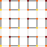
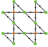
Figure 1: Left: A real space picture of a square lattice in the presence of a CDW and BDW in both $x$ and $y$ directions. Darker points indicate a higher electron density and darker lines an increased hopping between neighboring sites. Right: A real space picture of the CuO₂ plane showing the $\Theta_{2}$ planar loop order phase which produces a finite shear conductivity. Orange circles represent copper sites, green circles are oxygen sites, and arrows indicate the direction of spontaneously formed microscopic current loops.

A model calculation can be done by considering the most general Hamiltonian which includes charge and bond density waves (CDWs and BDWs) in both $x$- and $y$- directions. This captures the essential mirror-symmetry breaking physics, and more complicated candidate states (e.g. $d$-wave charge order) can be constructed from this model. At mean field level, the density wave Hamiltonian we consider is given by

$$\delta\mathcal{H}_{\text{DW}} =\sum_{\textbf{{R}}_{i}}\biggl{[}\phi_{\textbf{{R}}_{i}}c_{\textbf{{R}}_{i}}^{\dagger}c_{\textbf{{R}}_{i}}+\sum_{\alpha=x,y}\bigl{(}\Delta_{\textbf{{R}}_{i}}^{\alpha}c_{\textbf{{R}}_{i}+\textbf{{a}}_{\alpha}}^{\dagger}c_{\textbf{{R}}_{i}}+\text{H.c.}\bigr{)}\biggr{]}$$ (4)

where $\phi_{\textbf{{R}}_{i}}=\phi_{x}\cos(\textbf{{Q}}_{x}\cdot\textbf{{R}}_{i})+\phi_{y}\cos(\textbf{{Q}}_{y}\cdot\textbf{{R}}_{i})$ describes the CDW and $\Delta_{\textbf{{R}}_{i}}^{x/y}=\Delta_{x/y}\cos(\textbf{{Q}}_{x/y}\cdot\textbf{{R}}_{i})$ the BDW. We omit the spin degrees of freedom which will only double the overall conductivity, and for simplicity we consider period two density waves, i.e. $|\bm{Q}_{x/y}|=\pi$ . With these choices, a candidate striped state has (say) finite $\phi_{x}$ and $\Delta_{x}$ but $\phi_{y}=\Delta_{y}=0$, while a state with both $s$- and $d$-wave charge order in both $x$ and $y$ directions has finite $\phi_{x}=\phi_{y}$, along with finite $\Delta_{x}=-\Delta_{y}$. With similar generalizations, any candidate commensurate charge order can be included in this model Hamiltonian, and while the specific choice of ordering period will affect the following symmetry considerations, we consider the above an appropriate minimal model to calculate the shear conductivity.

Before proceeding with a formal calculation, it is useful to anticipate our results using symmetry arguments. From the real space picture in Fig. 1 it is easy to see that the vertical mirror plane symmetries $\hat{\sigma}_{x}$, and $\hat{\sigma}_{y}$ are broken only when finite period 2 charge and bond DW fields in both $x$ and $y$ directions are present. Finally, the product $\hat{\sigma}_{x=y}*C_{4}$ is also a broken symmetry, since the state is not invariant under four-fold rotations. Thus, we only expect a non-vanishing shear conductance for this system if all charge and bond fields are finite. Moreover, because a mirror reflection is implemented by the change in sign of any of the order parameters above, and $\Gamma_{xx,xy}$ much change sign under vertical mirror plane reflections, we expect that the shear conductivity is in general an odd power of each order parameter. The lowest order contribution would therefore be linear in each order parameter, i.e. $\Gamma\propto\phi_{x}\phi_{y}\Delta_{x}\Delta_{y}$

To apply this analysis to the cuprate like systems, we use a single band effective next-nearest neighbor tight-binding dispersion $\epsilon_{\textbf{{k}}}=-2t[\cos(k_{x})+\cos(k_{y})]+4t^{\prime}\cos(k_{x})\cos(k_{y})-\mu$ of the Cu square lattice with parameters $t^{\prime}=0.45t$ and $\mu=-0.65t$ (where $t$ is the nearest neighbor hopping for the unstrained system). The shear strain does not affect the nearest-neighbor hopping at $\mathcal{O}(\epsilon_{xy})$, but does modify the next nearest neighbor hopping. On the other hand, both the charge and the bond orders are unaffected at this order in strain. Rewriting the Hamiltonian in the four band basis of the new (four site) unit cell, and expanding Eq. (3) to linear order $\epsilon_{xy}$ in the limit $T\to 0$ then leads to $\sigma_{xx}^{\text{s}}=\sigma_{xx}+\Gamma_{xx,xy}\epsilon_{xy}=P_{x}+2P_{y}\epsilon_{xy}$ with

$$P_{\alpha}=\pi e^{2}\int\limits_{-\pi/2a}^{\pi/2a}\frac{d^{2}\textbf{{p}}}{(2\pi)^{2}}\,\mathbf{Re}\,\text{tr}\biggl{[}\hat{A}_{\textbf{{p}}}(0)\frac{\partial\hat{H}_{\textbf{{p}}}}{\partial p_{x}}\hat{A}_{\textbf{{p}}}(0)\frac{\partial\hat{H}_{\textbf{{p}}}}{\partial p_{\alpha}}\biggr{]}\,,$$ (5)

where the momentum integral is over the new reduced Brillouin zone. The results of the calculation are shown in Fig. 2, where we plot the ratio $\Gamma_{xx,xy}/\sigma_{xx}$ as a function of the charge order $\phi_{x}$ and $\Delta_{x}$. Consistent with our expectations based on symmetry, the response vanishes when any of $\phi_{x},\phi_{y},\Delta_{x}$, or $\Delta_{y}$ vanishes, since mirror symmetries are partially restored when this happens. Close to the onset temperature of such charge order, we expect the response to be small, as it is proportional to a high power of the order parameter fields. However, there is no reason to expect a small response well below the onset temperature, where the order parameters strengths are generically of order unity, in the case of long-range charge order.

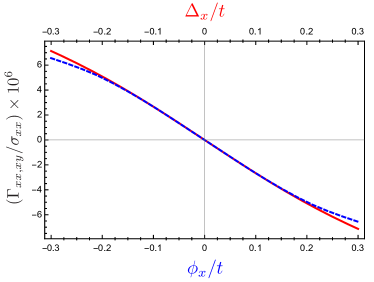
Figure 2: Ratio $\Gamma_{xx,xy}/\sigma_{xx}$ of shear conductivity over longitudinal conductivity for checkerboard charge and bond order (scattering time $\tau_{\text{sc}}=10/t$). Blue dashed curve as a function of $\phi_{x}$ for a finite and fixed value of the other three order parameters: $\phi_{y}=\Delta_{x}=-\Delta_{y}=0.1\,t$ and red curve as a function of $\Delta_{x}$ for similarly fixed $\phi_{x}=\phi_{y}=-\Delta_{y}=0.1\,t$.

III.3 Shear conductivity as a probe of loop current order

While it is now clear that charge ordered states exist within the pseudogap regime in many cuprates, a more vexing issue is the nature of the pseudogap itself. The pseudogap onset temperature $T^{*}$ is typically higher than the charge ordering temperature, with a primary experimental signature being the suppression of the electronic density of states NMRYBCO ; gurvitch1987resistivity ; Ding1996Spectroscopic ; timusk1999pseudogap , and the onset of $\bm{Q}=0$ magnetismBourges2006 ; Greven2008 ; Greven2010 . Such magnetic order is consistent with predictions first made by VarmaVarma99Pseudogap ; Varma2006 , who argued that various loop current states are responsible for the pseudogap phenomenology. Recent theoretical workTewari2008 ; aji2013magnetochiral ; yakovenko2015tilted ; varma2014gyrotropic has suggested that orbital current phases could also explain magneto-optic effects observed in the pseudogap regimeKerrYBCO ; Armitage . Here we discuss how planar versions of such a phase can be detected via shear conductivity measurements.

We have considered the so called $\Theta_{1}$ and $\Theta_{2}$ planar loop current states described in Ref. Varma2006, . As Fig. 1 demonstrates, the $\Theta_{2}$ state breaks all the required symmetries ($\hat{\sigma}_{x},\hat{\sigma}_{y},\hat{\sigma}_{(x=y)}*C_{4}$) to produce a shear conductivity, while the related $\Theta_{1}$ state with currents on all four diagonal bonds preserves the mirror planes $\hat{\sigma}_{x}$ and $\hat{\sigma}_{y}$ and so should not produce a shear conductivity response.

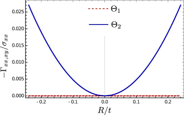
Figure 3: Ratio $\Gamma_{xx,xy}/\sigma_{xx}$ for the loop current states $\Theta_{1}$ (brown dashes) and $\Theta_{2}$ (blue) as function of the order parameter magnitudes $R/t$, where $t$ the tight-binding hopping parameter of the copper-oxygen bond. The response is parametrically larger than for charge order since it is quadratic in the magnitude of the small, dimensionless order parameters, $R/t$, and not quartic as in the case of charge order.

For a formal calculation, we work with a three band model that includes the Cu $d$-orbitals as well as the oxygen $p_{x}$- and $p_{y}$-orbitals and consider the mean-field Hamiltonian with order parameter $R$ of the loop current (formally an anapole or toroidal moment, which is a polar vector Rshekhter2009considerations ). Following the same procedure as before, we implement strain into this model by modifying the tight binding parameters and shearing the Brillouin zone. The results are shown in Fig. 3 and, as expected, the system shows a finite shear conductivity $\Gamma_{xx,xy}$ in the symmetry broken state $\Theta_{2}$, but not in $\Theta_{1}$.

We note that unlike the response to charge order, $\Gamma_{xx,xy}$ is even in the current loop order parameter, R. This follows from the symmetry of the $\Theta_{2}$ state, where the state with order parameter R is related to its time reversed partner by a $C_{2}$ rotation about the $z$ axis (see Fig. 1). Because a $C_{2}$ rotation leaves the tensor $\Gamma_{xx,xy}$ invariant, we have the equality $\Gamma_{xx,xy}(\textbf{{R}})=\Gamma_{xx,xy}(-\textbf{{R}})$. Therefore, the response must be proportional to an even power of R. We stress that the shear conductivity is likely to be considerably larger in the Varma current loop phase than in the charge ordered states studied in the previous section since it is proportional to a smaller power of the order parameter $R$ near the onset temperature, where a Landau-Ginzburg treatment remains valid.

IV Training the shear conductivity response

Having demonstrated that $\Gamma_{xx,xy}$ is finite when the requisite point group symmetries are broken, it is natural to ask whether the shear conductivity is measurable in macroscopic crystals where domains are inevitably present. Indeed, for both the charge and loop current order parameters, the response from different domains will cancel, as we discuss below. Nevertheless, because the response involves a product of order parameters (i.e. it is proportional to a composite order parameter), it is in fact possible to train this composite order parameter (and hence the shear conductivity) across the putative phase transition into a mirror symmetry breaking phase.

One can anticipate how such training is achieved based on general symmetry considerations: in crystals where a $D_{4h}$ point group symmetry is present in the symmetric phase (the corresponding space group is $P4/mmm)$, $\Gamma_{xx,xy}$ behaves like the $B_{2g}$ ($d_{xy}$) representation of $D_{4h}$, and so must be proportional to a composite order parameter with this symmetry. We can therefore train domains of such a composite order parameter by applying a shear strain, $\epsilon_{xy}$, through a symmetry breaking transition. Below, we discuss the formal symmetry considerations that allow such training for the loop current phase (where the absence of translation symmetry breaking makes the analysis simpler), and then the charge ordered phase.

First, in the case of the $\Theta_{2}$ loop current state, there are four possible domains: two time reversed partners with currents on the $x=y$ diagonals (with order parameters denoted as $\pm\textbf{{R}}^{a}$), and another two with currents on the opposite diagonal ($\pm\textbf{{R}}^{b}$). The responses from domains with currents on opposite diagonals cancel, because they are related by a $C_{4}$ rotation which sends $\Gamma_{xx,xy}(\textbf{{R}}^{a})\rightarrow-\Gamma_{yy,yx}(\textbf{{R}}^{b})=-\Gamma_{xx,xy}(\textbf{{R}}^{b})$, where the second equality follows from $\hat{\sigma}_{(x=y)}$ mirror symmetry of the state (see Appendix A.2). Nevertheless, because the responses from time reversed partners on a given diagonal are equal, a macroscopic response is possible if we can bias domains to be of a single orientation. This is easily accomplished by cooling through the loop current transition in the presence of an externally applied $B_{2g}$ strain field (a shear strain $\epsilon_{xy}$), which couples to the orientational component of the loop current order in the free energy like $\delta F=\lambda\epsilon_{xy}\left(|\textbf{{R}}^{a}|^{2}-|\textbf{{R}}^{b}|^{2}\right)$ where $\lambda$ is a coupling constant.

Next, in the case of the charge order considered in Sec. III.2, there are two possible domains of the composite order parameter $\phi_{x}\phi_{y}\Delta_{x}\Delta_{y}$, which if both present will lead to a vanishing shear conductivity. Nevertheless, while these individual order parameters cannot be trained, their product preserves translation symmetry while only breaking point group symmetries and so can once more be trained by application of an appropriate strain. We can determine the appropriate symmetry channel as follows: the composite order parameter $\phi_{x}\Delta_{x}$ is translation invariant for the case of $\bm{Q}_{x}=(\pi,0)$. This pattern breaks the $\hat{\sigma}_{x}$ mirror symmetry, and upon $C_{4}$ rotations, is transformed into the composite order parameter $\phi_{y}\Delta_{y}$. Thus, $\phi_{x}\Delta_{x}$ and $\phi_{y}\Delta_{y}$ have $p_{x}$ and $p_{y}$ symmetry, and so transform like components of the two dimensional $E_{u}$ representation of $D_{4h}$. The product of these two order parameters is therefore in the $B_{2g}$ representation of $D_{4h}$, and there is an allowed coupling to shear strain in the free energy, with a term of the form $\delta F=\lambda\epsilon_{xy}\phi_{x}\phi_{y}\Delta_{x}\Delta_{y}$. Applying shear strain and cooling through the charge ordering transition should therefore induce a finite shear conductivity response.

V Shear resistance measurements

Having computed $\Gamma_{xx,xy}$ for various ordered phases, we now discuss the experimental protocols required to measure such a response. Here, we build on recently used experimental methodsKuo1 ; Kuo2 ; Chu12 for determining specific terms in the elastoresistivity tensor $m_{\alpha\beta,\gamma\delta}=\frac{\partial\left[\left(\nicefrac{{\Delta\rho}}{{\rho}}\right)_{\alpha\beta}\right]}{\partial\epsilon_{\gamma\delta}}\bigr{|}_{\epsilon\rightarrow 0}$ which describes the strain-induced change in the normalized resistivity. The technique, which was originally employed to reveal the presence of nematic fluctuations, can be generalized in the following way.

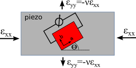
Figure 4: Experimental setup for the detection of shear resistance similar to Ref. [Kuo1, ; Kuo2, ]

A rectangular sample with principal axes $a,b$ oriented along its edges is glued with a relative angle $\theta$ onto a piezoelectric stack in order to measure the longitudinal elastoresistance (Fig. 4). Applying a voltage to the piezo leads to a stress and therefore tensile strains $\epsilon_{xx}$ and $\epsilon_{yy}=-\nu_{p}\epsilon_{xx}$ (where $\nu_{p}$ is the Poisson ratio of the piezoelectric stack) in the coordinate system of the piezo stack. Since the sample is mounted with a relative angle on the piezo element, the pure tensile strain of the piezo stack translates into a combination of tensile and shear strain in the coordinate system of the crystal axes $a,b$ for the sample.

Measuring the change of the resistance $\left(\nicefrac{{\Delta R}}{{R}}\right)_{xx}\simeq\left(\nicefrac{{\Delta\rho}}{{\rho}}\right)_{xx}$ due to the applied strain for several angles $\theta$, the angularly antisymmetric component of the response is given by

$$\left(\frac{\Delta R}{R}\right)^{\text{odd}}_{xx}\kern-10.00002pt(\theta) =\frac{1}{2}\left[\left(\frac{\Delta R}{R}\right)_{xx}\kern-10.00002pt(\theta)-\left(\frac{\Delta R}{R}\right)_{xx}\kern-10.00002pt(-\theta)\right]$$ (6)

$$=(\nu_{p}+1)\,\biggl{[}\frac{m_{xx,zz}C_{zz,xy}}{C_{zz,zz}}-m_{xx,xy}\biggr{]}\sin(2\theta)\cdot\epsilon_{xx},$$

where $C_{ij,kl}$ are components of the elastic stiffness tensor. For tetragonal or orthorhombic symmetry, $C_{zz,xy}=m_{xx,xy}=0$, and the odd contribution vanishes; conversely, a nonzero $\left(\nicefrac{{\Delta R}}{{R}}\right)^{\text{odd}}_{xx}$ is proof of broken mirror symmetries. An equivalent approach involves using lithographic methods to prepare samples with different axes orientations (see Appendix E).

VI Discussion

We have demonstrated the use of a higher rank tensor — the shear conductivity $\Gamma_{xx,xy}$ — as a sensitive probe of broken point group symmetries. In the context of the cuprates, the onset of such a response at the charge ordering temperature would unambiguously demonstrate that charge order breaks all in-plane mirror reflection symmetries; recall these are discrete symmetries which are less susceptible to disorder and can survive as true long range ordered states. However, it is possible that a current loop state onsets at a higher, pseudogap temperature scale, in which case the detection of $\Gamma_{xx,xy}$ at $T^{*}$ supports proposals of the $\Theta_{2}$ version of this $\bm{Q}=0$ magnetic state. In either scenario, any identification of broken mirror symmetries is significant as it specifies a true thermodynamic phase in the pseudogap regime, and places constraints on a putative quantum critical point which may exist near optimal doping in cuprate materials.

To summarize, we have considered transport coefficients in the presence of strain that are direct indicators of mirror symmetry breaking. We have studied the shear conductivity in the context of two broken symmetry phases that have been proposed to occur within the pseudogap regime of hole-doped cuprates and have discussed experimental protocols to measure such response. Our analysis can be generalized to study other components of the strain conductivity tensor $\Gamma_{ijkl}$.

VII Acknowledgements

We thank A.T. Hristov and Chandra Varma for useful discussions. SR would also like to thank the KITP-UCSB Research Program, Magnetism, Bad Metals and Superconductivity , for hospitality. PH was supported with a PhD-fellowship of the Deutscher Akademischer Austauschdienst (DAAD). Work at Stanford University was supported by the Department of Energy, Office of Basic Energy Sciences under contract DE-AC02-76SF00515 (AM, PH, MS, SR and IF), and the Alfred P. Sloan Foundation (SR).

Appendix A Symmetry considerations

A.1 General properties of tensorial response functions

Given a Hamiltonian $\mathcal{H}$ that is invariant under the point group transformation $\hat{O}:\textbf{{r}}\rightarrow\textbf{{r}}^{\prime}$, a physical response function $R_{x_{1},\ldots,x_{n}}$, which is a tensor of rank $n$ (e.g. resistivity, elasticity, etc.) is constrained according to

$$R_{x_{1},\ldots,x_{n}} =\hat{O}_{x_{1},y_{1}}\ldots\hat{O}_{x_{n},y_{n}}R_{y_{1},\ldots y_{n}}.$$ (7)

This condition typically restricts several elements of $\hat{R}$ to vanish; conversely, breaking some point group symmetries relaxes these constraints, allowing the new responses to serve as evidence of broken symmetry. In the following, we will restrict ourselves to the case of (quasi) two-dimensional materials as the various cuprates, iron-based superconductors or heavy-fermion compounds mostly possess a tetragonal symmetry in the high-temperature regime. Nevertheless, it is straightforward to generalize these considerations to more general crystal classes.

Consider now a state that is invariant under reflection about say the $xy$-plane ($\hat{\sigma}_{z}:\{x,y,z\}\rightarrow\{x,y,-z\}$). We find the condition that

$$R_{x_{1},\ldots,x_{n}}=(-1)^{N_{z}}R_{x_{1},\ldots,x_{n}}$$

, where $N_{z}$ is the number of $z$-indices (and likewise for $\hat{\sigma}_{x}$ and $\hat{\sigma}_{y}$ symmetry). Fourfold rotation symmetry about the $z$-axis leads to the conditions

$$R_{x_{1},\ldots,x_{n}}=(-1)^{N_{x}}R_{x_{1},\ldots,x_{n}}\bigr{|}_{x\leftrightarrow y},$$

and

$$R_{x_{1},\ldots,x_{n}}=(-1)^{N_{y}}R_{x_{1},\ldots,x_{n}}\bigr{|}_{x\leftrightarrow y}.$$

Finally, a mirror symmetry $\hat{\sigma}_{(x=y)}$ (about the $(x=-y)z$ plane) implies the condition

$$R_{x_{1},\ldots,x_{n}}=R_{x_{1},\ldots,x_{n}}\bigr{|}_{x\leftrightarrow y}.$$

Of particular interest to us is the shear conductivity component $\Gamma_{xx,xy}=\partial\sigma_{xx}/\partial\epsilon_{xy}$ for 2D systems, which describes the change of the longitudinal DC conductivity induced by a shear strain of the crystal. Based on the above symmetry considerations, this can be non-vanishing only when reflections about the $x$- and the $y$-axes – $\hat{\sigma}_{y}$, $\hat{\sigma}_{x}$ – as well as the combination $\hat{\sigma}_{(x=y)}*C_{4}$, where $\hat{\sigma}_{(x=y)}$ denotes reflection about the vertical $(x=-y)z$ plane and $C_{4}$ a $\pi/2$ rotation about the $z$-axis, are broken. Following these lines, it is straightforward to construct the explicit forms of higher-rank tensors as the elastoresistance or the elastic stiffness systems with arbitrary symmetries, see e.g., Section E.

A.2 Properties of $\Gamma_{xx,xy}$ for planar loop currents

We now discuss properties of the shear conductivity within a given loop current state, i.e. a single domain which corresponds to one configuration of the loop current order parameter R. The magnetic point group symmetry within the loop current state is isomorphic to $D_{2h}$shekhter2009considerations , with the following group elements in addition to the identity: $C_{2}(z)\mathcal{T}$, $C_{2}(x=y)\mathcal{T}$, $C_{2}(x=-y)$, $i\mathcal{T}$, $\hat{\sigma}_{z}$, $\hat{\sigma}_{(x=-y)}\mathcal{T}$, and $\hat{\sigma}_{(x=y)}$, where $C_{2}(z)$ denotes a 180 degree rotation about the $z$ axis etc., $\mathcal{T}$ denotes time reversal, $i$ is inversion, and $\hat{\sigma}_{(x=y)}$ denotes mirror reflection as before etc. Note that these are the group elements for the configuration shown in Fig. 1. These group operations place the following constraints on the shear conductivity in the presence of a $c$ axis directed magnetic field, $H_{z}$:

$$C_{2}(z)\mathcal{T},\,i\mathcal{T}:\quad\Gamma_{xx,xy}(\textbf{{R}},H_{z}) =\Gamma_{xx,xy}(\textbf{{R}},-H_{z})$$ (8)

$$C_{2}(x=-y),\hat{\sigma}_{(x=y)}:\quad\Gamma_{xx,xy}(\textbf{{R}},H_{z}) =\Gamma_{yy,yx}(\textbf{{R}},-H_{z})$$ (9)

$$C_{2}(x=y)\mathcal{T},\hat{\sigma}_{(x=-y)}\mathcal{T}:\quad\Gamma_{xx,xy}(\textbf{{R}},H_{z}) =\Gamma_{yy,yx}(\textbf{{R}},H_{z}).$$ (10)

while $\hat{\sigma}_{z}$ places no constraint. For clarity, note that $C_{2}\mathcal{T}$ and $i\mathcal{T}$ independently imply the identity of Eq. 8, and similarly for the subsequent equations.

A.3 Properties of $\Gamma_{xx,xy}$ for charge order

In the case of the charge order described in Sec. III.2, the point group symmetry is much more restricted. In the case of equal magnitude charge and bond order parameters as drawn in Fig. 1, with $|\phi_{x}|=|\phi_{y}|$ and $|\Delta_{x}|=|\Delta_{y}|$, the point group symmetry is $C_{2v}$, with the group elements $C_{2}(x=-y)$, $\hat{\sigma}_{(x=y)}$, and $\hat{\sigma}_{z}$ in addition to the identity. These enforce the following constraints on the shear conductivity in a $c$ axis directed magnetic field:

$$C_{2}(x=-y),\hat{\sigma}_{(x=y)}:\quad\Gamma_{xx,xy}(H_{z}) =\Gamma_{yy,yx}(-H_{z})$$ (11)

while $\hat{\sigma}_{z}$ places no constraint. Alternatively, when the magnitudes of the order parameters are different, with $|\phi_{x}|\neq|\phi_{y}|$ and $|\Delta_{x}|\neq|\Delta_{y}|$ the point group symmetry is reduced to $C_{s}$, with only two group elements: the identity, and $\hat{\sigma}_{x=y}$. This places no constrains on transformations of $\Gamma_{xx,xy}$.

Appendix B Linear Response theory of elastoconductivity

In this section we derive the general expression for the elastoconductivity using Kubo’s Linear Response theory. The presented formalism is suitable for any kind of bilinear Hamiltonian with the form

$$\mathcal{H}=\sum_{\textbf{{k}},\alpha\beta}H_{\textbf{{k}},\alpha\beta}c_{\textbf{{k}},\alpha}^{\dagger}c_{\textbf{{k}},\beta}=\sum_{\textbf{{k}}}\hat{\Psi}_{\textbf{{k}}}^{\dagger}\hat{H}_{\textbf{{k}}}\hat{\Psi}_{\textbf{{k}}},$$ (12)

with corresponding Matsubara Green’s function $\hat{G}_{\textbf{{k}}}(i\omega_{n})=\bigl{[}i\omega_{n}\mathds{1}-\hat{H}_{\textbf{{k}}}\bigr{]}^{-1}$. Following Mahan mahan2000many the longitudinal DC conductivity for such a multiband system can be calculated to be

$$\sigma_{xx}=-\pi e^{2}\int\limits_{\text{1st B.Z.}}\frac{d^{d}\textbf{{k}}}{(2\pi)^{d}}\int\limits_{-\infty}^{\infty}d\epsilon\frac{\partial f(\epsilon)}{\partial\epsilon}\mathbf{Re}\,\text{tr}\biggl{[}\bigl{(}\hat{A}_{\textbf{{k}}}(\epsilon)\frac{\partial\hat{H}_{\textbf{{k}}}}{\partial k_{x}}\bigr{)}^{2}\biggr{]},$$ (13)

where $\hat{A}_{\textbf{{k}}}(\epsilon)=\frac{i}{2\pi}\bigl{[}\hat{G}_{\textbf{{k}}}(\epsilon+i/2\tau_{\text{sc}})-\hat{G}_{\textbf{{k}}}(\epsilon-i/2\tau_{\text{sc}})\bigr{]}$ is the spectral weight of the system, $\epsilon$ is an energy and $f(\epsilon)$ is the usual Fermi-Dirac distribution function. In order to yield a finite result of this transport expression, it is necessary to introduce a finite lifetime $\tau_{\text{sc}}$ for the fermionic quasiparticles, which can originate from electron-electron, electron-phonon or electron-impurity interactions. Here, we just assume $\tau_{\text{sc}}\neq 0$, and neglect other processes (e.g., vertex corrections). Thus, the scattering rate $1/\tau_{\text{sc}}\ll E_{F}$ (where $E_{F}$ is the Fermi energy) can be viewed simply as an effective parameter of the theory.

We now focus on two spatial dimensions and consider a system with a Hamiltonian (12), to be described by a tight-binding model

$$\mathcal{H} =\sum_{\textbf{{R}}_{i}}\sum_{\alpha,\beta}\epsilon^{\alpha\beta}c_{i,\alpha}^{\dagger}c_{i,\beta}+\sum_{<\textbf{{R}}_{i},\textbf{{R}}_{j}>}\sum_{\alpha,\beta}\bigl{[}t_{ij}^{\alpha\beta}c_{i,\alpha}^{\dagger}c_{j,\beta}+\text{h.c.}\bigr{]}+\sum_{<<\textbf{{R}}_{i},\textbf{{R}}_{j}>>}\sum_{\alpha,\beta}\bigl{[}(t^{\prime})_{ij}^{\alpha\beta}c_{i,\alpha}^{\dagger}c_{j,\beta}+\text{h.c.}\bigr{]}+\ldots,$$ (14)

where $\textbf{{R}}_{i}$ are the positions of the atoms of the lattice (Bravais vectors $\textbf{{a}}_{1},\textbf{{a}}_{2}$) and $\alpha$ describes for example possible orbital or spin degrees of freedom. The matrix/hopping elements $(t^{n})_{ij}^{\alpha\beta}$ are in general dependent on the distance between the atoms, which can be parameterized as

$$(t^{n})_{ij}^{\alpha,\beta}=\bigr{[}t^{n}(|\textbf{{R}}_{i}-\textbf{{R}}_{j}|)\bigr{]}^{\alpha\beta}=(t^{n})^{\alpha\beta}e^{-\gamma_{n}^{\alpha\beta}\bigl{[}|\textbf{{R}}_{i}-\textbf{{R}}_{j}|-|\textbf{{R}}_{i}^{0}-\textbf{{R}}_{j}^{0}|\bigr{]}},$$ (15)

where $\textbf{{R}}_{i}^{0}$ are the equilibrium positions of the atoms. Without strain, the Fourier space representation of (14) is just given by

$$\mathcal{H} =\sum_{\textbf{{k}}}\sum_{\alpha,\beta}c_{\textbf{{k}},\alpha}^{\dagger}c_{\textbf{{k}},\beta}\biggl{[}\epsilon^{\alpha\beta}+2t^{\alpha\beta}\bigl{[}\cos(\textbf{{a}}_{1}\cdot\textbf{{k}})+\cos(\textbf{{a}}_{2}\cdot\textbf{{k}})\bigr{]}$$

$$\hskip 8.5359pt+2(t^{\prime})^{\alpha\beta}\bigl{[}\cos([\textbf{{a}}_{1}+\textbf{{a}}_{2}]\cdot\textbf{{k}})+\cos([\textbf{{a}}_{1}-\textbf{{a}}_{2}]\cdot\textbf{{k}})\bigr{]}+\ldots\biggr{]}$$

$$=\sum_{\textbf{{k}}}\Psi_{\textbf{{k}}}^{\dagger}\hat{H}_{\textbf{{k}}}\Psi_{\textbf{{k}}},$$ (16)

with the spinor $\Psi_{k}=(c_{k,1},c_{k,2},\ldots)^{T}$ describing the multiband system. We now apply a general strain to the crystal, which has the form

$$\hat{\epsilon}=\left(\begin{matrix}\epsilon_{xx}&\epsilon_{xy}\\ \epsilon_{xy}&\epsilon_{yy}\end{matrix}\right).$$ (17)

The strain changes the Bravais lattice vectors $\textbf{{a}}_{1},\textbf{{a}}_{2}$ of the system to

$$\textbf{{a}}_{j}^{\text{s}}=(\hat{\mathds{1}}+\hat{\epsilon})\textbf{{a}}_{j},\quad j=1,2$$ (18)

and therefore also the positions of the atoms $\textbf{{R}}_{i}^{0}\rightarrow\textbf{{R}}_{i}^{\text{s}}=(\hat{\mathds{1}}+\hat{\epsilon})\textbf{{R}}_{i}$. The Hamiltonian in the presence of strain is therefore given by

$$\mathcal{H}^{\text{s}} =\sum_{\textbf{{k}}}{}^{\prime}\sum_{\alpha,\beta}c_{\textbf{{k}},\alpha}^{\dagger}c_{\textbf{{k}},\beta}\biggl{[}\epsilon^{\alpha\beta}+2t^{\alpha\beta}\sum_{j=1,2}e^{-\gamma^{\alpha\beta}\bigl{[}|(\hat{\mathds{1}}+\hat{\epsilon})\textbf{{a}}_{j}|-|\textbf{{a}}_{j}|\bigr{]}}\cos([(\hat{\mathds{1}}+\hat{\epsilon})\textbf{{a}}_{j}]\cdot\textbf{{k}})$$

$$\hskip 76.82234pt+2(t^{\prime})^{\alpha\beta}\sum_{j=\pm}e^{-\gamma^{\prime\alpha\beta}\bigl{[}|(\hat{\mathds{1}}+\hat{\epsilon})(\textbf{{a}}_{1}+j\textbf{{a}}_{2})|-|\textbf{{a}}_{1}+j\textbf{{a}}_{2}|\bigr{]}}\cos([(\hat{\mathds{1}}+\hat{\epsilon})(\textbf{{a}}_{1}+j\textbf{{a}}_{2})]\cdot\textbf{{k}})+\ldots\biggr{]}$$

$$=\sum_{\textbf{{k}}}{}^{\prime}\,\Psi_{\textbf{{k}}}^{\dagger}\hat{H}_{(\hat{\mathds{1}}+\hat{\epsilon})\textbf{{k}}}^{\text{s}}\Psi_{\textbf{{k}}}.$$ (19)

Note that there are now three major changes if we compare (19) with (16): i) Due to (18), the Brillouin zone is strained, which is indicated by $\sum_{\textbf{{k}}}{}^{\prime}$; ii) the Hamiltonian matrix

$$\hat{H}_{(\hat{\mathds{1}}+\hat{\epsilon})\textbf{{k}}}^{\text{s}}=\hat{H}_{(\hat{\mathds{1}}+\hat{\epsilon})\textbf{{k}}}\biggr{|}_{(t^{n})_{ij}^{\alpha\beta}\rightarrow(t^{n})_{ij}^{\alpha\beta}(\hat{\epsilon})},$$ (20)

has modified tight-binding parameters depending on the strain $\hat{\epsilon}$; and iii) the quasimomentum $\textbf{{k}}\rightarrow(\hat{\mathds{1}}+\hat{\epsilon})\textbf{{k}}$ takes into account the change of the Brillouin zone. Inserting now our strained Hamiltonian (19) into the linear response theory we find

$$\sigma_{xx}^{\text{s}} =-\pi e^{2}\int\limits_{\text{strained}\atop\text{1st B.Z.}}\frac{d^{2}\textbf{{k}}}{(2\pi)^{2}}\int\limits_{-\infty}^{\infty}d\epsilon\frac{\partial f(\epsilon)}{\partial\epsilon}\mathbf{Re}\,\text{tr}\biggl{[}\biggl{(}\hat{A}_{(\hat{\mathds{1}}+\hat{\epsilon})\textbf{{k}}}^{\text{s}}(\epsilon)\frac{\partial\hat{H}_{(\hat{\mathds{1}}+\hat{\epsilon})\textbf{{k}}}^{\text{s}}}{\partial k_{x}}\biggr{)}^{2}\biggr{]}$$

$$=-\frac{\pi e^{2}}{\text{det}(\hat{\mathds{1}}+\hat{\epsilon})}\int\limits_{\text{1st B.Z.}}\frac{d^{2}\textbf{{p}}}{(2\pi)^{2}}\int\limits_{-\infty}^{\infty}d\epsilon\frac{\partial f(\epsilon)}{\partial\epsilon}\mathbf{Re}\,\text{tr}\biggl{[}\biggl{(}\hat{A}_{\textbf{{p}}}^{\text{s}}(\epsilon)\bigl{[}(1+\epsilon_{xx})\frac{\partial\hat{H}_{\textbf{{p}}}^{s}}{\partial p_{x}}+\epsilon_{xy}\frac{\partial\hat{H}_{\textbf{{p}}}^{s}}{\partial p_{y}}\bigr{]}\biggr{)}^{2}\biggr{]},$$ (21)

where in the second line we substituted $\textbf{{p}}=(\hat{\mathds{1}}+\hat{\epsilon})\textbf{{k}}$ so that the integral over the original (unstrained) Brillouin zone is recovered. In the following we will always differentiate between the momentum k defined in the strained Brillouin zone and p in the unstrained Brillouin zone (see Fig. 5).

Figure 5: Unstrained and sheared Bravais lattice and corresponding first Brillouin zone of square lattices.

B.1 Next-nearest neighbor tight-binding dispersion for square lattice in the presence of shear strain

In order to make the connection between the generalized tight-binding Hamiltonian in (16) to the systems considered in this paper, we now calculate the dispersion of a simple square lattice in next-nearest neighbor approximation and in the presence of a pure shear strain

$$\hat{\epsilon}=\left(\begin{matrix}0&\epsilon_{xy}\\ \epsilon_{xy}&0\end{matrix}\right)\,.$$ (22)

The Bravais vectors of a square lattice are $\textbf{{a}}_{1}=\textbf{{e}}_{x},\textbf{{a}}_{2}=\textbf{{e}}_{y}$, where we set the lattice constant $a=1$. The nearest-neighbor hoppings $t^{\text{s}}=t$ (and also the charge and bond order parameters) do not change linearly in $\epsilon_{xy}$ by a pure shear strain since the distance between neighbor atoms is $|(\hat{\mathds{1}}+\hat{\epsilon})\textbf{{e}}_{x/y}|=1+\frac{1}{2}\epsilon_{xy}^{2}\approx 1$. In contrast, the next-nearest neighbor hoppings

$$\bigl{[}t^{\prime}(\textbf{{e}}_{x}^{\text{s}}\pm\textbf{{e}}_{y}^{\text{s}})\bigr{]}^{\text{s}}=t^{\prime}e^{-\gamma^{\prime}\bigl{(}|\textbf{{e}}_{x}^{\text{s}}\pm\textbf{{e}}_{y}^{\text{s}}|-|\textbf{{e}}_{x}\pm\textbf{{e}}_{y}|\bigr{)}}\approx t^{\prime}\bigl{(}1\mp\sqrt{2}\gamma^{\prime}\epsilon_{xy}\bigr{)},$$ (23)

obtain a linear $\epsilon_{xy}$-dependence and we get the sheared dispersion

$$\epsilon_{\textbf{{p}}}^{\text{s}} =2t\bigl{[}\cos(p_{x})+\cos(p_{y})\bigr{]}+2t^{\prime}\bigl{(}1-\sqrt{2}\gamma^{\prime}\epsilon_{xy}\bigr{)}\cos(p_{x}+p_{y})$$

$$\qquad+2t^{\prime}\bigl{(}1+\sqrt{2}\gamma^{\prime}\epsilon_{xy}\bigr{)}\cos(p_{x}-p_{y})-\mu.$$ (24)

Note that p is, as mentioned in the last section, the momentum in the unstrained Brillouin zone which has to be used in formula (21).

Appendix C Shear conductivity in cuprates with charge order

C.1 Effective Hamiltonian for bidirectional charge order

A bidirectional charge ($\phi$) and bond ($\Delta$) density wave of period $N\in\mathbb{N}$ on a square lattice (which describes our quasi two-dimensional material) is described by the commensurate fields

$$\begin{split}\phi_{\textbf{{R}}_{i}}&=\phi_{x}\cdot\cos(\textbf{{Q}}_{x}\cdot\textbf{{R}}_{i})+\phi_{y}\cdot\cos(\textbf{{Q}}_{y}\cdot\textbf{{R}}_{i}),\\ \Delta^{x/y}_{\textbf{{R}}_{i}}&=\Delta_{x/y}\cdot\cos(\textbf{{Q}}_{x/y}\cdot\textbf{{R}}_{i}),\end{split}$$ (25)

where $\phi_{x/y},\Delta_{x/y}\in\mathbb{R}$ and $\textbf{{Q}}_{x/y}=\frac{2\pi}{N}\textbf{{e}}_{x/y}$. Note that $C_{4}$ symmetric (i.e., “checkerboard”) order with $\phi_{x}=\phi_{y}$ and $\Delta_{x}=\Delta_{y}$, also preserves the $\hat{\sigma}_{(x=-y)}$ symmetry. We consider here the effective square copper lattice (Bravais lattice $\textbf{{a}}_{x}=\textbf{{e}}_{x},\textbf{{a}}_{y}=\textbf{{e}}_{y}$) describing the material’s dispersion (note that we have ignored spin degrees of freedom which simply contribute an overall factor of 2 in the conductivity). The effective Hamiltonian reads

$$\mathcal{H}=\sum_{\textbf{{R}}_{i}}\bigl{[}\phi_{\textbf{{R}}_{i}}-\mu\bigr{]}c_{i}^{\dagger}c_{i}+\biggl{[}-\sum_{\alpha=x,y}\sum_{\textbf{{R}}_{j}=\textbf{{R}}_{i}+\textbf{{a}}_{\alpha}}\bigl{[}t+\Delta^{\alpha}_{\textbf{{R}}_{i}}\bigr{]}c_{j}^{\dagger}c_{i}+t^{\prime}\sum_{\textbf{{R}}_{j}=\textbf{{R}}_{i}+\textbf{{a}}_{x}\pm\textbf{{a}}_{y}}c_{j}^{\dagger}c_{i}+\text{h.c.}\biggr{]},$$ (26)

where we use the parameters $t=1,t^{\prime}=0.45t,\mu=-0.65t$. Transforming this Hamiltonian into Fourier space leads to

$$\mathcal{H} =\sum_{\textbf{{k}}}\epsilon_{\textbf{{k}}}c_{\textbf{{k}}}^{\dagger}c_{\textbf{{k}}}+\sum_{\textbf{{k}}}\sum_{\alpha=x,y}\biggl{(}\biggl{[}\frac{\phi_{\alpha}}{2}-\Delta_{\alpha}e^{-i\textbf{{Q}}_{\alpha}\cdot\textbf{{a}}_{\alpha}}\cos\bigl{[}(\textbf{{k}}+\frac{\textbf{{Q}}_{\alpha}}{2})\cdot\textbf{{a}}_{\alpha}\bigr{]}\biggr{]}c_{\textbf{{k}}+\textbf{{Q}}_{\alpha}}^{\dagger}c_{\textbf{{k}}}+\text{h.c.}\biggr{)},$$ (27)

with the free dispersion

$$\epsilon_{\textbf{{k}}}=-2t[\cos(k_{x})+\cos(k_{y})]+4t^{\prime}\cos(k_{x})\cos(k_{y})-\mu.$$ (28)

Due to the density waves the periodicity of the crystal changes from $a=1$ to $N$, so we have downfolded our original Brillouin zone

$$k_{x/y}\in[-\pi,\pi]\quad\rightarrow\quad k_{x/y}\in[-\pi/N,\pi/N],$$ (29)

so that we end up with an effective band Hamiltonian

$$\mathcal{H} =\sum_{\textbf{{k}}}\Psi_{\textbf{{k}}}^{\dagger}\hat{H}_{\textbf{{k}}}\Psi_{\textbf{{k}}},$$ (30)

where $\Psi_{\textbf{{k}}}=(c_{\textbf{{k}}},c_{\textbf{{k}}+\textbf{{Q}}_{x}},\ldots)^{T}$. From this point on we will restrict ourselves to the case of $N=2$, but the following arguments and steps are valid for arbitrary $N$. For $N=2$ we have the spinor $\Psi_{\textbf{{k}}}=(c_{\textbf{{k}}},c_{\textbf{{k}}+\textbf{{Q}}_{x}},c_{\textbf{{k}}+\textbf{{Q}}_{y}},c_{\textbf{{k}}+\textbf{{Q}}_{x}+\textbf{{Q}}_{y}})^{T}$ and the Hamiltonian

$$\hat{H}_{\textbf{{k}}} =\left(\begin{matrix}\epsilon_{\textbf{{k}}}&\chi_{x}(\textbf{{k}})&\chi_{y}(\textbf{{k}})&0\\ \chi_{x}^{*}(\textbf{{k}})&\epsilon_{\textbf{{k}}+\textbf{{Q}}_{x}}&0&\chi_{y}(\textbf{{k}}+\textbf{{Q}}_{x})\\ \chi_{y}^{*}(\textbf{{k}})&0&\epsilon_{\textbf{{k}}+\textbf{{Q}}_{y}}&\chi_{x}(\textbf{{k}}+\textbf{{Q}}_{y})\\ 0&\chi_{y}^{*}(\textbf{{k}}+\textbf{{Q}}_{x})&\chi_{x}^{*}(\textbf{{k}}+\textbf{{Q}}_{y})&\epsilon_{\textbf{{k}}+\textbf{{Q}}_{x}+\textbf{{Q}}_{y}}\end{matrix}\right),$$ (31)

with

$$\chi_{x/y}(\textbf{{k}})=\phi_{x/y}+2\Delta_{x/y}e^{-i\textbf{{Q}}_{x/y}\cdot\textbf{{a}}_{x/y}}\cos\bigl{[}(\textbf{{k}}+\textbf{{Q}}_{x/y}/2)\cdot\textbf{{a}}_{x/y}\bigr{]}=\phi_{x/y}-2i\Delta_{x/y}\cos\bigl{[}k_{x/y}+\pi/2\bigr{]}.$$ (32)

In Fig. 6 we show the original cuprate Fermi surface and the down-folded Fermi surface for the period $2$ charge and bond density waves.

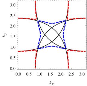
Figure 6: Fermi surface of the original (left) and down-folded (right) Brillouin zone for charge and bond order ($N=2$) with gaps opening at the hot spots of the Fermi surface that are connected by $\textbf{{Q}}_{x/y}=\pi\textbf{{e}}_{x/y}$. Note that the figure on the right is the reduced Brillouin zone shown here as the upper right corner of the original Brillouin zone.

C.2 Shear conductivity

We now discuss how to apply the shear strain (22) on the density wave system. The change of the Bravais-lattice $\textbf{{a}}_{x/y}^{\text{s}}=(\mathds{1}+\hat{\epsilon})\textbf{{a}}_{x/y}$ will also lead to a change of the reciprocal lattice vectors $\textbf{{b}}_{x/y}^{\text{s}}=\frac{2\pi}{V}(\textbf{{e}}_{z}\times\textbf{{a}}_{y/x}^{\text{s}})$ and finally also the ordering vector $\textbf{{Q}}_{x/y}^{\text{s}}=\frac{1}{N}\textbf{{b}}_{x/y}^{\text{s}}$. This means that

$$\textbf{{Q}}_{\alpha}\cdot\textbf{{a}}_{\beta}=\textbf{{Q}}_{\alpha}^{\text{s}}\cdot\textbf{{a}}_{\beta}^{\text{s}}=\frac{2\pi}{N},$$ (33)

remains invariant under the application of the strain. As we saw in Section B.1, the nearest neighbor hoppings are not affected linearly in $\epsilon_{xy}$ by a pure shear strain and the same argument should therefore hold for the charge and bond order $\phi_{x/y},\Delta_{x/y}$ since their ordering vectors are aligned with the $x$ and $y$ axis. This means that the strained Hamiltonian of (31) is given by

$$\hat{H}^{\text{s}}_{\textbf{{p}}} =\left(\begin{matrix}\epsilon^{\text{s}}_{\textbf{{p}}}&\chi_{x}(\textbf{{p}})&\chi_{y}(\textbf{{p}})&0\\ \chi_{x}^{*}(\textbf{{p}})&\epsilon^{\text{s}}_{\textbf{{p}}+\textbf{{Q}}_{x}}&0&\chi_{y}(\textbf{{p}}+\textbf{{Q}}_{x})\\ \chi_{y}^{*}(\textbf{{p}})&0&\epsilon^{\text{s}}_{\textbf{{p}}+\textbf{{Q}}_{y}}&\chi_{x}(\textbf{{p}}+\textbf{{Q}}_{y})\\ 0&\chi_{y}^{*}(\textbf{{p}}+\textbf{{Q}}_{x})&\chi_{x}^{*}(\textbf{{p}}+\textbf{{Q}}_{y})&\epsilon^{\text{s}}_{\textbf{{p}}+\textbf{{Q}}_{x}+\textbf{{Q}}_{y}},\end{matrix}\right)$$ (34)

with the strained dispersion $\epsilon^{\text{s}}_{\textbf{{p}}}$ defined in (24). We now rewrite the formula for the elastoconductivity in the case of pure shear strain

$$\sigma_{xx}^{\text{s}} \stackrel{{\scriptstyle(\ref{sa8})}}{{=}}-\frac{\pi e^{2}}{1-\epsilon_{xy}^{2}}\underbrace{\int\limits_{\text{1st B.Z.}}}_{\int_{-\pi/2}^{\pi/2}}\frac{d^{2}\textbf{{p}}}{(2\pi)^{2}}\int\limits_{-\infty}^{\infty}d\epsilon\frac{\partial f(\epsilon)}{\partial\epsilon}\mathbf{Re}\,\text{tr}\biggl{[}\bigl{(}\hat{A}_{\textbf{{p}}}^{\text{s}}(\epsilon)\hat{J}_{\textbf{{p}},x}^{\text{s}}\bigr{)}^{2}\biggr{]},$$ (35)

where the integral is performed over the reduced Brillouin zone and we have defined the current vertex as

$$\hat{J}_{\textbf{{p}},x}^{\text{s}}=\frac{\partial\hat{H}_{\textbf{{p}}}^{s}}{\partial p_{x}}+\epsilon_{xy}\frac{\partial\hat{H}_{\textbf{{p}}}^{s}}{\partial p_{y}}.$$ (36)

Expanding the spectral weight and the current operator to linear order in the shear strain $\epsilon_{xy}$ we have

$$\begin{split}\hat{A}_{\textbf{{p}}}^{\text{s}}(\epsilon)&=\hat{A}_{\textbf{{p}}}^{\text{s}}(\epsilon)\biggr{|}_{\epsilon_{xy}=0}+\frac{\hat{A}_{\textbf{{p}}}^{\text{s}}(\epsilon)}{\partial\epsilon_{xy}}\biggr{|}_{\epsilon_{xy}=0}\cdot\epsilon_{xy}=\hat{A}_{\textbf{{p}}}(\epsilon)+\delta\hat{A}_{\textbf{{p}}}(\epsilon)\cdot\epsilon_{xy}\\ \hat{J}_{\textbf{{p}},x}^{\text{s}}&=\hat{J}_{\textbf{{p}},x}^{\text{s}}\biggr{|}_{\epsilon_{xy}=0}+\frac{\hat{J}_{\textbf{{p}},x}^{\text{s}}}{\partial\epsilon_{xy}}\biggr{|}_{\epsilon_{xy}=0}\cdot\epsilon_{xy}=\hat{J}_{\textbf{{p}},x}+\delta\hat{J}_{\textbf{{p}},x}\cdot\epsilon_{xy}.\end{split}$$ (37)

Inserting this in (35) and expanding again, we find the DC conductivity

$$\sigma_{xx} =-\pi e^{2}\int_{-\pi/2}^{\pi/2}\frac{d^{2}\textbf{{p}}}{(2\pi)^{2}}\int\limits_{-\infty}^{\infty}d\epsilon\frac{\partial f(\epsilon)}{\partial\epsilon}\mathbf{Re}\,\text{tr}\biggl{[}\bigl{(}\hat{A}_{\textbf{{p}}}(\epsilon)\hat{J}_{\textbf{{p}},x}\bigr{)}^{2}\biggr{]},$$ (38)

and the shear conductivity

$$\Gamma_{xx,xy} =-2\pi e^{2}\int_{-\pi/2}^{\pi/2}\frac{d^{2}\textbf{{p}}}{(2\pi)^{2}}\int\limits_{-\infty}^{\infty}d\epsilon\frac{\partial f(\epsilon)}{\partial\epsilon}\mathbf{Re}\,\text{tr}\biggl{[}\delta\hat{A}_{\textbf{{p}}}(\epsilon)\hat{J}_{\textbf{{p}},x}\hat{A}_{\textbf{{p}}}(\epsilon)\hat{J}_{\textbf{{p}},x}+\hat{A}_{\textbf{{p}}}(\epsilon)\delta\hat{J}_{\textbf{{p}},x}\hat{A}_{\textbf{{p}}}(\epsilon)\hat{J}_{\textbf{{p}},x}\biggr{]}.$$ (39)

A numerical investigation shows that $\Gamma_{xx,xy}$ is insensitive to $\gamma^{\prime}$, so we henceforth set $\gamma^{\prime}=0$. In this case we can finally simplify

$$\sigma_{xx}=Q_{x},\hskip 56.9055pt\Gamma_{xx,xy}=2Q_{y},$$ (40)

with

$$Q_{\alpha} =-\pi e^{2}\int_{-\pi/2}^{\pi/2}\frac{d^{2}\textbf{{p}}}{(2\pi)^{2}}\int\limits_{-\infty}^{\infty}d\epsilon\frac{\partial f(\epsilon)}{\partial\epsilon}\mathbf{Re}\,\text{tr}\biggl{[}\hat{A}_{\textbf{{p}}}(\epsilon)\frac{\partial\hat{H}_{\textbf{{p}}}}{\partial p_{x}}\hat{A}_{\textbf{{p}}}(\epsilon)\frac{\partial\hat{H}_{\textbf{{p}}}}{\partial p_{\alpha}}\biggr{]}$$

$$\xrightarrow{T\rightarrow 0}\pi e^{2}\int_{-\pi/2}^{\pi/2}\frac{d^{2}\textbf{{p}}}{(2\pi)^{2}}\mathbf{Re}\,\text{tr}\biggl{[}\hat{A}_{\textbf{{p}}}(0)\frac{\partial\hat{H}_{\textbf{{p}}}}{\partial p_{x}}\hat{A}_{\textbf{{p}}}(0)\frac{\partial\hat{H}_{\textbf{{p}}}}{\partial p_{\alpha}}\biggr{]},$$ (41)

where in the end we considered the zero temperature limit. This formula is then numerically evaluated to find the shear conductivity numerically, as discussed in the main text.

Appendix D Shear conductivity in cuprates for current loop order

Following Ref. [Varma2006, ] we calculate the shear conductivity for the Varma current loop states $\Theta_{I}$ and $\Theta_{II}$. From the minimal model of the copper oxides that takes into account the $d_{x^{2}-y^{2}}$ orbitals of the copper atoms and the $p_{x},p_{y}$ orbitals of the oxygen atoms we can write down the mean-field Hamiltonian of the time-reversal breaking fields as (spin degrees of freedom are introduced later)

$$\begin{split}\mathcal{H}_{\Theta_{I}}&=\sum_{\textbf{{k}}}\left(\begin{matrix}d_{\textbf{{k}}}\\ p_{x,\textbf{{k}}}\\ p_{y,\textbf{{k}}}\end{matrix}\right)^{\dagger}\overbrace{\left(\begin{matrix}\epsilon_{d}-\mu&[2t_{pd}-Re^{i\phi}]s_{x}(\textbf{{k}})&[2t_{pd}+Re^{i\phi}]s_{y}(\textbf{{k}})\\ \text{h.c.}&-\mu&-4t_{pp}s_{x}(\textbf{{k}})s_{y}(\textbf{{k}})\\ \text{h.c.}&\text{h.c.}&-\mu\end{matrix}\right)}^{\hat{H}_{\textbf{{k}}}^{\Theta_{I}}}\left(\begin{matrix}d_{\textbf{{k}}}\\ p_{x,\textbf{{k}}}\\ p_{y,\textbf{{k}}}\end{matrix}\right),\\ \mathcal{H}_{\Theta_{II}}&=\sum_{\textbf{{k}}}\left(\begin{matrix}d_{\textbf{{k}}}\\ p_{x,\textbf{{k}}}\\ p_{y,\textbf{{k}}}\end{matrix}\right)^{\dagger}\underbrace{\left(\begin{matrix}\epsilon_{d}-\mu&2t_{pd}s_{x}(\textbf{{k}})-Re^{i\phi}c_{x}(\textbf{{k}})&2t_{pd}s_{y}(\textbf{{k}})+Re^{i\phi}c_{y}(\textbf{{k}})\\ \text{h.c.}&-\mu&-4t_{pp}s_{x}(\textbf{{k}})s_{y}(\textbf{{k}})\\ \text{h.c.}&\text{h.c.}&-\mu\end{matrix}\right)}_{\hat{H}_{\textbf{{k}}}^{\Theta_{II}}}\left(\begin{matrix}d_{\textbf{{k}}}\\ p_{x,\textbf{{k}}}\\ p_{y,\textbf{{k}}}\end{matrix}\right),\end{split}$$ (42)

where $t_{pd}$ and $t_{pp}$ are the next nearest neighbor hopping parameters of the copper-oxygen and oxygen-oxygen bonds, $\epsilon_{d}$ the on-site energy of the copper orbitals, $\mu$ the chemical potential, $R\cdot e^{i\phi}$ the current loop order parameter of the Varma theory (with $\phi=\pm\pi/2$) and we defined $s_{x/y}(\textbf{{k}})=\sin(\textbf{{k}}\cdot\textbf{{a}}_{x/y})$, $c_{x/y}(\textbf{{k}})=\cos(\textbf{{k}}\cdot\textbf{{a}}_{x/y})$ with $\textbf{{a}}_{x/y}=a\cdot\hat{e}_{x/y}$. The creation/annihilation operators are defined in such a way that the current vertex is again just given by

$$\textbf{{J}}_{\textbf{{k}}}^{\Theta_{I/II}}=\frac{\partial\hat{H}_{\textbf{{k}}}^{\Theta_{I/II}}}{\partial\textbf{{k}}}.$$ (43)

Introducing the shear as in the previous section and assuming a linear shear-dependence of $t_{pp}^{\nearrow}(\epsilon_{xy})=t_{pp}(1-\gamma\epsilon_{xy})$ and $t_{pp}^{\searrow}(\epsilon_{xy})=t_{pp}(1+\gamma\epsilon_{xy})$ (where arrows schematically indicate the direction of oxygen-oxygen bonds on the diagonal), we can expand expression (21) linear in strain. For the numerical investigation we use the parameters $t_{pp}=0.3t_{pd},\epsilon_{d}=-0.7t_{pd},\mu=1.5t_{pd},\tau=10/t_{pd},\gamma=1.3t_{pd}$. As discussed in the main text, the $\Theta_{I}$ state, which does not break the $\hat{\sigma}_{z}$ and $\hat{\sigma}_{y}$ mirror symmetry, does not produce a finite shear conductivity — $\Gamma_{xx,xy}=0$. In contrast, the $\Theta_{II}$ state breaks the requisite mirror symmetries and hence shows a finite shear conductivity $\Gamma_{xx,xy}\neq 0$ which increases with the order parameter $R$. Note that it is the $\Theta_{II}$ state (and several symmetry related partner states involving out of plane current loops to apical oxygens) which is both a stronger theoretical and experimental candidate for a pseudogap state.

Appendix E Experimental Setups

E.1 Explicit forms of tensors for broken tetragonal symmetry

Let us now consider (quasi) two-dimensional materials with an intrinsic $\hat{\sigma}_{z}$ symmetry, e.g., the layered cuprate or iron pnictide compounds. If all tetragonal point group symmetries $\hat{\sigma}_{x},\hat{\sigma}_{y},\hat{\sigma}_{(x=-y)},C_{4}$ are broken, a generic rank-4 tensor only has components with an even number of $z$-indices, see Sec. A. In the usual Voigt notation $(1,2,3,4,5,6)=(xx,yy,zz,yz,zx,xy)$ we can then write a rank 4 tensor $\hat{T}$ that is symmetric in the first and last two indices (such as the elastoresistance or elastic stiffness) as

$$\text{Symmetry: }\hat{\sigma}_{z}\hskip 56.9055pt\hat{T}=\left(\begin{matrix}T_{11}&T_{12}&T_{13}&0&0&T_{16}\\ T_{21}&T_{22}&T_{23}&0&0&T_{26}\\ T_{31}&T_{32}&T_{33}&0&0&T_{36}\\ 0&0&0&T_{44}&T_{45}&0\\ 0&0&0&T_{54}&T_{55}&0\\ T_{61}&T_{62}&T_{63}&0&0&T_{66}\end{matrix}\right).$$ (44)

Let us now consider what happens if we restore the different point group symmetries $\hat{\sigma}_{y},\hat{\sigma}_{z},\hat{\sigma}_{(x=-y)},C_{4}$ of the tetragonal group. Restoring either $\hat{\sigma}_{x}$ or $\hat{\sigma}_{y}$ will lead to the vanishing of all tensor elements with an odd number of $x$-indices (and therefore also for the elements with an odd number of $y$-indices):

$$\text{Symmetries: }\hat{\sigma}_{z},(\hat{\sigma}_{x}\text{ or }\hat{\sigma}_{y})\hskip 56.9055pt\hat{T}=\left(\begin{matrix}T_{11}&T_{12}&T_{13}&0&0&0\\ T_{21}&T_{22}&T_{23}&0&0&0\\ T_{31}&T_{32}&T_{33}&0&0&0\\ 0&0&0&T_{44}&0&0\\ 0&0&0&0&T_{55}&0\\ 0&0&0&0&0&T_{66}\end{matrix}\right)$$ (45)

Restoring the $\hat{\sigma}_{(x=-y)}$ symmetry relates many of the tensor elements in (44) so that

$$\text{Symmetries: }\hat{\sigma}_{z},\hat{\sigma}_{(x=-y)}\hskip 56.9055pt\hat{T}=\left(\begin{matrix}T_{11}&T_{12}&T_{13}&0&0&T_{16}\\ T_{12}&T_{11}&T_{13}&0&0&T_{16}\\ T_{31}&T_{31}&T_{33}&0&0&T_{36}\\ 0&0&0&T_{44}&T_{45}&0\\ 0&0&0&T_{45}&T_{44}&0\\ T_{61}&T_{61}&T_{36}&0&0&T_{66}\end{matrix}\right).$$ (46)

Finally, having a $\hat{\sigma}_{z}$ and $C_{4}$ symmetric system we would end up with

$$\text{Symmetries: }\hat{\sigma}_{z},C_{4}\hskip 56.9055pt\hat{T}=\left(\begin{matrix}T_{11}&T_{12}&T_{13}&0&0&T_{16}\\ T_{12}&T_{11}&T_{13}&0&0&-T_{16}\\ T_{31}&T_{31}&T_{33}&0&0&0\\ 0&0&0&T_{44}&T_{45}&0\\ 0&0&0&-T_{45}&T_{44}&0\\ T_{61}&-T_{61}&0&0&0&T_{66}\end{matrix}\right).$$ (47)

Combining the tensor representations (45)-(47) one can determine the tensor for an arbitrary combination of the considered point group symmetries. E.g. restoring the tetragonal symmetry would lead to the tensor

$$\text{Tetragonal symmetry:}\hskip 56.9055pt\hat{T}=\left(\begin{matrix}T_{11}&T_{12}&T_{13}&0&0&0\\ T_{12}&T_{11}&T_{13}&0&0&0\\ T_{31}&T_{31}&T_{33}&0&0&0\\ 0&0&0&T_{44}&0&0\\ 0&0&0&0&T_{44}&0\\ 0&0&0&0&0&T_{66}\end{matrix}\right).$$ (48)

E.2 Setup 1

In this section we describe the two proposed experimental setups to detect tetragonal symmetry breaking in elastoresistance measurements in detail. Earlier experimentsKuo1 glued single crystals of $\text{Ba(Fe}_{1-x}\text{Co}_{x}\text{)}_{2}\text{As}_{2}$ to the surface of a piezo stack as shown in Fig. 7. Varying the strain of the piezo crystal $\epsilon_{xx},\epsilon_{yy}=-\nu_{p}\epsilon_{xx}$ (with $\nu_{p}$ the Poisson ratio of the piezo stack) Kuo et al. measured select admixtures of elastoresistivity coefficients.. Both the resistance and the applied strain are tensors of second rank and can be written in the reducible Voigt notation by six component arrays

$$\begin{split}\textbf{{R}}&=(R_{xx},R_{yy},R_{zz},R_{yz},R_{zx},R_{xy})^{T},\\ \boldsymbol{\epsilon}&=(\epsilon_{xx},\epsilon_{yy},\epsilon_{zz},\epsilon_{yz},\epsilon_{zx},\epsilon_{xy})^{T}.\end{split}$$ (49)

Defining the relative change of the resistance due to the applied strain as $\delta r_{i}=\frac{\delta R_{i}}{R_{i}}$ we can write down the relation

$$\delta r_{i}=\hat{m}_{ij}\epsilon_{j},$$ (50)

with the elastoresistance tensor $\hat{m}$. Note that although $\hat{m}$ is a tensor of rank-4 (as it relates two rank-2 tensors), the Voigt notation simplifies this tensor to a matrix form. Consider gluing a rectangular sample, which is cut along the $a,b$ crystal axes, onto the stack with a relative angle of $\theta$ as shown in Fig. 7. The sample is described by the elastoresistance tensor $\hat{m}$ and the elastic stiffness $\hat{C}$ (both tensors are in the basis that is shown along the $a,b$ crystal axes). Assuming that we have a system which breaks all of the tetragonal symmetries, we can write down the elastic stiffness and elastoresistance according to (44) as

$$\hat{C}=\left(\begin{matrix}C_{11}&C_{12}&C_{13}&0&0&C_{16}\\ C_{12}&C_{22}&C_{23}&0&0&C_{26}\\ C_{13}&C_{23}&C_{33}&0&0&C_{36}\\ 0&0&0&C_{44}&C_{45}&0\\ 0&0&0&C_{45}&C_{55}&0\\ C_{16}&C_{26}&C_{36}&0&0&C_{66}\end{matrix}\right),\hskip 28.45274pt\hat{m}=\left(\begin{matrix}m_{11}&m_{12}&m_{13}&0&0&m_{16}\\ m_{21}&m_{22}&m_{23}&0&0&m_{26}\\ m_{31}&m_{32}&m_{33}&0&0&m_{36}\\ 0&0&0&m_{44}&m_{45}&0\\ 0&0&0&m_{54}&m_{55}&0\\ m_{61}&m_{62}&m_{63}&0&0&m_{66}\end{matrix}\right)\,.$$ (51)

Upon restoring the tetragonal symmetry, this simplifies to

$$\hat{C}=\left(\begin{matrix}C_{11}&C_{12}&C_{13}&0&0&0\\ C_{12}&C_{11}&C_{13}&0&0&0\\ C_{13}&C_{13}&C_{33}&0&0&0\\ 0&0&0&C_{44}&0&0\\ 0&0&0&0&C_{44}&0\\ 0&0&0&0&0&C_{66}\end{matrix}\right),\hskip 28.45274pt\hat{m}=\left(\begin{matrix}m_{11}&m_{12}&m_{13}&0&0&0\\ m_{12}&m_{11}&m_{13}&0&0&0\\ m_{31}&m_{31}&m_{33}&0&0&0\\ 0&0&0&m_{44}&0&0\\ 0&0&0&0&m_{44}&0\\ 0&0&0&0&0&m_{66}\end{matrix}\right).$$ (52)

Comparing (51) with (52) we see that, as stated earlier, the breaking of the in-plane mirror symmetries allow for a broad range of new responses (e.g., the elastoresistivity coefficient $m_{16}=m_{xx,xy}\neq 0$).

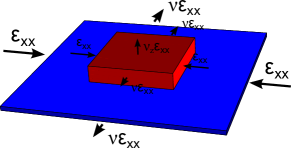
Figure 7: The first example of an experimental setup, where samples which have the same alignment of their crystalline $a-b$ axes are glued at several different angles to a piezoelectric stack.

We now consider the relation (50) for the rotated sample and in the absence of in-plane mirror symmetries. We align our coordinate system axes with the rectangular crystal edges and therefore along the $a,b$ crystal axes. In this system, the elastoresistance and elastic stiffness are given by the expressions in (51) and the strain $\boldsymbol{\epsilon}_{\text{crystal}}$ seen by the crystal is related to the strain in the coordinate system of the piezo by a rotation

$$\boldsymbol{\epsilon}_{\text{crystal}} =\hat{R}\hat{\alpha}_{\theta}\hat{R}^{-1}\,\boldsymbol{\epsilon}_{\text{piezo}}\,.$$ (53)

Here, we defined the relation between the real and the engineering strain $\hat{R}=\text{diag}(1,1,1,2,2,2)$ and the rotation matrix for the 6-component arrays similar to Ref. [Kuo1, ]:

$$\alpha_{\theta}=\left(\begin{matrix}\cos^{2}(\theta)&\sin^{2}(\theta)&0&0&0&2\cos(\theta)\sin(\theta)\\ \sin^{2}(\theta)&\cos^{2}(\theta)&0&0&0&-2\cos(\theta)\sin(\theta)\\ 0&0&1&0&0&0\\ 0&0&0&\cos(\theta)&-\sin(\theta)&0\\ 0&0&0&\sin(\theta)&\cos(\theta)&0\\ -\cos(\theta)\sin(\theta)&\cos(\theta)\sin(\theta)&0&0&0&\cos^{2}(\theta)-\sin^{2}(\theta)\end{matrix}\right),$$ (54)

The strain in the piezo system is given by $\boldsymbol{\epsilon}_{\text{piezo}}=(1,-\nu_{p},-\nu_{z}(\theta),0,0,0)\epsilon_{xx}$. Note, that due to the crystal axis rotation the Poisson ratio $\nu_{z}(\theta)$ of the crystal in $z$ direction now depends on the rotation angle $\theta$ (see Fig. 7). The angular dependence can be derived by considering the stress-strain relation $\boldsymbol{\tau}_{\text{crystal}}=\hat{C}\boldsymbol{\epsilon}_{\text{crystal}}$ and the condition $\tau_{3,\text{crystal}}=\tau_{zz,\text{crystal}}=0$ since there is no applied stress in $z$ direction of the crystal. One finds that

$$\nu_{z}(\theta)=\frac{C_{13}\left(\cos^{2}(\theta)-\nu\sin^{2}(\theta)\right)+C_{23}\left(\sin^{2}(\theta)-\nu\cos^{2}(\theta)\right)-C_{36}(\nu+1)\sin(2\theta)}{C_{33}}.$$ (55)

The resistance change $\delta\textbf{{r}}$ is therefore given by

$$\delta\textbf{{r}}=\hat{m}\boldsymbol{\epsilon}_{\text{crystal}}=\hat{m}\hat{R}\hat{\alpha}_{\theta}\hat{R}^{-1}\,\boldsymbol{\epsilon}_{\text{piezo}},$$ (56)

such that the measured $xx$-component is given by

$$\delta r_{1}(\theta)=\left(\frac{\Delta R}{R}\right)_{xx}\kern-10.00002pt(\theta) =\biggl{(}m_{11}\bigl{[}\cos^{2}(\theta)-\nu_{p}\sin^{2}(\theta)\bigr{]}+m_{12}\bigl{[}\sin^{2}(\theta)-\nu_{p}\cos^{2}(\theta)\bigr{]}$$

$$\quad-m_{16}(\nu_{p}+1)\sin(2\theta)-m_{13}\nu_{z}(\theta)\biggr{)}\cdot\epsilon_{xx}.$$ (57)

Looking at the odd contribution we finally find

$$\left(\frac{\Delta R}{R}\right)^{\text{odd}}_{xx}\kern-10.00002pt(\theta) =\frac{1}{2}\left[\left(\frac{\Delta R}{R}\right)_{xx}\kern-10.00002pt(\theta)-\left(\frac{\Delta R}{R}\right)_{xx}\kern-10.00002pt(-\theta)\right]=(\nu_{p}+1)\,\biggl{[}\frac{m_{xx,zz}C_{zz,xy}}{C_{zz,zz}}-m_{xx,xy}\biggr{]}\sin(2\theta)\cdot\epsilon_{xx}.$$

E.3 Setup 2

The second proposed setup is similar to the one described in the previous section, but here we start from a thin film crystal and use lithography to cut out the rectangular sections as shown in Fig. 8. The advantage of this method is that aligning the crystal by gluing it on the piezo element with high precision is a rather difficult task, whereas in using lithography, one can cut out the samples very precisely.

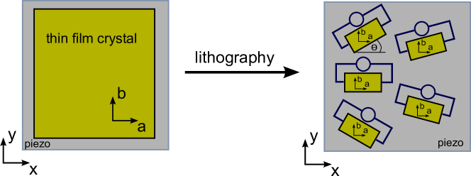
Figure 8: A second possible experimental setup, where crystals with different alignment of their crystalline axes can onto the piezoelectric stack.

In contrast to the other experiment, the crystal axes $a,b$ are aligned with the principal axes of the piezo stack. Therefore, the Poisson ratio in $z$ direction does not depend on the angle of the cut. If we consider the coordinate system to be along the $a,b$ (and thus also $x,y$) axis, what is measured is effectively the rotated resistance

$$\delta\textbf{{r}}(\theta)=\hat{\alpha}_{\theta}\delta\textbf{{r}}_{0}=\hat{\alpha}_{\theta}\hat{m}\cdot\boldsymbol{\epsilon}_{\text{piezo}}.$$ (58)

The measured longitudinal resistance is therefore given by

$$\delta r_{1}(\theta)=\ \left(\frac{\Delta R}{R}\right)_{xx}\kern-10.00002pt(\theta) =\biggl{(}\cos^{2}(\theta)\bigl{[}m_{11}-\nu m_{12}-\nu_{z}m_{13}\bigr{]}+\sin^{2}(\theta)\bigl{[}m_{21}-\nu m_{22}-\nu_{z}m_{23}\bigr{]}$$

$$\qquad-\sin(2\theta)\bigl{[}m_{61}-\nu m_{62}-\nu_{z}m_{63}\bigr{]}\biggr{)}\epsilon_{xx},$$ (59)

and the antisymmetric part

$$\left(\frac{\Delta R}{R}\right)^{\text{odd}}_{xx}\kern-10.00002pt(\theta)=-\sin(2\theta)\bigl{[}m_{61}-\nu m_{62}-\nu_{z}m_{63}\bigr{]}\epsilon_{xx},$$ (60)

is again proportional to $\sin(2\theta)$ and only present for broken mirror symmetries.

References

• (1) C. M. Varma, Phys. Rev. Lett. 83, 3538 (1999).
• (2) C. M. Varma, Phys. Rev. B 73, 155113 (2006).
• (3) S. Chakravarty, R. Laughlin, D. K. Morr, and C. Nayak, Physical Review B 63, 094503 (2001).
• (4) R. Laughlin, Physical Review Letters 112, 017004 (2014).
• (5) J. Zaanen and O. Gunnarsson, Physical Review B 40, 7391 (1989).
• (6) K. Machida, Physica C: Superconductivity 158, 192 (1989).
• (7) V. Emery and S. Kivelson, Physica C: Superconductivity 209, 597 (1993).
• (8) V. Emery, S. Kivelson, and J. Tranquada, Proceedings of the National Academy of Sciences 96, 8814 (1999).
• (9) S. R. White and D. Scalapino, Physical Review Letters 80, 1272 (1998).
• (10) S. Sachdev and R. La Placa, Physical Review Letters 111, 027202 (2013).
• (11) K. Efetov, H. Meier, and C. Pépin, Nature Physics 9, 442 (2013).
• (12) Y. Wang and A. Chubukov, Physical Review B 90, 035149 (2014).
• (13) D. Chowdhury and S. Sachdev, Phys. Rev. B 90, 245136 (2014).
• (14) A. V. Maharaj, P. Hosur, and S. Raghu, Phys. Rev. B 90, 125108 (2014).
• (15) L. Nie, G. Tarjus, and S. A. Kivelson, Proceedings of the National Academy of Sciences 111, 7980 (2014).
• (16) E. Berg, E. Fradkin, and S. A. Kivelson, Physical Review B 79, 064515 (2009).
• (17) P. A. Lee, Physical Review X 4, 031017 (2014).
• (18) D. F. Agterberg, D. S. Melchert, and M. K. Kashyap, Phys. Rev. B 91, 054502 (2015).
• (19) J.-H. Chu, H.-H. Kuo, J. G. Analytis, and I. R. Fisher, Science 337, 710 (2012), http://www.sciencemag.org/content/337/6095/710.full.pdf.
• (20) H.-H. Kuo, M. C. Shapiro, S. C. Riggs, and I. R. Fisher, Phys. Rev. B 88, 085113 (2013).
• (21) H.-H. Kuo and I. R. Fisher, Phys. Rev. Lett. 112, 227001 (2014).
• (22) S. C. Riggs et al., Nature Communications 6, 6425 (2015).
• (23) C. Lupien et al., Phys. Rev. Lett. 86, 5986 (2001).
• (24) Also the Hall conductivity can be calculated using the presented formalism. Note that in this case one has to use a different response than (3).
• (25) Since we are calculating the DC conductivity, we have to assume a finite scattering time $1/\tau_{\text{sc}}\ll\mu$, where $\mu$ is the chemical potential, so that the spectral functions are sharply peaked Lorentzians rather than delta functions.
• (26) V. M. Pereira, A. H. Castro Neto, and N. M. R. Peres, Phys. Rev. B 80, 045401 (2009).
• (27) J. Tranquada, B. Sternlieb, J. Axe, Y. Nakamura, and S. Uchida, Nature 375, 561 (1995).
• (28) J. Hoffman et al., Science 295, 466 (2002).
• (29) C. Howald, H. Eisaki, N. Kaneko, M. Greven, and A. Kapitulnik, Physical Review B 67, 014533 (2003).
• (30) G. Ghiringhelli et al., Science 337, 821 (2012).
• (31) J. Chang et al., Nature Physics 8, 871 (2012).
• (32) N. Doiron-Leyraud et al., Physical Review X 3, 021019 (2013).
• (33) A. Allais, J. Bauer, and S. Sachdev, Physical Review B 90, 155114 (2014).
• (34) A. Thomson and S. Sachdev, Phys. Rev. B 91, 115142 (2015).
• (35) T. Wu et al., Nature 477, 191 (2011).
• (36) M. Gurvitch and A. T. Fiory, Phys. Rev. Lett. 59, 1337 (1987).
• (37) H. Ding et al., NATURE 382, 51 (1996).
• (38) T. Timusk and B. Statt, Reports on Progress in Physics 62, 61 (1999).
• (39) B. Fauqué et al., Phys. Rev. Lett. 96, 197001 (2006).
• (40) Y. Li et al., Nature 455, 372 (2008).
• (41) Y. Li et al., Nature 468, 283 (2010).
• (42) S. Tewari, C. Zhang, V. M. Yakovenko, and S. Das Sarma, Phys. Rev. Lett. 100, 217004 (2008).
• (43) V. Aji, Y. He, and C. Varma, Physical Review B 87, 174518 (2013).
• (44) V. M. Yakovenko, Physica B: Condensed Matter 460, 159 (2015).
• (45) C. Varma, EPL (Europhysics Letters) 106, 27001 (2014).
• (46) J. Xia et al., Phys. Rev. Lett. 100, 127002 (2008).
• (47) Y. Lubashevsky, L. Pan, T. Kirzhner, G. Koren, and N. P. Armitage, Phys. Rev. Lett. 112, 147001 (2014).
• (48) A. Shekhter and C. Varma, Physical Review B 80, 214501 (2009).
• (49) Note that the same symmetry arguments can be applied to either the shear conductivity or shear resistivity and moreover $\Gamma_{xx,xy}\not=0\Leftrightarrow m_{xx,xy}\not=0$.
• (50) G. D. Mahan, Many-particle physics (Springer Science & Business Media, 2000).
• (51) The elastoresistance $m_{\alpha\beta,\gamma\delta}=\partial R_{\alpha\beta}/\partial\epsilon_{\gamma\delta}$ is symmetric in the first two indices due to Onsager’s relation $R_{\alpha\beta}(\textbf{{H}})=R_{\beta\alpha}(\textbf{{H}})$ (in the absence of a magnetic field H) and in the last two indices due to the symmetric definition of the strain tensor $\epsilon_{\gamma\delta}=\epsilon_{\delta\gamma}$.
• (52) Note that the elastic stiffness has the more general symmetry $C_{\alpha\beta,\gamma\delta}=C_{\beta\alpha,\gamma\delta}=C_{\alpha\beta,\delta\gamma}=C_{\gamma\delta,\alpha\beta}$ since it can be written as the second derivative of the free energy with respect to strain: $C_{\alpha\beta,\gamma\delta}=\frac{\partial^{2}F}{\partial\epsilon_{\alpha\beta}\partial\epsilon_{\gamma\delta}}$.