Optical Signatures of Non-Markovian Behaviour in Open Quantum Systems

Abstract

We derive an extension to the quantum regression theorem which facilitates the calculation of two-time correlation functions and emission spectra for systems undergoing non-Markovian evolution. The derivation exploits projection operator techniques, with which we obtain explicit equations of motion for the correlation functions, making only a second order expansion in the system–environment coupling strength, and invoking the Born approximation at a fixed initial time. The results are used to investigate a driven semiconductor quantum dot coupled to an acoustic phonon bath, where we find the non-Markovian nature of the dynamics has observable signatures in the form of phonon sidebands in the resonance fluorescence emission spectrum. Furthermore, we use recently developed non-Markovianity measures to demonstrate an associated flow of information from the phonon bath back into the quantum dot exciton system.

I Introduction

Two-time correlation functions are quantities of frequent interest in many areas of physics. This is particularly true in quantum optics, where correlation functions of the form $\langle A(t_{1})B(t_{2})\rangle$ give the field correlation properties of an emitting system such as a driven atom, and whose Fourier transform gives the measured spectrum Mollow (1969). If the governing Hamiltonian can be diagonalised exactly, calculation of the two-time correlation function is no more challenging than calculating a one-time expectation value of the form $\langle A(t_{1})\rangle$. However, it is more often the case that the emitting system is an open system, whose dynamics can only be approximated. In this case, since the system operators $A$ and $B$ are evaluated at two distinct times, calculation of the correlation function given knowledge of system dynamics alone is not at first sight straightforward. The quantum regression theorem, however, gives a prescription of how such correlation functions can be related to more readily obtainable system expectation values Carmichael (1998). A subtle caveat of the quantum regression theorem, however, is that it applies only to systems undergoing strictly Markovian evolution. It requires that the complete density operator of the system and environment factorises at all times, and that the reduced system density operator obeys a time-independent master equation Swain (1999); Alonso and de Vega (2005); de Vega and Alonso (2008); Flindt et al. (2008); Budini (2008); Goan et al. (2010, 2011); Guarnieri et al. (2014).

The requirement of Markovian evolution is typically fulfilled in the traditional case of atomic quantum optics due to the extremely short correlation time of the electromagnetic environment Mandel and Wolf (1995); Koshino and Shimizu (2004). However, more recent technological advances in the fabrication of artificial emitters and the engineering of structured environments have given rise to systems whose evolution is not purely Markovian, yet whose properties are typically probed optically. These systems include semiconductor quantum dots (QDs), for which Rabi oscillations Flagg et al. (2009); Ramsay et al. (2010); Monniello et al. (2013), resonance fluorescence Ates et al. (2009); Ulrich et al. (2011); Wei et al. (2014); Matthiesen et al. (2012, 2013), and single photon emission Michler et al. (2000); Santori et al. (2002); Flagg et al. (2010) have all been demonstrated. QDs, however, exist in a solid-state substrate, and interactions with phonons and nuclear spins can modify their emission properties McCutcheon and Nazir (2013); Monniello et al. (2013); Roy and Hughes (2011); Roy-choudhury and Hughes (2015) and also give rise to non-Markovian behaviour McCutcheon and Nazir (2010); Kaer and Mørk (2014); Cywiński et al. (2009); Barnes et al. (2012); Ubbelohde et al. (2012). Additionally, for technological applications, such as indistinguishable and entangled photon sources Lindner and Rudolph (2009); Gazzano et al. (2013); Müller et al. (2014); McCutcheon et al. (2014), it is often desirable to place artificial emitters in structured photonic environments such as in photonic crystals or micro-pillar cavities, which also have the potential to lead to non-Markovian behaviour.

Thus, in order to model the optical properties of these ever more exotic systems, it is important to establish how two-time correlation functions can be calculated for open systems undergoing non-Markovian evolution. We note that efforts in this direction have been made Swain (1999); Alonso and de Vega (2005); de Vega and Alonso (2008); Flindt et al. (2008); Budini (2008); Goan et al. (2010, 2011); Guarnieri et al. (2014), and the conditions under which the regression theorem holds have been scrutinised Budini (2008). Many of these, however, rely on a number of uncontrolled approximations, such as artificially enforcing time-locality Goan et al. (2010, 2011), or assuming a restrictive (rotating wave-like) form of the system–environment coupling Alonso and de Vega (2005); de Vega and Alonso (2008). Additionally, it is not clear to what extent non-Markovian behaviour has any measurable optical consequences in physically relevant systems.

In this work we use projection operator techniques to derive a non-Markovian extension to the quantum regression theorem, valid to second order in the system–environment coupling strength, and invoking the Born approximation only at a single fixed initial time. The second order expansion restricts the theory to weak–system environment coupling regimes for which non-Markovian behaviour is typically only present for short times, and which is usually very challenging to observe. The key advantage of the present work, however, is that this short-time behaviour is of a two-time correlation function, whose spectral counterpart corresponds to a concrete readily measurable quantity. Specifically, we apply our formalism to the relevant case of a driven QD Ates et al. (2009); Ulrich et al. (2011); Wei et al. (2014); Matthiesen et al. (2012, 2013), and find that the experimentally observed phonon sidebands in the emission spectra are a direct consequence of non-Markovian behaviour, which the standard Markovian treatment fails to capture. Moreover, we confirm true non-Markovianity and indivisibility of the underlying dynamical map by demonstrating that the phonon sidebands are associated with a flow of information from the phonon environment back into the QD system Breuer et al. (2009).

II Two-time correlation functions and the Regression Theorem

We begin by introducing two-time correlation functions and the standard (Markovian) regression theorem. We consider a system $S$ interacting with an environment $E$, and wish to calculate two-time correlation functions of the form $G(t,\tau)=\langle A(t+\tau)B(t)\rangle=\mathrm{Tr}_{S+E}\big{[}A(t+\tau)B(t)\chi(0)\big{]}$, where $A$ and $B$ are system operators, $\chi(0)$ is the total system-plus-environment state at $t=0$, and $\mathrm{Tr}_{S+E}$ denotes a trace over both $S$ and $E$. For a time independent Hamiltonian $H$ we have $A(t)=U^{\dagger}(t)AU(t)$ with $U(t)=\exp[-iHt]$ (we set $\hbar=1$), and using the cyclic property of the trace we find

$$G(t,\tau) =\mathrm{Tr}_{S}\big{[}A\,\Lambda(t,\tau)\big{]},$$ (1)

where the system operator $$\Lambda(t,\tau)$$ is given by

$$\Lambda(t,\tau) =\mathrm{Tr}_{E}\big{[}U(\tau)B\chi(t)U^{\dagger}(\tau)\big{]},$$ (2)

with $\chi(t)=U(t)\chi(0)U^{\dagger}(t)$. From Eq. (1) we see that calculation of $G(t,\tau)$ amounts to calculating something analogous to the expectation value of $A$, but with respect to the operator $\Lambda(t,\tau)$ rather than the reduced system density operator $\rho(t)=\mathrm{Tr}_{E}[U(t)\chi(0)U^{\dagger}(t)]$. For this reason we refer to $\Lambda(t,\tau)$ as the reduced effective density operator, and $\rho(t)$ the reduced physical density operator.

The standard regression theorem proceeds by observing that the definition of the effective density operator $\Lambda(t,\tau)$ in Eq. (2) bares a strong resemblance to that of the reduced physical density operator, $\rho(t)=\mathrm{Tr}_{E}[U(t)\chi(0)U^{\dagger}(t)]$. As such, if we know the equation of motion for the physical density operator with respect to $t$, say $\partial_{t}\rho(t)=\Phi\rho(t)$, then the reduced effective density operator will obey the same equation of motion but with respect to $\tau$, and with a modified initial condition, namely $\partial_{\tau}\Lambda(t,\tau)=\Phi\Lambda(t,\tau)$ and $\Lambda(t,0)=B\rho(t)$. We will see, however, that this procedure contains a hidden assumption that the total physical density operator $\chi(t)$ factorises for all times Swain (1999); Alonso and de Vega (2005); de Vega and Alonso (2008); Goan et al. (2010).

II.1 Effective Density Operator Master Equation Using Projection Operators

To see how this assumption arises, and how it can be removed, we now derive the quantum regression theorem using the projection operator formalism Breuer and Petruccione (2002); Nakajima (1958); Zwanzig (1960); Shibata et al. (1977). This well-established formalism was originally developed to calculate physical density operator master equations, and our purpose here is to do the same for the effective density operator, taking particular care to identify places where any approximations have different physical significance. To begin we must establish an interaction picture for the total effective density operator, which we define as $\Upsilon(t,\tau)=U(\tau)B\chi(t)U^{\dagger}(\tau)$, such that $\smash{\Lambda(t,\tau)=\mathrm{Tr}_{E}[\Upsilon(t,\tau)]}$. We write the total Hamiltonian $H=H_{0}+\alpha H_{I}$, where $H_{0}=H_{S}+H_{E}$ with $H_{S}$ and $H_{E}$ acting exclusively on $S$ and $E$ respectively. We recall that the unitary operators $U(\tau)$ and $U_{0}(\tau)$ are defined as the solutions to the differential equations $i\partial_{\tau}U(\tau)=HU(\tau)$ and $i\partial_{\tau}U_{0}(\tau)=H_{0}U_{0}(\tau)$, and the interaction picture effective density operator as $\tilde{\Upsilon}(t,\tau)=U_{I}(\tau)B\chi(t)U_{I}^{\dagger}(\tau)$ with $U_{I}(\tau)=U_{0}^{\dagger}(\tau)U(\tau)$. From these definitions we find

$$\partial_{\tau}\tilde{\Upsilon}(t,\tau)=-i\alpha[\tilde{H}_{I}(\tau),\tilde{\Upsilon}(t,\tau)]=\alpha\mathcal{L}(\tau)\tilde{\Upsilon}(t,\tau),$$ (3)

where $\tilde{H}_{I}(\tau)=U_{0}^{\dagger}(\tau)H_{I}U_{0}(\tau)$ and the Liouvillian $\mathcal{L}(\tau)$ is defined to satisfy the second equality. We naturally define $\tilde{\Lambda}(t,\tau)=\mathrm{Tr}_{E}[\tilde{\Upsilon}(t,\tau)]$, and note that since we can write $U_{0}(\tau)=U_{S}(\tau)U_{E}(\tau)$ with the subscripts indicating whether the operators act on $S$ or $E$ we find $\Lambda(t,\tau)=U_{S}(\tau)\tilde{\Lambda}(t,\tau)U_{S}^{\dagger}(\tau)$. The Schrödinger and interaction picture equations of motion are then related through

$$\partial_{\tau}\Lambda(t,\tau)=i[\Lambda(t,\tau),H_{S}]+U_{S}(\tau)\big{(}\partial_{\tau}\tilde{\Lambda}(t,\tau)\big{)}U_{S}^{\dagger}(\tau).$$ (4)

These results demonstrate that the effective density operator has a well-defined interaction picture which facilitates the use of the master equation techniques below.

We now introduce the projection operators $\mathcal{P}$ and $\mathcal{Q}=(\openone-\mathcal{P})$, which are defined through Nakajima (1958); Zwanzig (1960); Shibata et al. (1977)

$$\mathcal{P}\tilde{\Upsilon}(t,\tau)=\mathrm{Tr}_{E}[\tilde{\Upsilon}(t,\tau)]\otimes\rho_{R}=\tilde{\Lambda}(t,\tau)\otimes\rho_{R},$$ (5)

where $\rho_{R}$ is a reference state of the environment. The projection operators project the effective density operator into factorising and non-factorising components, i.e. we can write $\tilde{\Upsilon}(t,\tau)=(\mathcal{P}+\mathcal{Q})\tilde{\Upsilon}(t,\tau)$, where the first term factorises by definition, while the second captures those components which do not. From these basic definitions one can show that $\mathcal{P}^{2}=\mathcal{P}$ and $\mathcal{Q}^{2}=\mathcal{Q}$, while $\mathcal{Q}\mathcal{P}=\mathcal{P}\mathcal{Q}=0$. In what follows we assume $\mathrm{Tr}_{E}[H_{I}\rho_{R}]=0$. This is not an approximation, since if $\mathrm{Tr}_{E}[H_{I}\rho_{R}]=\langle H_{I}\rangle\neq 0$ we can redefine $H_{S}^{\prime}=H_{S}+\langle H_{I}\rangle$ and $H_{I}^{\prime}=H_{I}-\langle H_{I}\rangle$ leaving the total Hamiltonian unchanged, and we then have $\mathrm{Tr}_{E}[H_{I}^{\prime}\rho_{E}]=0$ by definition McCutcheon et al. (2011); Jang (2009). Provided our reference state is chosen such that $[H_{E},\rho_{E}]=0$, valid for e.g. thermal states, we find $\mathrm{Tr}_{E}[\tilde{H}_{I}^{\prime}(\tau)\rho_{R}]=0$ which implies $\mathcal{P}\mathcal{L}(\tau)\mathcal{P}=0$.

Now, our aim is to derive an equation of motion for the factorising part of the effective density operator $\mathcal{P}\tilde{\Upsilon}(t,\tau)$, from which we can readily obtain $\Lambda(t,\tau)=\mathrm{Tr}_{E}[\mathcal{P}\tilde{\Upsilon}(t,\tau)]$, and using Eq. (1) calculate the two-time correlation function. Following Ref. Breuer and Petruccione (2002) we act with both $\mathcal{P}$ and $\mathcal{Q}$ on Eq. (3) yielding two differential equations which we must solve simultaneously. Inserting $\openone=\mathcal{P}+\mathcal{Q}$ on the right hand side and using $\mathcal{P}\mathcal{L}(\tau)\mathcal{P}=0$ the first of these becomes

$$\partial_{\tau}\mathcal{P}\tilde{\Upsilon}(t,\tau)=\alpha\mathcal{P}\mathcal{L}(\tau)\mathcal{Q}\tilde{\Upsilon}(t,\tau),$$ (6)

while the second involving $\partial_{\tau}\mathcal{Q}\tilde{\Upsilon}(t,\tau)$ can be formally integrated to give

$$\mathcal{Q}\tilde{\Upsilon}(t,\tau)= \,\,G_{F}(\tau,0)\mathcal{Q}\tilde{\Upsilon}(t,0)$$

$$+ \,\,\alpha\int_{0}^{\tau}\mathrm{d}sG_{F}(\tau,s)\mathcal{Q}\mathcal{L}(s)\mathcal{P}\tilde{\Upsilon}(t,s),$$ (7)

where $G_{F}(\tau,s)=\mathrm{T}_{\leftarrow}\exp\left[\alpha\int_{s}^{\tau}\mathrm{d}s^{\prime}\mathcal{Q}\mathcal{L}(s^{\prime})\right]$ with $\mathrm{T}_{\leftarrow}$ the chronological time ordering operator Breuer and Petruccione (2002). To obtain a time-local form, from Eq. (3) we see that we can write $\tilde{\Upsilon}(t,s)=G_{B}(\tau,s)\tilde{\Upsilon}(t,\tau)$, where $G_{B}(\tau,s)=\mathrm{T}_{\rightarrow}\exp\left[-\alpha\int_{s}^{\tau}\mathrm{d}s^{\prime}\mathcal{L}(s^{\prime})\right]$ with $\mathrm{T}_{\rightarrow}$ the anti-chronological time ordering operator. From Eq. (7) we then find

$$(\openone-\Sigma(\tau))\mathcal{Q}\tilde{\Upsilon}(t,\tau)=G_{F}(\tau,0)\mathcal{Q}\tilde{\Upsilon}(t,0)+\Sigma(\tau)\mathcal{P}\tilde{\Upsilon}(t,\tau),$$ (8)

where $\Sigma(\tau)=\alpha\int_{0}^{\tau}\mathrm{d}sG_{F}(\tau,s)\mathcal{Q}\mathcal{L}(s)\mathcal{P}G_{B}(\tau,s)$. Provided the inverse of the operator $(\openone-\Sigma(\tau))$ exists, Eq. (8) can be solved for $\mathcal{Q}\tilde{\Upsilon}(t,\tau)$. Since we are ultimately interested in the weak-coupling limit of the system–environment interaction $\alpha$, and since $\Sigma(\tau)$ contains no zeroth order term in $\alpha$, we assume the existence of such an operator, and in solving for $\mathcal{Q}\tilde{\Upsilon}(t,\tau)$ we obtain

$$\mathcal{Q}\tilde{\Upsilon}(t,\tau)= \,(\openone-\Sigma(\tau))^{-1}\Sigma(\tau)\mathcal{P}\tilde{\Upsilon}(t,\tau)$$

$$+ \,(\openone-\Sigma(\tau))^{-1}G_{F}(\tau,0)\mathcal{Q}\tilde{\Upsilon}(t,0).$$ (9)

Inserting this formal solution for the non-factorising component of the effective density operator into Eq. (6) for the factorising component we find

$$\partial_{\tau}\mathcal{P}\tilde{\Upsilon}(t,\tau)=\mathcal{I}(\tau)\mathcal{Q}\tilde{\Upsilon}(t,0)+\mathcal{K}(\tau)\mathcal{P}\tilde{\Upsilon}(t,\tau),$$ (10)

where we have defined the kernels

$$\mathcal{I}(\tau) =\alpha\mathcal{P}\mathcal{L}(\tau)(\openone-\Sigma(\tau))^{-1}G_{F}(\tau,0)\mathcal{Q},$$ (11)

$$\mathcal{K}(\tau) =\alpha\mathcal{P}\mathcal{L}(\tau)(\openone-\Sigma(\tau))^{-1}\Sigma(\tau)\mathcal{P}.$$ (12)

These expressions constitute an exact equation of motion for the reduced effective density operator, with an inhomogeneous term which depends on the physical density operator through $\mathcal{Q}\tilde{\Upsilon}(t,0)=\mathcal{Q}B\chi(t)$.

For these reasons, it what follows it will be useful to also consider the evolution for the factorising and non-factorising parts of the physical density operator $\chi(t)$. For this purpose we use the projection operator methods outlined above, and we find that the derivation proceeds in precisely the same manner, the only difference being that the time argument $\tau$ is replaced with $t$ and the initial condition is $(\mathcal{P}+\mathcal{Q})\chi(0)$. In exact analogy with Eq. (9), we find that the non-factorising part has solution

$$\mathcal{Q}\tilde{\chi}(t)= \,(\openone-\Sigma(t))^{-1}\Sigma(t)\mathcal{P}\tilde{\chi}(t)$$

$$+ \,(\openone-\Sigma(t))^{-1}G_{F}(t,0)\mathcal{Q}\tilde{\chi}(0),$$ (13)

leading to the equation of motion

$$\partial_{t}\mathcal{P}\tilde{\chi}(t)=\mathcal{I}(t)\mathcal{Q}\tilde{\chi}(0)+\mathcal{K}(t)\mathcal{P}\tilde{\chi}(t),$$ (14)

with the kernels again given by Eqs. (11) and (12).

II.2 Removal of the Born Approximation and the Non-Markovian Regression Theorem

Returning to Eq. (10) for the effective density operator, we now consider the inhomogeneous term $\mathcal{I}(\tau)\mathcal{Q}\tilde{\Upsilon}(t,0)$. If we were to make the Born approximation, and assume that the physical density operator factorises at all times, $\chi(t)\approx\rho(t)\otimes\rho_{R}$, then $\mathcal{Q}\tilde{\Upsilon}(t,0)=0$ and the inhomogeneous term vanishes. Analogously, in Eq. (14) we see that in assuming factorising initial conditions, $\chi(0)\approx\rho(0)\otimes\rho_{R}$, the inhomogeneous term for the physical density operator vanishes. In these cases the equations of motion for the effective and the physical density operator become identical, i.e. we have $\partial_{t}\mathcal{P}\tilde{\chi}(t)=\mathcal{K}(t)\mathcal{P}\tilde{\chi}(t)$ and $\partial_{\tau}\mathcal{P}\tilde{\Upsilon}(t,\tau)=\mathcal{K}(\tau)\mathcal{P}\tilde{\Upsilon}(t,\tau)$. We conclude that we must make the Born approximation at all times for the standard regression theorem to apply.

We now turn to the key insight of this work which allows us to remove the Born approximation. Since $B$ is a system operator, and assuming $[H_{E},\rho_{R}]=0$, it can be shown that $\mathcal{Q}\tilde{\Upsilon}(t,0)=B\mathcal{U}(t)\mathcal{Q}\tilde{\chi}(t)$, where $\mathcal{U}_{0}(t)\tilde{\chi}(t)=\smash{U_{0}(t)\tilde{\chi}(t)U_{0}^{\dagger}(t)}$. The object $\mathcal{Q}\tilde{\chi}(t)$ represents deviations from factorability of the physical density operator. However, we already have an exact form for this, namely Eq. (13). Assuming factorising initial conditions only, the second term in Eq. (13) is zero, and using what remains in Eq. (10) gives

$$\partial_{\tau}\mathcal{P}\tilde{\Upsilon}(t,\tau)=\mathcal{I}^{\prime}(t,\tau)\mathcal{P}\tilde{\chi}(t)+\mathcal{K}(\tau)\mathcal{P}\tilde{\Upsilon}(t,\tau),$$ (15)

where the new inhomogeneous term is given by $\mathcal{I}^{\prime}(t,\tau)=\mathcal{I}(\tau)\mathcal{Q}B\mathcal{U}_{0}(t)(\openone-\Sigma(t))^{-1}\Sigma(t)\mathcal{P}$. Eq. (15) is an exact equation of motion for the reduced effective density operator, in which the inhomogeneous term depends on the reduced physical density operator, which obeys the exact equation of motion Eq. (14) with $\mathcal{Q}\tilde{\chi}(0)=0$.

Though Eqs. (15) and (14) are exact, calculating explicit forms for the kernels is difficult. The utility of the projection operator approach used here is that it allows for a systematic expansion in the system–environment coupling strength $\alpha$. Expanding the kernels appearing in Eq. (15) to second order in $\alpha$ and moving back into the Schrödinger picture we find

$$\!\!\!\partial_{\tau}\Lambda(t,\tau)\!=i[\Lambda(t,\tau),H_{S}]+\mathcal{D}(\Lambda(t,\tau))+\mathcal{C}(\varrho(t,\tau)),$$ (16)

where the effective density operator enters through

$$\!\!\!\mathcal{D}(\Lambda(t,\tau))=-\int_{0}^{\tau}\!\!\mathrm{d}s\mathrm{Tr}_{E}\big{[}H_{I},\big{[}\tilde{H}_{I}(-s),\Lambda(t,\tau)\rho_{R}\big{]}\big{]},$$ (17)

and the physical density operator enters through

$$\mathcal{C}(\varrho(t, \tau))=$$

$$- \int_{\tau}^{\tau+t}\!\!\!\!\mathrm{d}s\mathrm{Tr}_{E}\big{[}H_{I},\tilde{B}(-\tau)\big{[}\tilde{H}_{I}(-s),\varrho(t,\tau)\rho_{R}\big{]}\big{]},$$ (18)

with $\varrho(t,\tau)=U_{S}(\tau)\rho(t)U_{S}^{\dagger}(\tau)$, $\tilde{B}(-\tau)=U_{S}(\tau)BU_{S}^{\dagger}(\tau)$, and we have absorbed factors of $\alpha$ into the interaction Hamiltonians, i.e. $\alpha H_{I}\to H_{I}$. Let us review what approximations have been made. We assumed factorising initial conditions, $\chi(0)=\rho(0)\otimes\rho_{R}$, and expanded the kernels to second order in the system-environment coupling strength. From this point onwards no further approximations are necessary. Finally, we note that $\rho(t)$ entering Eq. (18) can be found at no additional cost since to the same level of approximation we have $\partial_{t}\rho(t)=-i[H_{S},\rho(t)]+\mathcal{D}(\rho(t))$.

Before proceeding, we note that we can obtain a time-independent equation of motion for $\Lambda(t,\tau)$ by making a Markovian approximation and let $\tau\to\infty$ in Eq. (16). We then find $\mathcal{C}(\varrho(t,\tau))=0$ and the inhomogeneous term disappears. In this case the regression theorem is recovered since $\rho(t)$ and $\Lambda(t,\tau)$ obey the same equation of motion. Recalling that we also find $\mathcal{C}(\varrho(t,\tau))=0$ when making the Born approximation, $\chi(t)\approx\rho(t)\otimes\rho_{R}$, we conclude that in the present context the Markovian approximation cannot be made without also implicitly making the Born approximation. Is the converse also true? Is it possible to not make the Markovian approximation by leaving the integration limit in Eq. (16) at $\tau$, yet at the same time make the Born approximation and neglect the inhomogeneous term $\mathcal{C}(\varrho(t,\tau))$? This is what one would obtain naively applying the regression theorem to a non-Markovian master equation for the physical density operator. In the following we will see that this approach is ill-advised and can give rise to unphysical results.

III Application to a Driven Semiconductor Quantum Dot Coupled to Acoustic Phonons

We now use our results and consider a driven semiconductor QD in a non-Markovian acoustic phonon environment Ramsay et al. (2010); McCutcheon and Nazir (2010, 2013). The QD is described by ground and single exciton states $\left|g\right\rangle$ and $\left|e\right\rangle$, and the laser by a constant Rabi frequency $\Omega$ and detuning $\delta$. In a rotating frame, and within the dipole and rotating wave approximations the Hamiltonian is given by $H=H_{S}+H_{I}+H_{E}$, with $H_{S}=\delta\sigma^{\dagger}\sigma+(\Omega/2)(\sigma^{\dagger}+\sigma)$, $H_{I}=\sigma^{\dagger}\sigma\sum_{k}g_{k}(b_{k}^{\dagger}+b_{k})$ and $\smash{H_{E}=\sum_{k}\omega_{k}b_{k}^{\dagger}b_{k}}$, where $\sigma=\left|g\right\rangle\hskip-2.84526pt\left\langle e\right|$, a phonon with wave vector $k$ and frequency $\omega_{k}$ is described by creation and annihilation operators $b_{k}^{\dagger}$ and $b_{k}$, and we take a thermal state for the phonon environment $\rho_{R}=\exp[-H_{E}/k_{B}T]/\mathrm{Tr}[\exp[-H_{E}/k_{B}T]]$, with $T$ the sample temperature. The exciton–phonon interaction is characterised by coupling constants $g_{k}$, which ultimately enter only through the spectral density $J(\omega)=\sum_{k}g_{k}^{2}\delta(\omega-\omega_{k})$. For coupling to longitudinal acoustic phonons we can take the form $J(\omega)=\eta\,\omega^{3}\exp[-(\omega/\omega_{c})^{2}]$, with $\eta$ the QD–phonon coupling strength, and $\omega_{c}$ the cut-off frequency, whose inverse gives the memory time of the environment McCutcheon and Nazir (2010). We tune the laser to the phonon-shifted QD transition frequency, $\delta=\int_{0}^{\infty}\mathrm{d}\omega J(\omega)/\omega$, set $\Omega=0.12~{}\mathrm{ps}^{-1}$, and use the realistic parameters $\eta=0.03~{}\mathrm{ps}^{2}$ and $\omega_{c}=2.2~{}\mathrm{ps}^{-1}$, with $T=4~{}\mathrm{K}$. The steady state first order correlation function of the QD emission is $g^{(1)}(\tau)=\lim_{t\to\infty}\langle\sigma^{\dagger}(t+\tau)\sigma(t)\rangle$, which we calculate with Eq. (16), adding a term $\Gamma(\sigma\Lambda(t,\tau)\sigma^{\dagger}-\frac{1}{2}\{\sigma^{\dagger}\sigma,\Lambda(t,\tau)\})$ with $1/\Gamma=100~{}\mathrm{ps}$ to capture spontaneous emission. Including spontaneous emission in this way assumes that the photonic environment is strictly Markovian, and is justified fully in the Appendix. Having obtained the first order correlation function the incoherent emission spectrum is defined as $S(\Delta\omega)=\mathrm{Re}[\int_{0}^{\infty}\mathrm{d}\tau(g^{(1)}(\tau)-g^{(1)}(\infty))\mathrm{e}^{-i\Delta\omega\tau}]$.

Figure 1: Real (a) and imaginary (b) parts of the first order correlation function, calculated using a Markovian approximation (solid blue), the full non-Markovian theory (dashed orange), and the non-Markovian theory but neglecting the inhomogeneous term in Eq. (18) (green dotted). Plot (c) shows the corresponding emission spectrum with the inset showing a different scale on which the Mollow triplet can be seen. From the main part of (c) it is seen that only the full non-Markovian theory correctly captures the phonon sideband at lower energies. Plot (d) shows the derivative of the trace distance between two states evolved from different initial conditions, whose positive values for times $\sim 1~{}\mathrm{ps}$ demonstrates backflow of information and true non-Markovianity.

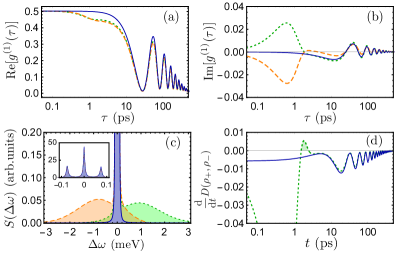
Fig. 1 shows the real (a) and imaginary part (b) of $g^{(1)}(\tau)$ calculated using the Markovian approximation (taking $\tau\to\infty$ in Eqs. (17) and (18), solid blue), the full non-Markovian theory (dashed orange), and using the naive non-Markovian theory (neglecting the inhomogeneous term in Eq. (18), dotted green). We see that for times less than the environment correlation time of $\sim 1~{}\mathrm{ps}$, all three theories predict quite distinct behaviour, reflecting the fact that non-Markovian effects are most important and these timescales. Plot (c) shows the corresponding incoherent emission spectrum, which on the inset scale displays the well-known Mollow triplet. From the main part of (c), we see that the Markovian theory, which predicts no short time oscillations, correspondingly predicts no spectral features at large frequencies. The full non-Markovian theory, however, predicts a broad sideband at lower emission frequencies. This sideband is well-known experimentally Matthiesen et al. (2013); Besombes et al. (2001); Favero et al. (2003); Ahn et al. (2005), and is attributed to phonon emission, which our theory supports. Thus, the phonon sideband in the emission spectrum is a signature of non-Markovian behaviour. This is a key feature of this work; observation of non-Markovian behaviour of one-time expectation values typically necessitates initialising a system in a well-defined state and tracking dynamics on very short timescales ($\mathrm{ps}$ in this example). Steady-state two-time correlation functions, on the other hand, capture fluctuations of a system from equilibrium. Non-Markovian behaviour of these fluctuations can be much more readily observed since their Fourier transform corresponds to an emission spectrum .

We note that while the phonon sideband has been calculated previously, it has so only in the zero driving limit $\Omega\to 0$ where the model becomes exactly solvable and the Mollow triplet is not present Besombes et al. (2001); Favero et al. (2003); Ahn et al. (2005); Roy-Choudhury and Hughes (2015). The theory presented here works for non-zero $\Omega$, allowing us to calculate the fraction of power emitted into the phonon sideband, which for the realistic parameters used here gives $\sim 10\%$, in good agreement with recent experiments Matthiesen et al. (2013).

Interestingly, it can be seen that the naive non-Markovian theory predicts a sideband at higher energies, in contrast to both intuition and experimental evidence. The inhomogeneous term in Eq. (18) which the naive approach ignores captures deviations of the true state of the environment from the reference state $\rho_{R}$ used in the master equation. For the emission spectrum, these deviations are important, since we assumed $\rho_{R}$ to be a thermal state with respect to the QD ground state, which is not the correct initial condition for an emission process. This reveals why in neglecting the inhomogeneous term the sideband incorrectly appears at higher energies; since it assumes the environment to be in equilibrium with respect to the QD ground state, it inadvertently gives dynamics which correspond more to an absorption spectrum. We note that this correspondence is only approximate, and is not expected to be a general feature.

The steady-state correlation function we have calculated captures fluctuations of the QD about its steady state, and our results suggest these fluctuations are non-Markovian in nature. In order for this is be confirmed, we calculate a non-Markovianity witness in the form of the derivative of the trace distance $D(\rho_{+},\rho_{-})=\frac{1}{2}|\rho_{+}(t)-\rho_{-}(t)|$, where $\rho_{+}(t)$ and $\rho_{-}(t)$ are physical density operator states evolved from two different initial states $\rho_{\pm}(0)=\frac{1}{2}(\openone\pm\sigma_{y})$ with $\sigma_{y}=-i\left|e\right\rangle\hskip-2.84526pt\left\langle g\right|+i\left|g\right\rangle\hskip-2.84526pt\left\langle e\right|$ Breuer et al. (2009). We are interested here in the evolution of reduced physical density operators since these characterise the behaviour of physical QD exciton, and as such use the equation of motion $\partial_{t}\rho(t)=-i[H_{S},\rho(t)]+\mathcal{D}(\rho(t))$ (i.e. without inhomogeneous term). A positive derivative of the trace distance is interpreted as a flow of information from the environment into the system, and is a sufficient condition to prove indivisibility of the underlying dynamical map, both of which can be considered definitions of non-Markovianity Breuer et al. (2009); Rivas et al. (2010); Guarnieri et al. (2014). In Fig. 1(d) we show $\frac{\mathrm{d}}{\mathrm{d}t}D(\rho_{+},\rho_{-})$ calculated using the non-Markovian theory (dotted, green), and within the Markovian approximation (solid, blue). We see that our non-Markovian theory gives rise to a time interval during which the derivative is positive, confirming true non-Markovian behaviour.

IV Summary

We have developed an extension to the quantum regression theorem, valid to second order in the system-environment coupling strength, and invoking the Born approximation at a single fixed initial time. These results have been used to demonstrate that phonon sidebands in the resonance fluorescence emission spectra of a QD are a signature of non-Markovian behaviour. In this context, it was shown that this non-Markovian behaviour is associated with a flow of information from the phonon environment back into the QD exictonic system, which is a sufficient condition to prove indivisibility of the underlying dynamical map. The projection operator method used here is an ideal starting point to include higher order system–environment coupling terms, which can in some cases lead to an exact resummation Barnes et al. (2012). Finally, it will be interesting to investigate how the results obtained here can be used to optically quantity non-Markovian behaviour Wolf et al. (2008); Breuer et al. (2009); Rivas et al. (2010); Guarnieri et al. (2014); Luoma et al. (2014).

Appendix A Effective density operator master equation for time-dependent interaction Hamiltonians

Here we give an extension to the results provided in the main text which facilitates the inclusion of time-dependent interaction Hamiltonians. For a time-dependent interaction Hamiltonian we can write the complete Schrödiner picture Hamiltonian in the form $H(t)=H_{S}+\alpha H_{I}(t)+H_{E}$. In this case defining an interaction picture proceeds analogously as in the main text, and the interaction picture equation of motion for the effective density operator again takes the form of Eq. (3), though now we have

$$\tilde{H}_{I}(\tau)=U_{0}^{\dagger}(\tau)H_{I}(\tau)U_{0}(\tau),$$ (19)

with $H_{I}(\tau)$ the Schrödinger picture interaction Hamiltonian at time $\tau$, and $\tilde{\Upsilon}(t,\tau)=U_{0}^{\dagger}(\tau)U(t+\tau,t)[B\chi(t)]U^{\dagger}(t+\tau,t)U_{0}(\tau)$ where the time evolution operator satisfies $i\partial_{t}U(t,t_{0})=H(t)U(t,t_{0})$ with $U(t_{0},t_{0})=\openone$. For this time-dependent interaction Hamiltonian the derivation of the effective density operator master equation proceeds precisely as in the main text, and we again arrive at the general expression in Eq. (15), the only difference being that the implicit occurrences of the interaction Hamiltonians are defined through Eq. (19). Expanding to second order in the system-environment coupling strength proceeds analogously, though some care must be taken when moving back into the Schrödinger picture. For a time-dependent Hamiltonian the Schrödinger picture equation of motion for the effective density again has the form $\partial_{\tau}\Lambda(t,\tau)=-i[H_{S},\Lambda(t,\tau)]+\mathcal{D}(\Lambda(t,\tau))+\mathcal{C}(\varrho(t,\tau))$, though now

$$\mathcal{D}(\Lambda(t,\tau))=$$

$$- \int_{0}^{\tau}\!\!\mathrm{d}s\mathrm{Tr}_{E}\big{[}\tilde{H}_{I}(\tau,0),\big{[}\tilde{H}_{I}(\tau-s,-s),\Lambda(t,\tau)\rho_{R}\big{]}\big{]},$$ (20)

and the inhomogeneous term is given by

$$\!\!\mathcal{C}(\rho(t))=-\!\int_{\tau}^{\tau+t}\!\!\!\!\mathrm{d}s \mathrm{Tr}_{E}\Big{[}\tilde{H}_{I}(\tau,0),\tilde{B}(-\tau)$$

$$\big{[}\tilde{H}_{I}(t+\tau-s,-s),\varrho(t,\tau)\rho_{R}\big{]}\Big{]},$$ (21)

and we have defined $\tilde{H}_{I}(t_{1},t_{2})=U_{0}^{\dagger}(t_{2})H_{I}(t_{1})U_{0}(t_{2})$. Note that in order to recover the case for a time-independent interaction Hamiltonian we simply set the first time argument in $\tilde{H}_{I}(t_{1},t_{2})$ to zero.

Appendix B Inclusion of Spontaneous Emission within the Markovian Approximation

Here we give details of how spontaneous emission can be included into the effective density operator master equation in the context of the quantum dot (QD) example in the main text. To so so we consider an optically driven QD coupled to both a phonon and photon reservoir. Within the dipole and rotating wave approximations the total Schrödinger picture Hamiltonian in a frame rotating at the laser frequency $\omega_{l}$ takes the form $H(t)=H_{S}+H_{I1}+H_{I2}(t)+H_{E1}+H_{E2}$ where $H_{S}=\delta\sigma^{\dagger}\sigma+(\Omega/2)(\sigma^{\dagger}+\sigma)$, $H_{I1}=\sigma^{\dagger}\sigma\sum_{k}g_{k}(b_{k}^{\dagger}+b_{k})$, $H_{E1}=\sum_{k}\omega_{k}b_{k}^{\dagger}b_{k}$, while

$$H_{I2}(t)=\sum_{q}h_{q}(\sigma a_{q}^{\dagger}\mathrm{e}^{-i\omega_{l}t}+\sigma^{\dagger}a_{q}\mathrm{e}^{i\omega_{l}t}),$$ (22)

and $H_{E2}=\sum_{q}\nu_{q}a_{q}^{\dagger}a_{q}$, where parameters with a $k$ subscript refer to phonons, while $h_{q}$ is the coupling constant between the quantum dot and photonic mode $q$, described by creation operator $a_{q}^{\dagger}$ and frequency $\nu_{q}$. Since the total interaction Hamiltonian $H_{I}(t)=H_{I1}+H_{I2}(t)$ is time-dependent we must use Eqs. (20) and (21), where the trace is now taken over both phonon and photon degrees of freedom. Assuming that $H_{I1}$ and $H_{I2}(t)$ contain no environment operators that act in the same Hilbert space (as is the case in our example), one finds that provided $\mathrm{Tr}_{E1}[H_{I1}\rho_{R}]=0$, the ‘cross’ terms mixing $H_{I1}$ and $H_{I2}(t)$ in Eqs. (20) and (21) vanish, and we can write $\partial_{\tau}\Lambda(t,\tau)=-i[H_{S},\Lambda(t,\tau)]+\mathcal{D}_{1}(\Lambda(t,\tau))+\mathcal{C}_{1}(\varrho(t,\tau))+\mathcal{D}_{2}(\Lambda(t,\tau))+\mathcal{C}_{2}(\varrho(t,\tau))$, where $\mathcal{D}_{1}$ and $\mathcal{C}_{1}$ contain only phonon terms, i.e. they are Eqs. (20) and (21) with $\tilde{H}_{I}(t_{1},t_{2})\to U_{0}^{\dagger}(t_{2})H_{I1}U_{0}(t_{2})$, and $\mathcal{D}_{2}$ and $\mathcal{C}_{2}$ contain only photon terms, i.e. Eqs. (20) and (21) with $\tilde{H}_{I}(t_{1},t_{2})\to U_{0}^{\dagger}(t_{2})H_{I2}(t_{1})U_{0}(t_{2})$. As in the main text we have $U_{0}(t)=U_{S}(t)U_{E}(t)$ though now $U_{E}(t)=\exp[-i(H_{E1}+H_{E2})t]$.

Let us consider the term in $\mathcal{D}_{2}(\Lambda(t,\tau))$ in more detail. The relevant interaction Hamiltonian can be written

$$\tilde{H}_{I2}(\tau-s,-s)=\tilde{\sigma}(-s)\tilde{{A}}^{\dagger}(-s)\mathrm{e}^{-i\omega_{l}(\tau-s)}+\mathrm{h.c.},$$ (23)

where $\tilde{\sigma}(-s)=\mathrm{e}^{-iH_{S}s}\sigma\mathrm{e}^{iH_{S}s}$ and $\tilde{A}(-s)=\sum_{q}h_{q}a_{q}\mathrm{e}^{i\nu_{q}s}$. Assuming a zero temperature thermal state environment for the photons, i.e. $\rho_{R}=\rho_{R1}\rho_{R2}$ with $\rho_{R1}$ the state of the phonon environment and $\rho_{R2}=\exp[-\beta\sum_{q}\nu_{q}a_{q}^{\dagger}a_{q}]/\mathrm{Tr}[\exp[-\beta\sum_{q}\nu_{q}a_{q}^{\dagger}a_{q}]]$ with $\beta\to\infty$, we find $\mathrm{Tr}_{E}[A^{\dagger}\tilde{A}^{\dagger}(-s)\rho_{R}]=\mathrm{Tr}_{E}[A\tilde{A}(-s)\rho_{R}]=\mathrm{Tr}_{E}[A^{\dagger}\tilde{A}(-s)\rho_{R}]=0$, and we are left with

$$\mathcal{D}_{2}(\Lambda(t,\tau)) =-\int_{0}^{\tau}\mathrm{d}s\mathrm{Tr}_{E}[A\tilde{A}^{\dagger}(-s)\rho_{R}]\mathrm{e}^{i\omega_{l}s}$$

$$\Big{(}\sigma^{\dagger}\tilde{\sigma}(-s)\Lambda(t,\tau)-\tilde{\sigma}(-s)\Lambda(t,\tau)\sigma^{\dagger}\Big{)}+\mathrm{h.c.}$$ (24)

We now make a Markovian approximation, with respect to the photon environment only, and approximate the remaining correlation function as a delta-function, i.e. we take $\mathrm{Tr}_{E}[A\tilde{A}^{\dagger}(-s)\rho_{R}]=\zeta\delta(s)$, in which case we find

$$\mathcal{D}_{2}(\Lambda(t,\tau))=\Gamma\Big{(}\sigma\Lambda(t,\tau)\sigma^{\dagger}-\frac{1}{2}\{\sigma^{\dagger}\sigma,\Lambda(t,\tau)\}\Big{)},$$ (25)

where $\Gamma=2\alpha^{2}\zeta$ is the spontaneous emission rate. Considering now the photonic inhomogeneous term, $\mathcal{C}_{2}(\varrho(t,\tau))$, making the same Markovian approximation for a zero temperature environment results in $\mathcal{C}_{2}(\varrho(t,\tau)=0$ for all times $\tau>0$ of interest owing to the integration limits in Eq. (21). As such, within the Markovian approximation for the photonic environment, we can simply neglect the photon terms at a Hamiltonian level, provided we add a term equal to Eq. (25) to the equation of motion Eq. (16) in the main text. We note that approximating the photonic correlation functions as delta-functions is expected to be a good approximation for quantum dots in free space or in low Q-factor cavities, where photon correlation times of $\sim 10^{-2}-10^{-3}~{}\mathrm{ps}$ are typically orders of magnitude shorter than the phonon bath correlation time of $\sim 1~{}\mathrm{ps}$ McCutcheon and Nazir (2013); Roy-choudhury and Hughes (2015).