Peak locations and relative phase of different decay modes of the
axial vector
resonance in diffractive production
Abstract
We show that a single spin-parity resonance can manifest itself as two separated mass peaks, one decaying into an S-wave system and the second decaying into a P-wave system, with a rapid increase of the phase difference between their amplitudes arising mainly from the structure of the diffractive production process. This study clarifies questions related to the mass, width, and decay rates of the resonance raised by the recent high statistics data of the COMPASS collaboration on production in at high energies.
pacs:
12.40.Yx, 13.25.JxNew insight into the properties of light mesons is emerging from the unprecedented statistical precision of the COMPASS experiment at CERN where beams of 190 GeV pions interact with nucleon targets Adolph:2015pws . These data are bound to enrich (if not challenge) our understanding of low-energy meson spectroscopy while, in addition, uncovering possible evidence for long-sought states of the strong interaction QCD potential beyond the quark-antiquark states of the standard model.
We focus on the isospin axial-vector resonance (reported in the Particle Data Compilation as Agashe:2014kda ). Evidence is presented in the COMPASS data for a new narrow axial-vector state, strongly coupled to the system. This observation of a peak in the two body P-wave intensity at a mass of 1.42 GeV, combined with a phase motion close to with respect to other waves, appears at face-value to mean that a second axial-vector resonance is present, close in mass to the known broad that couples mainly to the system Adolph:2015pws . While these three features, i.e. two peaks at different masses and a rapid phase variation, are clearly present, there are reasons to be surprised, among which we mention: (i) The is a central member of the axial-vector nonet, which, together with the form the ground-state of the light quark-antiquark spectrum. A newcomer in the family would be difficult to accommodate. (ii) It is peculiar to have two three-pion states, with identical quantum numbers, close in mass (within a full width of each other), with orthogonal decay modes, without the presence of some new quantum number. The system led to decisive discoveries in fundamental physics; neutrino mixing is a spectacular current example. However, in the case, we see no candidate for a distinguishing quantum number.
Our basic approach to high energy forward production of three pion states in pion-nucleon interactions is the Drell-Hiida-Deck mechanism Drell:1961zza . This model has been studied extensively in the production of the system Berger:1976nr , and here we extend the analysis to the system. An important difference is that whereas the system is in an orbital S-wave state, the is in an orbital P-wave state. Since the two-body and systems are strongly interacting, we must modify the Deck mechanism with the proper final-state interactions due to the re-scattering of these systems. This is an inescapable physical consistency condition of the entire analysis. The unitary coupled channel approach that we developed in Refs. Basdevant:1977ya ; Basdevant:1978ty ; Basdevant:1978tx , should be an ideal way to show whether one resonance suffices or whether the COMPASS data do require two nearby resonances with the same axial-vector quantum numbers in the three-pion system.
In this Letter, we demonstrate that a single resonance suffices to explain the data and that the decay mode of the usual is being observed for what appears to be the first time Agashe:2014kda . Our method can be used to determine new values for the mass and width of the , information important for lattice QCD and other calculations of the hadron spectrum.
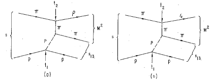
Two-channel Deck amplitudes. We follow closely Refs. Berger:1976nr and Basdevant:1977ya . We consider the Deck amplitudes for production of the quasi-two body systems and at small momentum transfer and high incident energy. We denote these and . The reactions are represented in Figs.1 (a) and (b).
The case has been studied at length. Its amplitude (c.f., Eq. (2.1) of Ref. Basdevant:1977ya ) is
| (1) |
where is the coupling constant (), is the magnitude of the incident pion momentum in the rest frame Berger:1976nr , is the slope of the elastic diffraction peak, and is the total cross-section. The invariants , and are labeled in Fig. 1 (a).
Similarly, the production amplitude is
| (2) |
Choosing the average value of the width of MeV, we obtain a numerical value GeV. The other factors in Eq. (2), relative to Fig. 1 (b) have the same meaning as in Eq. (1).
The Deck background has been well studied, where, by background, we mean the amplitude before any final state interactions are included. We refer to Ref. Basdevant:1977ya and extract what is useful in the present analysis. We work in the final () center of mass frame; is the invariant mass of this system. In the limit of forward production and large , Eq. (1) produces the system predominately in an S-wave Berger:1976nr , used in previous calculations (e.g., Ref. Basdevant:1977ya ).
However, the system is in an orbital P-wave. To address , we must extend the partial wave extraction calculations to finite values of and . We present the complete calculation of these amplitudes elsewhere Basdevant:2015ysa . The important feature is that the higher partial wave amplitudes are of order or with respect to the dominant S-wave. An immediate consequence is that P-wave production should have a noticeably smaller rate than the S-wave process, as is borne out in the complete calculation and exhibited by the COMPASS data, where the intensity of the peak at 1.42 GeV, is lower than that of the peak at 1.26 GeV by a factor of the order of a few .
In the COMPASS experiment, the value of the square of the invariant total energy is GeV2 while the momentum-transfer in the smallest bin is GeV2. We are interested in values of to GeV. Since , the only relevant kinematic corrections come from the momentum transfer dependence. We choose to work at the fixed value GeV2, and we checked that within the first t-bin ( GeV2), our results do not vary appreciably. A convenient dimensionless expansion parameter is
| (3) |
The S-wave background amplitude is, to first order in ,
| (4) | |||||
where and are the pion and energies in the rest frame, and where is the phase space factor, being the pion momentum in the rest frame.
The P-wave amplitude is, at the same order in ,
| (5) | |||||
where , are the pion and energies, the pion momentum in the rest frame and, as above, .
Equation (5) is a major clue to our investigation. The right hand side contains the factor . This factor is negative at low values of (since , but it vanishes near GeV and becomes positive afterward. Furthermore, if we give this term some small imaginary part, its phase will switch suddenly from to zero. This sudden and rapid phase variation is not a dynamical effect in the sense of a resonant phase, but it originates in the structure of the dynamical process by which the state is produced. Another interesting qualitative feature of Eq. (5) is that it grows in the region of interest ( to GeV) and therefore tends to push a resonance peak upward in .
Keeping in mind the parameters introduced in Eqs. (1) and (2), our two amplitudes are
| (6) |
where, and can be read off from Eqs. (4) and (5). The structure remains the same after
we unitarize. The normalization factor is irrelevant for present purposes and is taken equal to here.
Unitarization. For theoretical and technical details about multi-channel final state unitarization, we refer to the literature, in particular to Ref. Babelon:1976kv where the general analysis may be found and to Ref. Basdevant:1977ya where a specific application is made. We recall that if is the (two-channel) strong interaction matrix, then the unitarized Deck amplitude , which we can write as a two dimensional vector as in Eq.(6), has a right hand unitarity cut along which it satisfies the relation
| (7) |
and being the values of the unitarized Deck amplitude above and below the cut.
Our basic assumption is that there is a single resonance whose (unique) second-sheet pole parameters we determine. Since we are dealing with a two-channel case, we parametrize the coupled and final state interactions (or rescattering) via this resonance. In order to do this, we introduce a matrix, as in Eq.(3.14) of Ref. Basdevant:1977ya :
| (8) |
The crucial tool to treat coupled channel final state interactions is a -matrix, related directly to the matrix. It is presented explicitly in Eq.(3.15) of Basdevant:1977ya :
| (9) |
where , and are Chew-Mandelstam functions Chew:1960iv , and the energy denominator function is
| (10) |
The function contains all the information (that we put in) on the coupled-channel - strong interaction. It is an analytic function which possesses the and branch cuts from to infinity and from to infinity. Its second sheet pole determines the nominal position and width of the resonance.
As in Basdevant:1977ya , the unitarized Deck amplitude with resonant rescattering corrections taken into account is
| (11) | |||||
Here is a two-dimensional vector and is the “background” Deck amplitude discussed above.
Direct production contribution. In addition to its manifestation through final state interactions, the may also be produced directly in a diffractive process . For direct production, we choose
| (12) |
where represents the diffractive coupling to the to the , and are the couplings of the in the and channels respectively. Our final amplitude is
| (13) |
In the one-channel case exemplified by photo-production Soding:1965nh , the interference of these two terms can shift the apparent peak position of the .
Analysis and results. Some salient points can be made short of a detailed fit to data. We first select appropriate values of the parameters that provide a good global description. The COMPASS results fix these parameters more stringently than when we dealt only with the S-wave system (and other S-wave channels, such as ). Here, the acceptable mass and width of the , defined by the position of the second sheet pole, turn out to be quite restricted. Our analysis indicates that:
,
.
These values of mass and width correspond to values of the parameters GeV2 and GeV.
The interesting parameter to vary is the ratio in order to find the range of values that produce two peaks with appropriate characteristics: the peak occurs at higher mass than the peak, and the ratio of maximal intensities of these peaks, i.e. /, falls between 1,000 and 500, as indicated by the available data. These requirements lead to negative values of in the range . In other words, the couplings to and to have opposite signs. We choose as our central value .
The next step is to determine the amount of direct production necessary to fix the two peaks, one in , the other in , at their desired positions, i.e. GeV for and GeV for . Values such as and in Eq. (12) ensure good positions for the two peaks, and this situation is stable when one varies the parameter . The ratio of direct production to the background Deck amplitude is consistent with the value we obtained previously Basdevant:1977ya in our analysis of data at much lower energies, with smaller statistics.
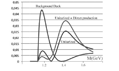
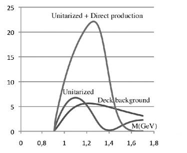
It is interesting to see how the two peaks are built up. We plot in Fig. (2) the shapes of the intensity as a function of the energy , for the various terms in the calculation. The pure Deck background does not produce a resonant shape. The unitarized amplitude shows effectively the zero that appears in the one-channel case Basdevant:1977ya (to which this problem is actually very close). Finally, direct production produces the observed peak, at the right position. A similar set of curves for the intensity is shown in Fig. (3). Notice that the form of the Deck background by itself appears to simulate a narrow resonance peak at threshold (of course without any accompanying phase).
The separation of the positions of the two peaks is evident. The width of is about twice the width of in the calculation. The peak is also more symmetrical, with width about GeV. The lower end of the intensity exhibits a (tiny) peak at around GeV owing to the zero emphasized in Eq. (5).
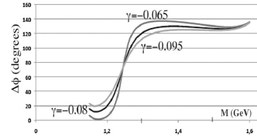
We display in Fig. (4) a set of phase differences between the and amplitudes for three values of our parameter . We adopt as our “central” value (subject to more refined analyses). We call attention to the rapid rise of over in the phase difference in the mass region to GeV. A quantitative fit to the data would yield a precise value of and of the branching ratio of the into of the order of relative to the dominant decay mode .
Summary. We find that the main features of the COMPASS data, two mass peaks separated by MeV with significant relative phase motion, are fully compatible with a single resonance. A detailed quantitative fit of the data with this formalism would lead to a new determination of the mass and width of the and of its branching fraction into .
Acknowledgments. We thank Stephan Paul and other members of the COMPASS collaboration for bringing this interesting topic to our attention. JLB thanks Khosrow Chadan, Philippe Boucaud and Jean-Pierre Leroy, for their considerable help at the Laboratoire de Physique Théorique d’Orsay. ELB is supported in part by the U.S. DOE under Contract No. DE-AC02-06CH11357.
References
- (1) C. Adolph et al. [COMPASS Collaboration], “Observation of a new narrow axial-vector meson ”, arXiv:1501.05732 [hep-ex], submitted to Phys. Rev. Lett.
- (2) K. A. Olive et al. [Particle Data Group Collaboration], Chin. Phys. C 38, 090001 (2014).
- (3) S. D. Drell and K. Hiida, Phys. Rev. Lett. 7, 199 (1961); R. T. Deck, Phys. Rev. Lett. 13, 169 (1964).
- (4) E. L. Berger and J. T. Donohue, Phys. Rev. D 15, 790 (1977); E. L. Berger, J. T. Donohue, and G. Mennessier, Phys. Rev. D 19, 2595 (1979); and references therein.
- (5) J.-L. Basdevant and E. L. Berger, Phys. Rev. D 16, 657 (1977).
- (6) J.-L. Basdevant and E. L. Berger, Phys. Rev. D 19, 246 (1979).
- (7) J.-L. Basdevant and E. L. Berger, Phys. Rev. D 19, 239 (1979).
- (8) J.-L. Basdevant and E. L. Berger, arXiv:1501.04643 [hep-ph].
- (9) O. Babelon, J.-L. Basdevant, D. Caillerie, and G. Mennessier, Nucl. Phys. B 113, 445 (1976), and references therein.
- (10) G. F. Chew and S. Mandelstam, Phys. Rev. 119, 467 (1960); B. W. Lee, Phys. Rev. 120, 325 (1960).
- (11) P. Soding, Phys. Lett. 19, 702 (1966).