Comparing the full time-dependent Bogoliubov–de-Gennes equations to their linear approximation: A numerical investigation

Abstract

In this paper we report on the results of a numerical study of the nonlinear time-dependent Bardeen–Cooper–Schrieffer (BCS) equations, often also denoted as Bogoliubov–de–Gennes (BdG) equations, for a one-dimensional system of fermions with contact interaction. We show that, even above the critical temperature, the full equations and their linear approximation give rise to completely different evolutions. In contrast to its linearization, the full nonlinear equation does not show any diffusive behavior in the order parameter. This means that the order parameter does not follow a Ginzburg–Landau-type of equation, in accordance with a recent theoretical result in FHSchS . We include a full description on the numerical implementation of the partial differential BCS/BdG equations.

1 Introduction

When Bardeen, Cooper and Schrieffer, shortly BCS, published one of the most famous papers in physics in 1957 BCS , giving the first microscopic explanation for superconductivity, a phenomenological theory for the phenomenon had already been around. Systems close to the critical temperature were described with the help of a macroscopic phase-transition parameter introduced by Ginzburg and Landau in 1950 Ginzburg-Landau . Their theory was the first one to allow for the description of the spatial dependence of the superconductivity inside superconducting alloys and the first with which to explain type-II superconductors and the hexogonally shaped penetrations by magnetic flux.

As the Ginzburg–Landau theory yields reliable results on the large scale, soon the question arose as to whether this model can be understood as a macroscopic limit of BCS theory for systems close to the critical temperature. Gorkov gave a positive answer to this question for the stationary case shortly after the publication of BCS, see Gorkov . A rigorous mathematical proof of the convergence was achieved some years ago proveGLst .

But what remains unclear and controversial up to this day, in particular in terms of a rigorous derivation, is the question whether the time evolution of superconducting systems close to the critical temperature are governed by a Ginzburg–Landau type of equation. After first attempts for a derivation of the macroscopic limit had been presented SteSu ; Schmid ; AbrTs , Gorkov and Eliasberg pointed out that a nonlinear equation could only be valid in a gapless regime GorEli . Still, in Cyrot ; Randeriaetal ; Randeria the authors made a case for a time-dependent Ginzburg–Landau equation for superfluid gases at temperatures slightly above the critical one. The argument is based on the assumption that the nonlinear terms in the BCS/BdG equations only lead to small perturbations but do not quantitatively change the system’s behavior. In more detail, this would mean that the projection of the Cooper pair density onto the center of mass direction is governed by a nonlinear dispersive equation. However, it has been argued recently in FHSchS that for a translation invariant homogeneous system close to equilibrium, the full BCS/BdG equations and their linearization do not yield the same behavior at temperatures close to the critical one. In particular, dissipative behavior can only be expected for the linear approximation of the BCS equations but not for the full equations.

With our work, we demonstrate this result by means of a thorough numerical study of the long-term evolution of the BCS equations and their linearization for spatially homogeneous systems close to equilibrium at temperatures slightly above the critical one. For decreasing values of the parameter $h$, defined via $T=(1+h^{2})T_{c}$, we evolve the full and the linear system over a long time span and track the behavior of the Cooper pair density and the order parameter. For each values of the small parameter $h$, we find clear differences between the full equation and its linearization. Additionally, we see that the full BCS /BdG equations yield oscillations in the order parameter about a constant value. Such a behavior has long been predicted for and already been observed in out-of-equilibrium systems, see, e.g., VolkovKogan ; Barankov1 ; Yuzbashyan . Although the focus of our study is not on oscillations in particular but rather on the long-term behavior of the equations in general, it is interesting that we can replicate such oscillations for systems close to equilibrium.

In the realm of numerical analysis, the treatment of quantum dynamical systems has been of huge interest for many decades (see bluebook for an extensive overview). Various evolution schemes for the linear Schrödinger equation in varying settings have been proposed, see, e.g., FeitFleckSteiger ; GrayManolopoulos ; BlanesCasasMurua ; TalEzerKosloff ; ParkLight . Nonlinear Schrödinger equations such as the Gross–Pitaevskii equation and equations arising from the Hartree and Hartree–Fock approximation of the quantum state have also been devoted attention to, see, e.g., Bao ; Thalhammer ; TVZPG ; GaucklerLubich  and LubichMCTDH ; Lubichvar . Regarding the BCS regime, the stationary equations have been treated numerically in LewinPaul and the time-dependent BCS/BdG equations have been considered from an analytical perspective in HLLSch . But, the above-mentioned studies of the out-of-equilibrium dynamics of the BCS equations (VolkovKogan ; Barankov1 ; Yuzbashyan ) notwithstanding, to the best of our knowledge the coupled nonlinear time-dependent BCS equations have not been paid much attention to from a numerical point of view. Therefore, we come up with a reliable integration algorithm for the evolution of the system.

The paper is organized as follows: First, we introduce the system we are considering and the physical background in Section 2. This is followed by a brief summary of the theoretical results of FHSchS in Section 3. Then, we present our numerical results for the linear and the full equation in Section 4. Finally, we summarize our main results in Section 5. A detailed discussion of the initial setup of the system and the numerical implementation is provided in the Appendix Sections A and B, respectively.

2 Physical and mathematical background

2.1 Energy functional and BCS equations

In mathematical terms, BCS theory is a special case of a generalized Hartree–Fock variational principle, itself described by Bogoliubov-theory, for the density operators $\gamma:\mathcal{H}\mapsto\mathcal{H}$ and $\alpha:\mathcal{H}\mapsto\mathcal{H}$ acting on the considered Hilbert space $\mathcal{H}$. Those matrices are put together to form the two-by-two operator-valued matrix

$$\Gamma:=\begin{pmatrix}\gamma&\alpha\\ \overline{\alpha}&1-\gamma\end{pmatrix},$$ (1)

see, e.g., BachLiebSolovej for an introduction. The entries of the matrix can be represented by means of their momentum distribution $\hat{\gamma}(k)=\langle a^{\dagger}_{k}a_{k}\rangle$ and the pair density $\hat{\alpha}(k)=\langle a_{k}a_{-k}\rangle$, determining the Cooper pair wave-function via Fourier transform as $\alpha(x-y)=(2\pi)^{-3/2}\int\hat{\alpha}(k)e^{ik\cdot(x-y)}d^{3}k$. We suppress spin in our notation; the pair density $\hat{\alpha}$ is assumed, for simplicity, to be a spin singlet. For a one-dimensional translation invariant system of fermions at temperature $T$ interacting via a potential $V$, the BCS pressure functional per unit volume is given by

$$\mathcal{F}_{T}(\Gamma)=\int_{\mathbb{R}}(p^{2}-\mu)\hat{\gamma}(p)\mathrm{d}p+\int_{\mathbb{R}}|\alpha(x)|^{2}V(x)\mathrm{d}x-TS(\Gamma),$$ (2)

where the entropy $S$ is defined as

$$S(\Gamma):=-\int_{\mathbb{R}}\operatorname{Tr}_{\mathbb{C}^{2}}\left(\Gamma(p)\log\Gamma(p)\right)\mathrm{d}p.$$ (3)

The evolutions of $\alpha$ and $\gamma$ are given by the time-dependent BCS equations which are also known as Bogoliubov–de–Gennes equations deGennes . In momentum space they can be written conveniently in the self-consistent form

$$\imath\dot{\Gamma}_{t}(p) =[H_{\Gamma_{t}}(p),\Gamma_{t}(p)].$$ (4)

Here, the subscript $t$ indicates the time-dependence and the Hamiltonian $H_{\Gamma_{t}}(p)$ is defined as

$$H_{\Gamma_{t}}(p) =\begin{pmatrix}p^{2}-\mu&2[\hat{V}\ast\hat{\alpha}_{t}](p)\\ 2[\hat{V}\ast\overline{\hat{\alpha}_{t}}](p)&\mu-p^{2}\end{pmatrix},$$ (5)

with $\ast$ denoting the convolution. Calculating the upper-left and upper-right entries of the matrix-valued equation (4), we arrive at the system of coupled nonlinear equations

$$\imath\dot{\hat{\gamma}}_{t}(p) =2\left[(\hat{V}\ast\hat{\alpha}_{t})(p)\overline{\hat{\alpha}_{t}}(p)-\overline{(\hat{V}\ast\hat{\alpha}_{t})}(p)\hat{\alpha}_{t}(p)\right],$$ (6)

$$\imath\dot{\hat{\alpha}}_{t}(p) =2(p^{2}-\mu)\hat{\alpha}_{t}(p)+2(\hat{V}\ast\hat{\alpha}_{t})(p)-4(\hat{V}\ast\hat{\alpha}_{t})(p)\hat{\gamma}_{t}(p).$$ (7)

2.2 Contact interactions

In this paper we concentrate on attractive contact interactions, i.e., potentials of the form

$$V(x)=-a\delta(x),\quad a>0,$$ (8)

which lead to exactly solvable systems in the stationary case. Not only is such a potential the most interesting one from a physical model point-of-view but also does it allow us to implement the terms including a convolution in the equations of motion conveniently as we will illustrate in the numerics Section B.

2.3 Initial values

In this work we consider initial data which, in the stationary case, could be described by the Ginzburg-Landau energy functional for temperatures $T$ close to the critical temperature $T_{c}$, i.e., $T=T_{c}+h^{2}$ for a small parameter $h\in\mathbb{R}$. For temperatures above $T_{c}$, the free energy is minimized by the so-called normal state $\Gamma^{\text{N}}$ for which $\alpha^{\text{N}}=0$, $\gamma^{\text{N}}=\nicefrac{{1}}{{1+\exp(\nicefrac{{(p^{2}-\mu)}}{{T}})}}$. For initial data $\Gamma_{0}$ to be within the range of Ginzburg–Landau, they have to satisfy

$$\mathcal{F}_{T}(\Gamma_{0})-\mathcal{F}_{T}(\Gamma^{\text{N}})\leq\mathcal{O}(h^{4}).$$ (9)

This condition can be complied with by choosing

$$\Gamma_{0}=\frac{1}{1+e^{\nicefrac{{H_{\Delta_{0}}}}{{T}}}}$$ (10)

with

$$H_{\Delta_{0}}=\begin{pmatrix}p^{2}-\mu&-\Delta_{0}\\ -\overline{\Delta_{0}}&\mu-p^{2}\end{pmatrix},$$ (11)

where $\Delta_{0}$ is a small parameter of the order of $h$, see, e.g., proveGLst . Calculating the right-hand side of the matrix equation (10) gives

$$\Gamma_{0}=\begin{pmatrix}\hat{\gamma}_{0}&\hat{\alpha}_{0}\\ \overline{\hat{\alpha}_{0}}&1-\hat{\gamma}_{0}\end{pmatrix}$$ (12)

where $\hat{\gamma}_{0}$ and $\hat{\alpha}_{0}$ take the special form

$$\hat{\gamma}_{0} =\frac{1}{2}-\frac{p^{2}-\mu}{2}\frac{\tanh\left(\frac{\sqrt{(p^{2}-\mu)^{2}+|\Delta|^{2}}}{2T}\right)}{\sqrt{(p^{2}-\mu)^{2}+|\Delta|^{2}}}$$ (13)

$$\hat{\alpha}_{0} =\frac{\Delta_{0}}{2}\frac{\tanh\left(\frac{\sqrt{(p^{2}-\mu)^{2}+|\Delta|^{2}}}{2T}\right)}{\sqrt{(p^{2}-\mu)^{2}+|\Delta|^{2}}}.$$ (14)

In our simulations we choose a temperature which is slightly above the critical temperature for the setting under consideration and set the initial value for the gap parameter $\Delta_{0}$ to a non-vanishing value. We explain how to obtain the critical temperature for our setting and how to find physically reasonable initial values for $\Delta$ in the Appendix Section A.

2.4 Ginzburg–Landau and macroscopic parameter

For the stationary case it is well known that the Ginzburg–Landau theory emerges as the macroscopic limit of the BCS theory. To be more specific, define $\left|\alpha^{\ast}\right>$ as the translation invariant minimizer of the BCS functional which, in case of the contact interaction (8), can be calculated via

$$\hat{\alpha}^{\ast}(p)=\frac{\Delta}{2}\frac{\tanh\left(\frac{\sqrt{(p^{2}-\mu)^{2}+|\Delta|^{2}}}{2T}\right)}{\sqrt{(p^{2}-\mu)^{2}+|\Delta|^{2}}}.$$ (15)

Then, for the Cooper pair density $\left|\alpha\right>$ corresponding to the non-translation invariant minimizer of $\mathcal{F}_{T}$, the quantity

$$\psi:=\frac{1}{h}\left<\alpha^{\ast}|\alpha\right>$$ (16)

is an approximate solution of the stationary Ginzburg–Landau equation, see, e.g., FHSS3 . This told, if there were an analogous relation between the time-dependent BCS and the GL equations, the order parameter

$$\psi_{t}:=\frac{1}{h}\left<\alpha^{\ast}|\alpha_{t}\right>$$ (17)

should, close to $T_{c}$, approximately satisfy a conventional time-dependent Ginzburg–Landau (TDGL) equation. In the spatially homogeneous case we are studying in this work, the conventional TDGL equation takes the form

$$\dot{\psi}_{t}=-c_{\text{GL,1}}\psi_{t}-c_{\text{GL,2}}|\psi_{t}|^{2}\psi_{t},$$ (18)

with some appropriate parameters $c_{\text{GL,1}}$ and $c_{\text{GL,2}}$, see, e.g., Cyrot and (Randeria, , Eq. (18)). The parameter $c_{\text{GL,1}}$ depends on $\nicefrac{{(T-T_{c})}}{{(h^{2}T_{c})}}$. Crucially, $c_{\text{GL,1}}$ has the same sign as $(T-T_{c})$. Thus, the TDGL equation is dissipative for temperatures above $T_{c}$ by definition. This implies that if $\psi_{t}$ could be described by the TDGL for small $h$ it should decay over time. However, we will demonstrate in Section 4 that this is not the case, at least for the full non-linear equation. The same conclusion has been reached by an analytical investigation recently as we will outline in Section 3.

2.5 The linear approximation

Let us decompose the particle density as

$$\gamma_{t}=\gamma_{0}+\eta_{t}.$$ (19)

For states satisfying (9) $\eta_{t}$ appears to depend quadratically on $\hat{\alpha}_{t}$, see, e.g., (FHSchS, , Eq. 11), and it seems legitimate to approximate the full equation by its linearization

$$\imath\dot{\hat{\alpha}}_{t}(p)=2(p^{2}-\mu)\hat{\alpha}_{t}(p)+2(\hat{V}\ast\hat{\alpha}_{t})(p)(1-2\hat{\gamma}_{0}(p)).$$ (20)

However, close to the Fermi-surface the quantity $\eta_{t}$ is not small but the dominant part in the non-linear evolution. Consequently, the full BCS equations (6)-(7) and the linearization (20) give rise to very different evolutions. Namely, Eq. (20) yields a dissipative behavior in $\psi_{t}$ whereas the full equations do not as is shown formally in FHSchS and as we confirm by our numerical experiments below. Let us briefly summarize the results of FHSchS in the next Section.

3 Recent mathematical results

The BCS time-evolution (4) is studied analytically in FHSchS . Based on the work proveGLst the authors prove in (FHSchS, , Theorem 1) that $|\psi_{t}|$ does not vanish for any times. More precisely, it is shown in a very general setting that, if the initial state $\Gamma_{0}$ is close to the energy of the normal state, i.e., $\mathcal{F}_{T}(\Gamma_{0})-\mathcal{F}_{T}(\Gamma^{N})\leq O(h^{4})$, then the corresponding $\psi_{t}$ satisfies

$$||\psi_{t}|-|\psi_{0}||\leq Ch^{1/2},$$ (21)

for an appropriate constant $C$ independent of $h$.

On the other hand, it is shown in FHSchS that the solution of the linearized equation (20) tends to $0$ exponentially fast compared to the system’s time scale of $\nicefrac{{1}}{{h^{2}}}$. In detail, using strategies from perturbation theory, it can be derived that

$$|\psi_{t}|\approx|\psi_{0}|e^{t\operatorname{Im}\lambda}$$ (22)

holds, where $\lambda$ is a resonance of order $\nicefrac{{1}}{{h^{2}}}$ which emerges from the zero-eigenvalue at $T=T_{c}$ of the linear operator $\mathcal{O}=\left(k^{2}-\mu\right)\tanh^{-1}\left(\frac{k^{2}-\mu}{2T}\right)+V$.

The combination of the bounds (21) and (22) shows clearly that the non-dissipative behavior of $\psi_{t}$ is a purely non-linear effect which takes place solely in a tiny neighborhood of the Fermi surface.

Furthermore, using the methods of FHSchS , it is straightforward to derive the following bound on the derivative

$$|\dot{\psi}_{t}|=\mathcal{O}\left(\nicefrac{{1}}{{h}}\right).$$ (23)

In other words, although the solution $|\psi_{t}|$ tends to the constant $|\psi_{0}|$ in the limit $h\to 0$, its derivate might well oscillate more and more –in line with according predictions for systems which are suddenly perturbed out of equilibrium (VolkovKogan ). These findings are well reproduced in our numerical experiments as we show now.

4 Simulations

In this work we are interested in a qualitative study of the differences between the full BCS/BdG equations and their linearization. Thus, without loss of generality, we can work in dimensionless units and set the constant $a$ of the contact interaction and the chemical potential $\mu$ to $a=1$ and $\mu=1$, respectively. The initial data for the simulations are obtained as outlined in the Appendix Section A. For this, we approximate the integrals in Eqs. (25) and (26) by the sum over the discrete momenta we take into account. For the sake of reproducibility we add the thus-obtained values for $T_{c}$ and $\Delta_{0}$ to the results of our simulations. For more details on the discretization of the equations under consideration we refer the interested reader to the Appendix Section B.

4.1 Gap as a function of $h$

In order not to have to calculate the initial value of the gap parameter which depends on the crucial parameter $h$ at the start of each evoluation again, we calculate $\Delta_{0}$ with the procedure outlined in the Appendix Section A for various $h$ once. The interesting result is illustrated in Fig. 1 where we can see that $\Delta_{0}$ depends more or less linearly on the crucial parameter.

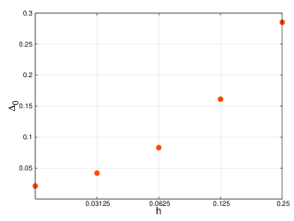
Figure 1: The gap $\Delta_{0}$ as a function of the semiclassical parameter $h$ in semilogarithmic scale.

Finally, with both $T_{c}$ and $\Delta_{0}$ at hand, we are able to present the results of the simulations. Doing so, we take into account that at temperatures $T=T_{c}+h^{2}$, physically interesting dynamics are expected to occur on a time-scale of $\mathcal{O}(\nicefrac{{1}}{{h^{2}}})$. Therefore, we always set $t_{\text{end}}=\nicefrac{{1}}{{h^{2}}}$ or $t_{\text{end}}=\nicefrac{{2}}{{h^{2}}}$ in the following.

4.2 Results for $h=\nicefrac{{1}}{{4}}$

We plot the scaled $L^{2}$-norm of $\alpha$, which in the discrete setting is given by the sum over the $K$ discrete momenta as

$$\frac{1}{h^{2}}\|\alpha_{t}\|^{2}_{2}=\frac{1}{h^{2}}\sum_{k=-\nicefrac{{K}}{{2}}}^{\nicefrac{{K}}{{2}}-1}|\alpha^{K}_{t}(k)|^{2},$$ (24)

as well as the modulus of the interesting macroscopic parameter $\psi_{t}$ introduced in Eq. (17). We plot the results for both the BCS equation (7) and its linear approximation (20), see Fig. 2 and Fig. 3.

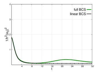
Figure 2: $\nicefrac{{1}}{{h^{2}}}\|\alpha_{t}\|^{2}_{2}$ as a function of integration time $t$ for $h=\nicefrac{{1}}{{4}}$. The physical parameters are $T_{c}=0.19$ and $\Delta_{0}=0.29$.

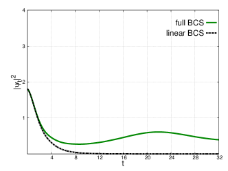
Figure 3: $\psi_{t}$ as a function of integration time $t$ for $h=\nicefrac{{1}}{{4}}$. The physical parameters are $T_{c}=0.19$ and $\Delta_{0}=0.29$.

For both quantities, the linear equation leads to exponential decay. The full equation, in contrast, coincides with the linear approximation only for a short period after which both $\|\alpha_{t}\|$ and $|\psi_{t}|$ grow again.

4.3 Results for $h=\nicefrac{{1}}{{8}}$

Here, too, we consider the scaled norm of the Cooper pair density and the modulus of the parameter $\psi_{t}$. The results are shown in Fig 4 and Fig. 5.

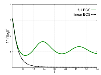
Figure 4: $\nicefrac{{1}}{{h^{2}}}\|\alpha_{t}\|^{2}_{2}$ as a function of integration time $t$ for $h=\nicefrac{{1}}{{8}}$. The physical parameters are $T_{c}=0.19$ and $\Delta_{0}=0.16$.

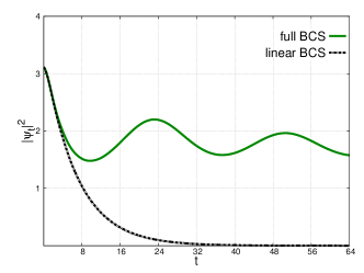
Figure 5: $\psi_{t}$ as a function of integration time $t$ for $h=\nicefrac{{1}}{{8}}$. The physical parameters are $T_{c}=0.19$ and $\Delta_{0}=0.16$.

Again, the linear evolution equation is clearly diffusive while the full equation yields a similar behavior only for very small times. After a short decline in the beginning of the simulation, $\|\alpha_{t}\|$ and $|\psi_{t}|$ seem to oscillate. Similar oscillations have been predicted by VolkovKogan and observed for suddenly perturbed non-equilibrium systems in Yuzbashyan . Although, as compared to these studies, we work on systems close to equilibrium and slightly above the critical temperature, it is interesting to see that our long-term evolutions show oscilllations which resemble the ones predicted for the out-of-equilibrium case.

4.4 Results for $h=\nicefrac{{1}}{{16}}$

Once more, we depict the time evolution of $\|\alpha_{t}\|$ and $|\psi_{t}|$, cf. Figs. 6 and 7.

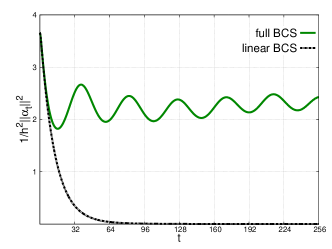
Figure 6: $\nicefrac{{1}}{{h^{2}}}\|\alpha_{t}\|^{2}_{2}$ as a function of integration time $t$ for $h=\nicefrac{{1}}{{16}}$. The physical parameters are $T_{c}=0.19$ and $\Delta_{0}=0.083$.

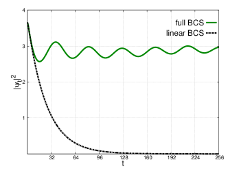
Figure 7: $\psi_{t}$ as a function of integration time $t$ for $h=\nicefrac{{1}}{{16}}$. The physical parameters are $T_{c}=0.19$ and $\Delta_{0}=0.083$.

The conclusions we can draw from these two plots are the same as for $h=\nicefrac{{1}}{{8}}$, the only difference being the faster oscilllations in line with the bound (23). Most importantly, even for this small value of $h$, we only observe diffusion for the linear approximation which, belying its name, does not approximate the BCS equation for reasonably long time intervals. Let us summarize our results in the concluding Section.

5 Summary

We have introduced a reliable integration scheme for the time-dependent BCS equation and its linear approximation in spatially homogeneous settings. With the help of these algorithms, we could perform numerical long-term studies for systems close to equilibrium in order to investigate the time-evolution of the order parameter at the limit close to the critical temperature. The study shows very clearly that, opposed to the linear case, the full BCS equation does not yield any decay over time in the order parameter $\psi_{t}$. Since the conventional time dependent Ginzburg–Landau equation is dissipative above the critical temperature by definition, it cannot give a valid macroscopic limit of the full time-dependent BCS/BdG equations. It can only be seen as the limit of the linearization of the full equations but the effects of this linearization could clearly be shown not to be negligible in the considered regime. We thus confirm the analysis provided in FHSchS .

In addition, when evolving the system as described by the non-linear BCS/BdG equations, we observed oscillations in the Cooper pair density and in the order parameter about a finite value which are similar to oscillations which have been observed for out-of-equilibrium systems in various works.
Acknowledgements: We want to thank Christian Lubich for useful remarks and discussions. This work was partially funded by the DFG grant GRK 1838.
Declaration of contribution Contribution to the original manuscript was: C. H. 30%, J. S. 70%.
Contribution to the update of the manuscript was: C. H. 50%, J. S. 50%.

Appendix A Criticial temperature and initial energy gap

For translation invariant systems with contact interaction, the cricital temperature $T_{c}$ is well-known to be given implicitly by

$$\frac{2\pi}{a}=\int_{\mathbb{R}}\frac{\tanh\left(\frac{p^{2}-\mu}{2T_{c}}\right)}{p^{2}-\mu}\mathrm{d}p,$$ (25)

see, e.g. Leggett ; NRS ; Randeria . The energy gap $\Delta$ between the superconducting state and the normal state at temperatures beneath the cricital temperature, in turn, can be obtained from the relation

$$\frac{2\pi}{a}=\int_{\mathbb{R}}\frac{\tanh\left(\frac{\sqrt{(p^{2}-\mu)^{2}+|\Delta|^{2}}}{2T}\right)}{\sqrt{(p^{2}-\mu)^{2}+|\Delta|^{2}}}\mathrm{d}p.$$ (26)

In order to calculate the critical temperature and a realistic initial value for the gap parameter we thus proceed as follows: For a given value of the small crucial parameter $h$, we first determine the critical temperature $T_{c}$ and set $T=T_{c}-h^{2}$. For this temperature we then search the corresponding gap $\Delta$ following the above definition (26) and set $\Delta_{0}=\Delta$ as its initial state. Finally, as we are interested in simulations for temperatures slightly above the critical temperature, we put $T=T_{c}+h^{2}$ and insert this into Eq. (12) together with the just-determined $\Delta_{0}$. This yields physically realistic conditions which satisfy the energy constraint (9).

Appendix B Numerical treatment of the equations

We want to model a system of infinite spacial extension, which, of course, is not possible to achieve on a machine. Therefore, we pretend our system to be periodic in space but with a large enough period.

B.1 Finite extension and discrete system

In the Ginzburg-Landau regime, one often takes into account external potentials that vary on a scale of $\mathcal{O}(\nicefrac{{1}}{{h}})$ and, consequently, lead to variations of the system which occur over intervals of that very scale. Thus, a valid model system should have an extension no smaller than those physical variations. But, in order to avoid artificial effects due to the periodicity, it is necessary to enlarge this extensions by some multiples of $\nicefrac{{1}}{{h}}$. For convenience we furthermore include a factor of $2\pi$, wherefore we consider systems with period $\nicefrac{{2\pi N}}{{h}}$, $1<N\in\mathbb{N}$. The kernels of the density operators are now functions on $L^{2}([0,\nicefrac{{2\pi N}}{{h}}]\mapsto\mathbb{R})$. In order to simplify the notation, we introduce macroscopic variables via $x_{\text{mac}}:=\nicefrac{{h}}{{N}}x$. We end up in a $2\pi$-periodic setting for which the inner product of two functions $f$ and $g$ is just

$$\left<f|g\right> =\sum_{k\in\mathbb{Z}}\overline{\hat{f}}\hat{g}.$$ (27)

The self-consistent BCS equations are now given by

$$\imath\dot{\Gamma}_{t}(k) =[H_{\Gamma_{t}(K)},\Gamma_{t}(k)],\quad k\in\mathbb{Z},$$ (28)

with the Hamiltonian

$$H_{\Gamma_{t}} =\begin{pmatrix}\left(\frac{h^{2}}{N^{2}}k^{2}-\mu\right)&2[\hat{V}_{Nh}\ast\hat{\alpha}_{t}]_{k}\\ 2[\hat{V}_{Nh}\ast\overline{\hat{\alpha}_{t}}]_{k}&\left(\mu-\frac{h^{2}}{N^{2}}k^{2}\right)\end{pmatrix}$$ (29)

and the Fourier transform $\hat{V}_{Nh}$ of $V_{Nh}(\cdot):=V\left(\nicefrac{{N}}{{h}}\cdot\right)$. Please note that in the present discrete case the convolution of two summable series $a_{k}$ and $b_{k}$ has to be understood as

$$(a\ast b)_{k}=\sum_{j\in\mathbb{Z}}a_{k-j}b_{j}.$$ (30)

B.2 The equations for a delta potential

For systems on a large torus with a contact interaction (8), we can easily see that

$$\hat{V}_{Nh}\ast\hat{\alpha}_{t}=-a\left<\phi|\alpha\right>,$$ (31)

where $\phi$ is the state given by $\phi(k)=1$ for all integers $k$. With this, the equations of motion take the convenient form

$$\imath\dot{\hat{\gamma}}_{t}(k) =2a\left[\overline{\left<\phi|\alpha\right>}\hat{\alpha}_{t}(k)-\left<\phi|\alpha\right>\overline{\hat{\alpha}_{t}}(k)\right],$$ (32)

$$\imath\dot{\hat{\alpha}}_{t}(k) =2\left(\frac{h^{2}}{N^{2}}k^{2}-\mu\right)\hat{\alpha}_{t}(k)+2a\left<\phi|\alpha\right>\left(2\hat{\gamma}_{t}(k)-1\right)$$ (33)

for the nonlinear case and

$$\imath\dot{\hat{\alpha}}_{t}(k) =2\left(\frac{h^{2}}{N^{2}}k^{2}-\mu\right)\hat{\alpha}_{t}(k)+2a\left<\phi|\alpha\right>\left(2\hat{\gamma}_{0}(k)-1\right)$$ (34)

for the linear case.

Up to now we are still left with an infinite-dimensional system of equations. In order to solve these numerically, we have to introduce a suitable finite-dimensional subspace.

B.3 Space discretization

As the BCS equations are given in their momentum space representation, it is most convenient to use the so-called Fourier collocation. This means that a $2\pi$-periodic function $f(x)=\sum_{j\in\mathbb{Z}}\hat{f}(j)e^{\imath kx}$ is approximated by

$$f^{K}(x)=\sum_{j=-\frac{K}{2}}^{\frac{K}{2}-1}\hat{f}^{K}(j)e^{\imath kx},$$ (35)

where the coefficients $\hat{f}^{K}(j)$ are obtained by the discrete Fourier transform of the values $f_{j}=f\left(\nicefrac{{2\pi}}{{K}}j\right)$, $j=-\nicefrac{{K}}{{2}},...,\nicefrac{{K}}{{2}}-1$. Mathematically speaking we work on the subspace spanned by the first $K$ eigenfunctions of the Laplacian on $[0,2\pi]$. As a consequence, the evolution of the system is given by the $K$-dimensional system of ordinary differential equations (ODE)

$$\imath\dot{\hat{\gamma}}^{K}_{t}(k)=2a\left[\overline{\left<\phi^{K}|\alpha^{K}\right>}\hat{\alpha}^{K}_{t}(k)-\left<\phi^{K}|\alpha^{K}\right>\overline{\hat{\alpha}^{K}_{t}}(k)\right],$$ (36)

$$\quad\quad-\frac{K}{2}\leq k\leq\frac{K}{2}-1,$$

$$\imath\dot{\hat{\alpha}}^{K}_{t}(k)=2\left(\frac{h^{2}}{N^{2}}k^{2}-\mu\right)\hat{\alpha}^{K}_{t}(k)$$

$$\phantom{\imath\dot{\hat{\alpha}}^{K}_{t}(k)=}+2a\left<\phi^{K}|\alpha^{K}\right>\left(2\hat{\gamma}^{K}_{t}(k)-1\right),$$ (37)

$$\quad\quad-\frac{K}{2}\leq k\leq\frac{K}{2}-1,$$

and accordingly for the linear case. From numerical analysis it is well known that (35) yields a very good approximation to $2\pi$-periodic functions with the discretization error decreasing rapidly as a function of $K$, see, e.g. bluebook , Chapter III.1.3.

For practical reasons we set $K$ to be an integer power of $2$ so that for a given $\hat{\alpha}^{K}_{t}(j)$, $j=-\nicefrac{{K}}{{2}},...,\nicefrac{{K}}{{2}}-1$, the corresponding distribution $\alpha^{K}_{t}(x)$ at the discrete points $x_{j}=\frac{2\pi}{K}j$ can be computed efficiently with the well-known fast Fourier transform (FFT). As we want to resolve phenomena happening on the microscopic scale $\mathcal{O}(\nicefrac{{h}}{{N}})$, we choose

$$K=M\frac{N}{h}$$ (38)

for a large enough integer $M$. Let us now explain how we solve the system of ODE (36)–(37).

B.4 Solving the system of ordinary differential equations

We first notice that the Hamiltonian $H_{\Gamma_{t}}$ is self-adjoint. Thus, the time-evolution of $\Gamma_{t}$ is a unitary transformation and, hence, its eigenvalues are preserved. With regard to definition (1), the eigenvalues can be readily computed as

$$\lambda_{1,2}(p) =\frac{1}{2}\pm\sqrt{\left(\hat{\gamma}_{t}(p)-\frac{1}{2}\right)^{2}+|\hat{\alpha}_{t}(p)|^{2}},$$ (39)

and we see that the equality

$$\left(\hat{\gamma}_{t}(p)-\frac{1}{2}\right)^{2}+|\hat{\alpha}_{t}(p)|^{2} =\left(\hat{\gamma}_{0}(p)-\frac{1}{2}\right)^{2}+|\hat{\alpha}_{0}(p)|^{2}$$ (40)

holds. Solving this for $\hat{\gamma}_{t}$, we get

$$\hat{\gamma}_{t}(p) =\begin{cases}\frac{1}{2}+\sqrt{h(p)-|\hat{\alpha}_{t}(p)|^{2}}\text{ for $p^{2}<\mu$,}\\ \frac{1}{2}-\sqrt{h(p)-|\hat{\alpha}_{t}(p)|^{2}}\text{ for $p^{2}\geq\mu$,}\end{cases}$$ (41)

where we have defined the auxiliary function

$$h(p) :=\left(\hat{\gamma}_{0}(p)-\frac{1}{2}\right)^{2}+|\hat{\alpha}_{0}(p)|^{2}.$$ (42)

The signs in Eq. (41) can be inferred from the initial values we use in this work, cf. (12). They are such that $\hat{\gamma}_{0}(p)$ is greater than $\nicefrac{{1}}{{2}}$ for $\mu>p^{2}$ and less than or equal to $\nicefrac{{1}}{{2}}$ for $\mu\leq p^{2}$.

Inserting the discrete analogon of Eq. (41) into the relevant equation of motion (37), we get the nonlinear coupled system of equations

$$\imath\dot{\hat{\alpha}}^{K}_{t}(k) =2\left(\frac{h^{2}}{N^{2}}k^{2}-\mu\right)\hat{\alpha}^{K}_{t}(k)$$

$$\phantom{=}\pm 4a\left<\phi^{K}|\alpha^{K}\right>\sqrt{h(k)-|\hat{\alpha}^{K}_{t}(k)|^{2}},-\frac{K}{2}\leq k\leq\frac{K}{2}-1.$$ (43)

This said, we now present our time integration algorithm.

B.5 Time discretization

Putting it in a formal way, the system we have to integrate is given by

$$\begin{cases}\frac{\mathrm{d}\mathbf{y}(t)}{\mathrm{d}t}&=f(\mathbf{y}(t)),\\ \mathbf{y}(0)&=\mathbf{y}_{0},\end{cases}$$ (44)

with

$$\mathbf{y}=\begin{pmatrix}\hat{\alpha}^{K}\left(-\nicefrac{{K}}{{2}}\right)&\ldots&\hat{\alpha}^{K}\left(\nicefrac{{K}}{{2}}-1\right)\end{pmatrix}^{T}\in\mathbb{R}^{K}.$$ (45)

The right hand side of our initial problem can be written as the sum of two terms,

$$f(\mathbf{y})=f_{1}(\mathbf{y})+f_{2}(\mathbf{y}),$$ (46)

where $f_{1}$ represents the linear part which resembles the kinetic part in the Schrödinger-equation and $f_{2}$ is the nonlinear part. Let $\tau$ denote a time step and $\Phi_{\tau,f}$ the smooth map between $\mathbf{y}(0)$ and $\mathbf{y}(\tau)$. Given the special form (46) of the differential equation, one can approximate $\Phi_{\tau,f}$ numerically by

$$\Phi^{\text{num}}_{\tau,f}(\mathbf{y}_{0})=\left(\Phi_{\nicefrac{{\tau}}{{2}},f_{1}}\circ\Phi_{\tau,f_{2}}\circ\Phi_{\nicefrac{{\tau}}{{2}},f_{1}}\right)(\mathbf{y}_{0}).$$ (47)

This is the well-known Strang splitting. Applying it successively yields an approximation to the exact solution at times $t=n\tau$, $n=1,2,...$, the error of which decreases quadratically as a function of the step size $\tau$, see, e.g. hairerlubichwanner , Chapter II.5.

The advantage of the Strang splitting is that $\Phi_{\tau,h}$ can be calculated exactly as

$$\Phi_{\tau,f_{1}}(\cdot)=e^{-\imath 2\left(\frac{h^{2}}{N^{2}}k^{2}-\mu\right)\tau}\cdot.$$ (48)

As for $\Phi_{\tau,f_{2}}$, it has to be approximated due to the nonlinearity. For this, we choose a simple Runge-Kutta scheme as proposed by nr whose numerical error is small compared to the error expacted from the splitting remark . Before starting the simulations, we still need to fix the mentioned discretization parameters $\tau$ and $K$. In our case, $K$ itself depends on three parameters, cf. Eq. (38). As $h$ is the semiclassical parameter we want to vary throughout the study, we have to choose reasonable values for the remaining quantities $M$, $N$ and $\tau$. We first consider $\tau$.

B.6 Fixing the time discretization parameter

The step size has to be chosen small enough for both the numerical approximation of $\Phi_{\tau,f_{2}}$ and the Strang splitting to give accurate results. For our simulations it turned out that reliable results can only be expacted for a step size inversely proportional to $K$. Playing safe we include a small factor and set $\tau=\nicefrac{{0.1}}{{K}}$. As a measure for the time integrator’s accuracy, we consider the discrete analogon of the free energy introduced in Eq. (2) above, which is given by

$$F_{T}^{K}(\Gamma^{K}) =\sum_{k=-\nicefrac{{K}}{{2}}}^{\nicefrac{{K}}{{2}}-1}\left(\frac{h^{2}}{N^{2}}k^{2}-\mu\right)\hat{\gamma}^{K}(k)$$

$$\phantom{=}+\frac{1}{2\pi}\int_{0}^{2\pi}V(x_{\text{mac}})|\alpha^{K}(x_{\text{mac}})|^{2}\mathrm{d}x_{\text{mac}}-TS(\Gamma^{K}).$$ (49)

A short calculation yields that this quantity is conserved under the exact flow of the corresponding initial value problem. Therefore, the reliability of a numerical integration scheme can be checked by tracking the relative error $\Delta F_{T}$, defined by

$$\Delta F_{T}(t)=\left|\frac{F_{T}(\Gamma^{K}_{t})-F_{T}(\Gamma^{K}_{0})}{F_{T}(\Gamma^{K}_{0})}\right|,$$ (50)

along the numerical evolution. Recurring to a constant of motion as a criterion of accurateness is a much applied procedure in various computational fields, see, e.g. Seyrich ; Lukes . Following this line of reasoning, we have verified the accuracy of our time integrator for every simulation presented below. As an example, we show the plot of $\Delta F_{T}$ corresponding to the simulations of Subsection 4.3 in Fig. 8.

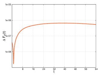
Figure 8: Relative error $\Delta F_{T}$ of the discretized free energy against integration time $t$ in semilogarithmic scale for $h=\nicefrac{{1}}{{8}}$. The physical parameters are $T_{c}=0.19$ and $\Delta_{0}=0.16$.

B.7 Fixing the space discretization parameters

We have seen in the previous Subsection that the time step has to be inversely proportional to the dimension of the subspace we are approximating our system on. Furthermore, every time step requires a computational effort which grows linearly with $K$. Consequently, the complete CPU time for a simulation over a given time interval $[0,t_{\text{end}}]$ is quadratic in $K$. So the dimension of the subspace and, thus, the related $N$ and $M$ should be the smallest possible. In order to check how small a $M$ we can choose without any significant loss of accuracy, we fix $N=8$ and $h=\nicefrac{{1}}{{4}}$ and calculate the cricital temperature via the discretized version of Eq. (25),

$$\frac{2\pi}{a}=\sum_{k=-\nicefrac{{K}}{{2}}}^{\nicefrac{{K}}{{2}}-1}\frac{\tanh\left(\frac{\frac{h^{2}}{N^{2}}k^{2}-\mu}{2T_{c}}\right)}{\frac{h^{2}}{N^{2}}k^{2}-\mu},$$ (51)

for different values of $M$. The result can be seen in Fig. 9.

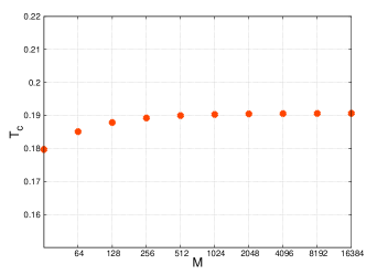
Figure 9: Critical temperature $T_{c}$ as a function of the number of momenta per unit volume $M$ for $N=8$ and $h=\nicefrac{{1}}{{4}}$.

For different values of $N$ and $h$ we get the same plot. We see that for $M=256$ the critical temperature is still slightly too small. However, when comparing the evolutions obtained with $M=256$ to the according ones for $M=512$, the relevant figures are indistinguighable from each another. For the sake of efficiency, we thus fix $M=256$ for the rest of this work.

As for the extension of our interval, $N$, we have to choose it large enough so that the solution cannot reach the boundaries during the simulation. As, by construction, we work with a periodic setting, a solution reaching one end of the interval would enter again at the other end, thus leading to unphysical interference. As an example of this numerical artifact, we consider the case $h=\nicefrac{{1}}{{8}}$, $N=4$ and plot the modulus of $\psi_{t}$ in Fig. 10.

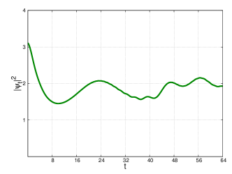
Figure 10: $\psi_{t}$ as a function of integration time $t$ for $N=4$ and $h=\nicefrac{{1}}{{8}}$. The physical parameters are $T_{c}=0.19$ and $\Delta_{0}=0.16$.

We observe oscillations for larger $t$ which should not show up in reality, cf. Subsection 4.3. Whenever we encountered such an artifact, we successively increased $N$ by factors of $2$ until the artifact vanished.

References

- (1) R. L. Frank, C. Hainzl, B. Schlein, R. Seiringer, preprint, arXiv:1504.05885
- (2) J. Bardeen, L. N. Cooper and J. R. Schrieffer, Physical Review 108, 1175 (1957)
- (3) E. P. Gross, Il Nuovo Cimento 10, 454 (1961)
- (4) L. P. Pitaevskii, Sov. Phys. JETP 13, 451 (1961)
- (5) L. D. Landau and V. L. Ginzburg, Zh. Eksp. Teor. Fiz. 20, 1064 (1950)
- (6) L. P. Gorkov, Sov. Phys. JETP 9, 1364 (1959)
- (7) R. L. Frank, C. Hainzl, R. Seiringer and J. P. Solovej, J. Amer. Math. Soc. 25, 667 (2012)
- (8) A. J. Leggett, Lecture Notes in Physics, vol. 115 (Springer, Berlin, 1980) pp. 13-27
- (9) P. Noziéres and S. Schmitt-Rink. Journal of Low Temperature Physics, 59:195–211, 1985.
- (10) M. Drechsler and W. Zwerger, Ann. Phys. 504, 15 (1992).
- (11) C. Hainzl and R. Seiringer, Lett. Math. Phys. 100, 119 (2012)
- (12) C. Hainzl and B. Schlein, Journal of Functional Analysis 265, 399 (2013)
- (13) P. Pieri and G.C. Strinati, Phys. Rev. Lett. 91, 030401 (2003)
- (14) M. J. Stephen and H. Suhl, Phys. Rev. Lett. 13, 797 (1964)
- (15) A. Schmid, Z. Phys. 216, 336 (1966)
- (16) E. Abrahams and T. Tsuneto, Phys. Rev. 152, 416 (1966)
- (17) L. P. Gorkov and G. M. Eliasberg, Sov. Phys. JETP 27, 328 (1968)
- (18) M. Cyrot, Rep. Prog. Phys. 36, 103 (1973)
- (19) C. A. R. Sá de Melo, M. Randeria and J. R. Engelbrecht, Phys. Rev. Lett. 71, 3202 (1993)
- (20) M. Randeria, Bose-Einstein Condensation, eds. A. Griffin, D. W. Snoke and S. Stringari (Cambridge University Press, July 1996), pp. 355–392.
- (21) C. Lubich, From Quantum to Classical Molecular Dynamics: Reduced Models and Numerical Analysis (Europ. Math. Soc., Zürich, 2008)
- (22) M. D. Feit, J. A. Fleck Jr. and A. Steiger, J. Comput. Phys. 47, 412 (1982)
- (23) S. K. Gray and D. E. Manolopoulos, J. Comput. Phys. 104, 7099 (1996)
- (24) S. Blanes, F. Casas and A. Murua, J. Comput. Phys. 124, 234105 (2006)
- (25) H. Tal-Ezer and R. Kosloff, J. Chem. Phys. 81, 3967 (1984)
- (26) T. J. Park, J. Chem. Phys. 85, 5870 (1986)
- (27) W. Bao, D. Jaksch and P. A. Markowich, J. Comput. Phys. 187, 318 (2003)
- (28) M. Caliari, C. Neuhauser and M. Thalhammer, J. Comput. Phys. 228, 822 (2009)
- (29) L. Gauckler and C. Lubich, Found. Comput. Math. 10, 275 (2010)
- (30) Y.-F. Tang, L. Vázquez, F. Zhang and V. M. Pérez-García, Computers Math. Applic. 32, 73 (1996)
- (31) C. Lubich, Appl. Numer. Math. 48, 355 (2004)
- (32) C. Lubich, Math. Comp. 74, 765 (2005)
- (33) M. Léwin and S. Paul, ESAIM: Mathematical Modelling and Numerical Analysis 48, 53 (2014)
- (34) C. Hainzl, E. Lenzmann, M. Léwin and B. Schlein, Ann. H. Poincaré 11, 1023 (2010)
- (35) A. . Volkov and S. M. Kogan, Sov. Phys. JETP 38, 1018 (1974)
- (36) R. A. Barankov, L. S. Levitov and B. Z. Spivak, Phys. Rev. Lett. 93, 160401 (2004)
- (37) E. A. Yuzbashyan, O. Tsyplyatyev and B. L. Altshuler, Phys. Rev. Lett. 96, 097005 (2006)
- (38) V. Bach, E. H. Lieb and J. P. Solovej, Journal of statistical physics 76, 3 (1994)
- (39) P. G. de Gennes and P. A. Pincus Superconductivity of metals and alloys (WA Benjamin, New York, 1966), Vol. 86.
- (40) C. Hainzl, E. Hamza, R. Seiringer and J. P. Solovej, Comm. Math. Phys 281, 349 (2008)
- (41) R.L. Frank, C. Hainzl, R. Seiringer, J.P. Solovej, Operator Theory: Advances and Applications Volume 227, 57–88 (2013),
- (42) E. Hairer, C. Lubich and G. Wanner, Geometric numerical integration. Structure-preserving algorithms for ordinary differential equations (Springer, Berlin, 2006), 2nd ed.
- (43) W. Press, S. Teukolsky, W. Vetterling and B. Flannery, Numerical Recipes in C. The art of scientific computing (Cambridge University Press, 1992), 2nd ed.
- (44) J. Seyrich, Phys. Rev. D 87, 084064 (2013)
- (45) G. Lukes-Gerakopoulos, Phys. Rev. D 89, 043002 (2014)
- (46) Note that in the linear case can also be calculated exactly.