Symmetry reduction in high dimensions, illustrated in a turbulent pipe

Abstract

Equilibrium solutions are believed to structure the pathways for ergodic trajectories in a dynamical system. However, equilibria are atypical for systems with continuous symmetries, i.e. for systems with homogeneous spatial dimensions, whereas relative equilibria (traveling waves) are generic. In order to visualize the unstable manifolds of such solutions, a practical symmetry reduction method is required that converts relative equilibria into equilibria, and relative periodic orbits into periodic orbits. In this article we extend the fixed Fourier mode slice approach, previously applied 1-dimensional PDEs, to a spatially 3-dimensional fluid flow, and show that is substantially more effective than our previous approach to slicing. Application of this method to a minimal flow unit pipe leads to the discovery of many relative periodic orbits that appear to fill out the turbulent regions of state space. We further demonstrate the value of this approach to symmetry reduction through projections (projections only possible in the symmetry-reduced space) that reveal the interrelations between these relative periodic orbits and the ways in which they shape the geometry of the turbulent attractor.

Chaotic dynamics can be interpreted as a trajectory in state space, where each coordinate corresponds to a degree of freedom. For higher-dimensional systems it can be difficult to predict which coordinate choices will provide the most instructive projections, given that plots of these trajectories are limited to displaying two or three dimensions at a time. To avoid clutter in the projection caused by families of orbits related by translations or reflections, symmetry-invariant measures such as spatial averages are often favored. In practice, however, there are only so many quantities that may be averaged and, in addition, information held in the spatial structure is wiped out in the averaging process. Often such averaging results in a largely uninformative projection of the dynamics.

The study of turbulence is one example where substantial progress has recently been made by viewing the flow as a dynamical system, but now a more informative means of projection is required to comprehend the way in which the unstable manifolds of relative equilibria and other invariant solutions shape the dynamics. These invariant solutions correspond to recurrent but unstable motions Hof et al. (2004) that share some characteristics with fully turbulent flows. Experiments Hof et al. (2004); Dennis and Sogaro (2014) and simulations Kerswell and Tutty (2007); de Lozar et al. (2012) have identified transient visits to spatiotemporal patterns that mimic traveling wave solutions. Certain low-dissipation traveling waves of the Navier-Stokes equations have been shown to be important in the transition to turbulence, where they lie in the laminar-turbulent boundary, separating initial conditions that ultimately relaminarize from those that develop into turbulence Duguet et al. (2008). Spatiotemporal flow patterns called ‘puffs’ and ‘slugs’ are observed during the evolution to turbulence. Recently, spatially-localized solutions representative of puffs have been discovered Avila et al. (2013) and shown to be linked to spatially-periodic traveling waves in minimal domains Chantry et al. (2014). As traveling waves are steady in their respective co-moving frames, they are relative equilibria, solutions that do not exhibit temporal shape-changing dynamics. Their unstable manifolds, however, mold the surrounding state space, carving pathways for relative periodic orbits, invariant orbits embedded in turbulence whose temporal evolution captures dynamics of ergodic trajectories that shadow them. A detailed understanding of these recurrent motions is crucial if one is to systematically describe the repertoire of all turbulent motions. With the removal of spatial translations, which obscure visualizations of the dynamics, a far greater number of projections of chaotic trajectories is possible. In this article, we show that visualizations of the symmetry reduced dynamics can help us understand relationships between distinct families of periodic orbits and traveling wave solutions, which in turn lends support to the dynamical systems interpretation that relative periodic orbits form the backbone of turbulence in pipe.

Our approach is dynamical: writing the Navier–Stokes equations as $\dot{\mbox{\boldmath$u$}}=\mbox{\boldmath$v$}(\mbox{\boldmath$u$})$, the fluid state $u$ at a particular moment in time is represented by a single point in state space ${\cal M}$ Gibson et al. (2008); turbulent flow is represented by an ergodic trajectory that wanders between accessible states in ${\cal M}$ Hopf (1948). Essential to this analysis is that any two physically equivalent states be identified as a single state: a symmetry-reduced state space $\hat{\cal M}={\cal M}/G$ is formed by contracting the volume of state space representing states that are identical except for a symmetry transformation to a single point $\hat{\mbox{\boldmath$u$}}$. Only after a symmetry reduction are the relationships between physically distinct states revealed. In this article symmetry reduction is implemented with an extension of the ‘first Fourier mode slice’ method Budanur et al. (2015), a variant of the method of slices Cartan (1935). The method of slices separates coordinates into phases along symmetry directions (‘fibers’, ‘group orbits’ that parametrize families of physically-equivalent dynamical states) from the remaining coordinates of the symmetry-reduced state space $\hat{\cal M}$. The latter capture the dynamical degrees of freedom—those associated with structural changes of the flow.

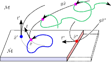
Figure 1: (Color online) Schematic of symmetry reduction by the method of slices. The blue point is the template ${\hat{x}^{\prime}}$. Group orbits are marked by dotted curves, so that all pink points are equivalent to $\hat{x}$ up to a shift. The relative periodic orbit (green) in the $d$-dimensional full state space ${\cal M}$ closes into a periodic orbit (blue) in the slice $\hat{\cal M}={\cal M}/G$, a $(d\!-\!1)$-dimensional slab transverse to the template group tangent $t^{\prime}$. A typical group orbit crosses the slice hyperplane transversally, with a non-orthogonal group tangent $t=t(\hat{x})$. A slice hyperplane is almost never a global slice; it is valid up to the slice border, a $(d\!-\!2)$-dimensional hypersurface (red) of points $\hat{x}^{\ast}$ whose group orbits graze the slice, i.e. points whose tangents $t^{*}=t(\hat{x}^{\ast})$ lie in $\hat{\cal M}$. Beyond the slice border (dashed ‘chunk’), group orbits do not cross the slice hyperplane locally.

The Navier-Stokes equations are invariant under translations, rotations, and inversions about the origin, and the application of any of these symmetry operations to a state $\mbox{\boldmath$u$}(\mbox{\boldmath$x$})$ results in another dynamically equivalent state. The boundary conditions for pipe flow restrict symmetries to translations along the axial and azimuthal directions, and reflections in the azimuthal direction. In the computations presented here,axial periodicity is assumed so that the symmetry group of the system is $O(2)_{\theta}\times SO(2)_{z}$. In order to illustrate the key ideas, we constrain azimuthal shifts, and focus on the family of streamwise translational shifts $\{g\}$ parametrized by a single continuous phase parameter $\ell$,

$$(g(\ell)\,\mbox{\boldmath$u$})(z)=\mbox{\boldmath$u$}(z-\ell)\,.$$

If periodic axial symmetry is assumed, application of $g$ gives a closed curve family of dynamically equivalent states — topologically a circle, called a group orbit — in state space ${\cal M}$. Were azimuthal (‘spanwise’) shifts included, equivalent states would lie on a 2-torus.

Symmetry reduction simplifies the state space by reducing each set of dynamically equivalent states to a unique point $\hat{\mbox{\boldmath$u$}}$. The method of slices achieves this with the aid of a fixed template state $\mbox{\boldmath$u$}^{\prime}$ (see Fig. 1). A shift is applied so that the symmetry-reduced state $\hat{\mbox{\boldmath$u$}}=g(-\ell)\mbox{\boldmath$u$}$ lies within the hyperplane orthogonal to $\mbox{\boldmath$t$}^{\prime}=\lim_{\ell\to 0}\,(g(\ell)\mbox{\boldmath$u$}^{\prime}-\mbox{\boldmath$u$}^{\prime})/\ell$, the tangent to the template $\mbox{\boldmath$u$}^{\prime}$ in the direction of the shift. For a time-dependent flow, one determines $\ell=\ell(t)$ by chosing $\hat{\mbox{\boldmath$u$}}$ to be the point on the group orbit of $u$ closest to the template, $\langle\hat{\mbox{\boldmath$u$}}-\mbox{\boldmath$u$}^{\prime}|\mbox{\boldmath$t$}^{\prime}\rangle=0$ in a given norm. In this work we use the L2 or ‘energy’ norm $E=\langle\mbox{\boldmath$u$}|\mbox{\boldmath$u$}\rangle/2=\int\mbox{\boldmath$u$}^{2}/2\,dV$.

As traveling waves drift downstream without changing their spatial structure, the family of traveling wave states $\mbox{\boldmath$u$}(t)$ is dynamically equivalent (lies on the same group orbit $g(\ell)\,\mbox{\boldmath$u$}$) and may be represented by a single state $\hat{\mbox{\boldmath$u$}}_{q}$. Thus all traveling waves are simultaneously reduced to equilibria in the slice, irrespective of their individual phase velocities, a powerful property of the method of slices. Furthermore, all relative periodic orbits $p$, flow patterns each of which recurs after a different time period ${T_{p}}$, shifted downstream by a different $\ell_{p}$, close into periodic orbits in the slice hyperplane.

Dynamics within the slice is given by

$$\dot{\hat{\mbox{\boldmath$u$}}} = \mbox{\boldmath$v$}(\hat{\mbox{\boldmath$u$}})-\dot{\ell}(\hat{\mbox{\boldmath$u$}})\,\mbox{\boldmath$t$}(\hat{\mbox{\boldmath$u$}})\,,$$ (1)

$$\dot{\ell}(\hat{\mbox{\boldmath$u$}}) = \langle\mbox{\boldmath$v$}(\hat{\mbox{\boldmath$u$}})|\mbox{\boldmath$t$}^{\prime}\rangle\,/\,\langle\mbox{\boldmath$t$}(\hat{\mbox{\boldmath$u$}})|\mbox{\boldmath$t$}^{\prime}\rangle\,,$$ (2)

where the expression for the phase velocity $\dot{\ell}$ is known as the reconstruction equation Rowley and Marsden (2000). No dynamical information is lost and we may return to the full space by integrating (2). In contrast to a Poincaré section, where trajectories pierce the section hyperplane, time evolution traces out a continuous trajectory within the slice. In principle, the choice of template is arbitrary; in practice, some templates are preferable to others. While one is concerned with the dynamics within the slice $\hat{\mbox{\boldmath$u$}}(t)$, in practice it may be simpler to record $\ell(t)$ and to post-process, or to process on the side, visualizations within the slice—slicing is much cheaper to perform than gathering $\mbox{\boldmath$u$}(t)$ from simulation or laboratory experiment.

The enduring difficulty with symmetry reduction is in determining a unique shift $\ell$ for a given state $u$, while avoiding discontinuities in $\ell(t)$ that arise when multiple ‘best fit’ candidates $\hat{\mbox{\boldmath$u$}}=g(-\ell)\mbox{\boldmath$u$}$ to the template $\mbox{\boldmath$u$}^{\prime}$ occur. A singularity arises if the group orbit $g\mbox{\boldmath$u$}$ grazes the slice hyperplane (Fig. 1). At the instant this occurs, the tangents to the fluid state $\hat{\mbox{\boldmath$u$}}$ and the template $\mbox{\boldmath$u$}^{\prime}$ are orthogonal, and there is a division by zero in the reconstruction equation (2). In ref. Willis et al. (2013) it was shown that the hyperplanes defined by multiple templates could be used to tile a slice, but while switching may permit the symmetry reduction of longer trajectories, it is often not possible to both switch templates before a slice border is reached and to simultaneously maintain continuity in $\ell$. Furthermore, it is uncertain when to switch back to the first template, in order to produce a unique symmetry-reduced state. Our aim in this article is to avoid such difficulties through the use of a single template with distant slice borders. The approach of Budanur et al. Budanur et al. (2015) for the case of one translational spatial dimension fixes the phase of a single Fourier coefficient. This ‘Fourier’ slice is a special case within the slicing framework, with the effect of extreme smoothing of the group orbit. Here the approach is extended to a spatially 3-dimensional case, that of turbulent pipe flow.

For the case of a scalar field defined on one spatial dimension Budanur et al. (2015) there is a unique Fourier coefficient appropriate for determining the symmetry reduction. Here, for the 3-dimensional turbulent flow, there are three components of velocity with a spatial discretization for each, and it is not obvious which coefficients to fix in order to define an effective symmetry-reducing slice. In this paper we construct a template $\mbox{\boldmath$u$}^{\prime}(r,\theta,z)=\mbox{\boldmath$u$}_{c}\cos(\alpha z)+\mbox{\boldmath$u$}_{s}\sin(\alpha z)$, where $\mbox{\boldmath$u$}_{c}(r,\theta)=\int_{0}^{L}\tilde{\mbox{\boldmath$u$}}\cos(\alpha z)\,\mathrm{d}z$, $\mbox{\boldmath$u$}_{s}(r,\theta)=\int_{0}^{L}\tilde{\mbox{\boldmath$u$}}\sin(\alpha z)\,\mathrm{d}z$, and $L=2\pi/\alpha$, for some chosen state $\tilde{\mbox{\boldmath$u$}}$. This corresponds to (all of) the first coefficients in the streamwise Fourier expansion for $\tilde{\mbox{\boldmath$u$}}$. Arbitrary states $u$ may then be projected onto a plane via $a_{1}=\langle\mbox{\boldmath$u$}|\mbox{\boldmath$u$}^{\prime}\rangle$ and $a_{2}=\langle\mbox{\boldmath$u$}\,|\,g(L/4)\,\mbox{\boldmath$u$}^{\prime}\rangle$, respectively (see Fig. 2). In this projection, the group orbit $g\mbox{\boldmath$u$}$ of any state is a circle centered on the origin, and the polar angle $\theta$ for the point $(a_{1},a_{2})$ corresponds to a unique shift $\ell=\theta(L/2\pi)$. The symmetry reduced state $\hat{\mbox{\boldmath$u$}}=g(-l)\,\mbox{\boldmath$u$}$ is the closest point on its group orbit to the template $\mbox{\boldmath$u$}^{\prime}$. The slice is projected onto the positive $a_{1}$-axis in this projection.

Note that the approach is independent of discretization, and does not actually require a Fourier decomposition. Note also that the inner-product gathers information from the full velocity field.

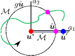
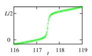
Figure 2: (top left) Schematic of the first Fourier mode slice, with $a_{1},\,a_{2}$ defined in the text. In this projection the slice border is a zero-measure ‘point’ at the origin. (bottom) For a generic ergodic trajectory the phase velocity $c=\dot{\ell}(t)$ appears to encounter singularities whenever it approaches the slice border, which, however, is never reached Budanur et al. (2015). Closer inspection reveals a rapid but continuous change in the shift (top right) by $\approx L/2$ in the $\ell(t)-\overline{c}t$ Galilean frame, moving (for our parameter values) at $\overline{c}=1.1092$. These apparent jumps are well resolved: each ‘+’ corresponds to 10 time integration steps.

As group orbits are circles crossing perpendicular to the $a_{1}$-axis in this projection, $\langle\mbox{\boldmath$t$}(\hat{\mbox{\boldmath$u$}})|\mbox{\boldmath$t$}^{\prime}\rangle$ in (2) can only be zero if the circle shrinks to a point at the origin. This requires that both inner products $\langle\mbox{\boldmath$u$}|\mbox{\boldmath$u$}^{\prime}\rangle$ and $\langle\mbox{\boldmath$u$}\,|\,g(L/4)\,\mbox{\boldmath$u$}^{\prime}\rangle$ are zero at the same time, which has vanishing probability. While we thus avoid the slice border, there is a rapid change in $\theta$ by $\approx\pi$ (in $\ell$ units by $\approx L/2$) whenever the trajectory $(a_{1},a_{2})(t)$ sweeps past the origin, see the inset to Fig. 2. Rapid phase shifts notwithstanding, this choice of template has made possible the discovery and analysis of the many relative periodic orbits discussed below.

	$\overline{D}$	$\overline{c}$	#	$D_{KY}$	$\mu^{(max)}$	$\omega$ or $\theta$
$\textrm{TW}_{N4L/1.38}$	1.380	1.238	3	6.97	0.1809	0
$\textrm{TW}_{2.03}$	2.039	1.091	7	15.21	0.1159	0
$\textrm{TW}_{1.97}$	1.968	1.104	9	20.01	0.1549	0.259
$\textrm{TW}_{2.04}$	2.041	1.095	8	20.04	0.1608	0
$\textrm{TW}_{N4U/3.28}$	3.279	1.051	30	73.67	0.9932	3.136
$\textrm{RPO}_{6.66}$	1.806	1.122	3	7.99	0.0535	1.690
$\textrm{RPO}_{27.30}$	1.815	1.127	4	8.98	0.0678	0.961
$\textrm{RPO}_{13.19}$	1.839	1.119	5	9.68	0.0581	2.038
$\textrm{RPO}_{20.43}$	1.809	1.130	5	11.03	0.0771	+1
$\textrm{RPO}_{4.95}$	2.015	1.090	3	11.54	0.1509	1.643
$\textrm{RPO}_{7.72}$	1.708	1.141	5	11.62	0.0983	+1
$\textrm{RPO}_{15.46}$	1.781	1.027	7	12.69	0.1162	+1
$\textrm{RPO}_{9.74}$	2.050	1.088	7	12.87	0.1873	-1
$\textrm{RPO}_{23.36}$	1.980	1.113	6	13.37	0.1011	1.251
$\textrm{RPO}_{7.42}$	1.838	1.111	6	13.89	0.1195	0.388
$\textrm{RPO}_{17.46}$	1.917	1.122	6	14.67	0.0841	0.196
$\textrm{RPO}_{14.05}$	1.902	1.109	7	14.75	0.1403	-1
ergodic	1.956	1.109

Table 1: A subset of traveling waves and relative periodic orbits of the lowest Kaplan-Yorke dimension Frederickson et al. (1983), out of respectively 10 and 29 extracted so far and plotted in Fig. 4. Traveling waves are labeled by their dissipation rate, and relative periodic orbits are labeled by their period $T$. Listed are mean dissipation ${\overline{D}}$, mean down-stream phase velocity $\overline{c}$, the number of unstable eigen-directions (two per each complex pair), Kaplan-Yorke dimension $D_{KY}$, the real part of the largest stability eigenvalue/Floquet exponent $\mu^{(max)}$, and either the corresponding imaginary part $\omega^{(max)}$ for traveling waves, or the phase $\theta$ of the complex Floquet multiplier for relative periodic orbits, or its sign, if real: -1 indicates inverse hyperbolic.

‘Minimal flow units’ Jiménez and Moin (1991), which capture much of the statistical properties of turbulence, have been invaluable in analyzing fundamental self-sustaining processes Hamilton et al. (1995). Here, the fixed-flux Reynolds number for all calculations is $Re=DU/\nu=2500$, where lengths are non-dimensionalized by diameter $D$ and velocities are normalized by the mean axial speed $U$. The minimal flow unit is in the $m=4$ rotational subspace, such that $(r,\theta,z)\in[0,\frac{1}{2}]\times[0,\frac{\pi}{2}]\times[0,\frac{\pi}{1.7}]$. The size of the domain is more usefully measured in terms of wall units, $\nu/u_{\tau}$, where $u_{\tau}^{2}=-\nu\left.(\partial_{r}u_{z})\right|_{\mathrm{wall}}$, which allows comparison with flow units used in other geometries. In these units, the domain is of size $\Omega^{+}\approx[100,160,370]$ in the wall-normal, spanwise and streamwise dimensions, respectively. Our flow unit compares favorably with the minimal flow units for channel flow Jiménez and Moin (1991) $\Omega^{+}\approx[\,>40,100,250-350]$ and Couette flow Hamilton et al. (1995) $\Omega^{+}\approx[68,128,190]$. Recurrent flows have been identified in ref. Gibson et al. (2008) for a box of size $\Omega^{+}\approx[68,86,190]$. Our domain is sufficiently large to reproduce $Re_{\tau}=(D/2)u_{\tau}/\nu=100\pm 1$ to within 10% of its value in the infinite domain. The mean wall friction for turbulent flow is approximately 100% greater than that for laminar flow at this flow rate.

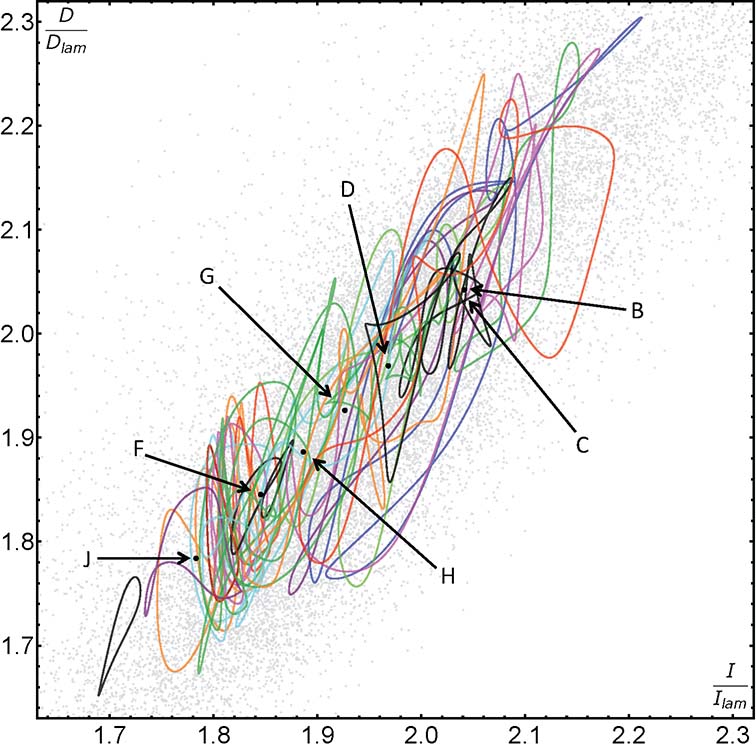
Figure 3: (Color online) Projection of 32 relative periodic orbits and traveling waves using symmetry-invariant coordinates, $I/I_{lam}$, $D/D_{lam}$ where $I_{lam}=D_{lam}$ are energy rates for the laminar flow. All discovered traveling waves are included: (B) $\textrm{TW}_{2.04}$, (C) $\textrm{TW}_{2.03}$, (D) $\textrm{TW}_{1.97}$, (G) $\textrm{TW}_{1.93}$, (H) $\textrm{TW}_{1.89}$, (F) $\textrm{TW}_{1.85}$ and (J) $\textrm{TW}_{1.78}$, except for $\textrm{TW}_{N4L/1.38}$, $\textrm{TW}_{N4U/3.28}$ and $\textrm{TW}_{1.57}$, which lie far outside the ergodic cloud (grey dots).

A Newton-Krylov scheme is used to search for relative periodic orbits. Initial guesses are taken from near recurrences of ergodic trajectories Gibson et al. (2008) within the symmetry-reduced state space. This preferentially identifies structures embedded in regions of high natural measure (regions most frequented by ergodic trajectories), with isolated traveling waves and relative periodic orbits that sit in the less frequented reaches of state space less likely to be found. Our searches have so far identified 10 traveling waves and 32 relative periodic orbits. An abbreviated summary of data is given in table 1; the complete data set is available online at Openpipeflow.org, along with the open source code used to calculate these orbits.

Visualizations of high-dimensional state space trajectories are necessarily projections onto two or three dimensions. A common choice is to monitor the flow in terms of the rate of energy dissipation $D=\rho\nu\int\mbox{\boldmath$u$}\cdot{\bf\nabla}^{2}\mbox{\boldmath$u$}\,dV$ and the external input power required to maintain constant flux $I=Q\,\Delta p$, where $Q=\int\mbox{\boldmath$u$}\cdot\mbox{\boldmath$dS$}$ is the flux at any cross-section and $\Delta p$ and is the pressure drop over the length of the pipe. As the time-averages of $I$ and $D$ are necessarily equal, traveling waves and orbits, which may be well-separated in state space, are contracted onto or near the $I=D$ line, a drawback of the 2-dimensional $(I,D)$ projection. Fig. 3 shows that the orbits appear to overlap with the ergodic region, but reveals little of the relationships between solutions; we use $D$ values only to distinguish traveling waves solutions listed in table 1.

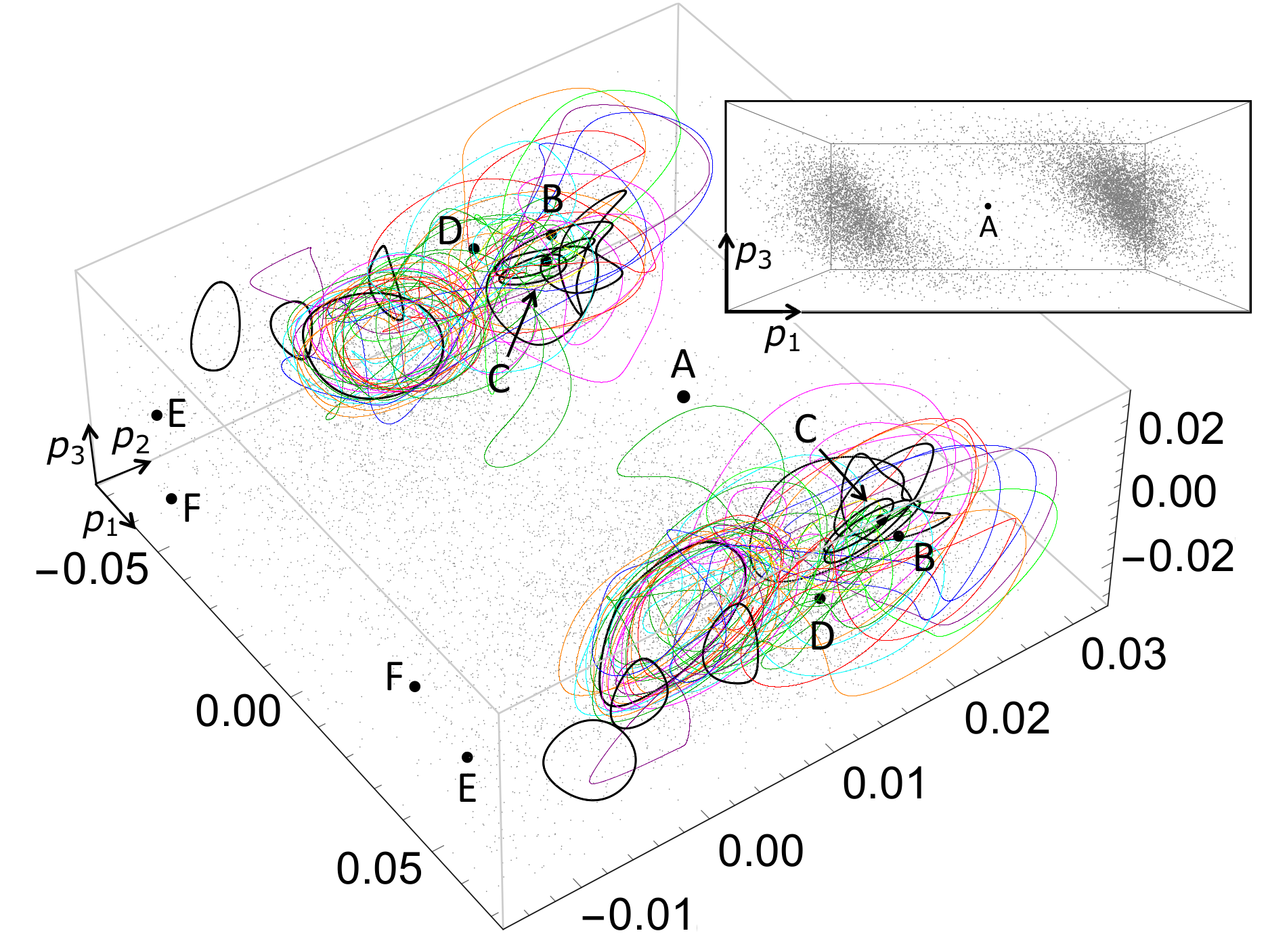
Figure 4: (Color online) Projection of the symmetry-reduced infinite-dimensional state space onto the first 3 PCA principal axes, computed from the L2-norm average over the natural measure (the gray ‘cloud’) in the slice. 32 relative periodic orbits, and a subset of the 7 shortest relative periodic orbits, together with traveling waves (A) $\textrm{TW}_{N4U/3.28}$, (B) $\textrm{TW}_{2.04}$, (C) $\textrm{TW}_{2.03}$, (D) $\textrm{TW}_{1.97}$, (E) $\textrm{TW}_{1.98}$, (F) $\textrm{TW}_{1.85}$. While $\textrm{TW}_{1.93}$ appears to lie in the very center of the $(I,D)$ projection Fig. 3, it is revealed in this state space projection to lie far from the ergodic cloud, outside the box plotted, as are (E) $\textrm{TW}_{N4L/1.38}$ and (F) $\textrm{TW}_{1.85}$. Due to a ‘rotate-and-reflect’ symmetry, each solution appears twice, with the exception of (A) $\textrm{TW}_{N4U/3.28}$ (and the far-away $\textrm{TW}_{N4L/1.38}$), which belong to the ‘rotate-and-reflect’ invariant subspace. Our relative periodic orbits capture the regions of high natural measure very well. The symmetry-invariant subspace has a strong repulsive influence, separating the natural measure into two weakly communicating regions. The inset shows the ergodic cloud from another perspective.

In the symmetry-reduced state space it is possible to construct coordinates that are intrinsic to the flow itself, using spatial information that would otherwise be smeared out by translational shifts. To obtain a global portrait of the turbulent set, Fig. 4, we project solutions onto the three largest principal components $\hat{\mbox{\boldmath$e$}}_{i}$ obtained from a PCA of $N$=2000 independent $\hat{\mbox{\boldmath$u$}}^{\prime}_{i}=\hat{\mbox{\boldmath$u$}}_{i}-\bar{\hat{\mbox{\boldmath$u$}}}$, where $\bar{\hat{\mbox{\boldmath$u$}}}$ is the mean of the data, using the SVD method (on average the square of the projection $p_{i}=\langle\hat{\mbox{\boldmath$u$}}^{\prime}(t)|\hat{\mbox{\boldmath$e$}}_{i}\rangle$ equals the $i^{\mathrm{th}}$ singular value of the correlation matrix $R_{ij}=\frac{1}{N-1}\langle\hat{\mbox{\boldmath$u$}}^{\prime}_{i}|\hat{\mbox{\boldmath$u$}}^{\prime}_{j}\rangle$).

The lower / upper branch pair $\textrm{TW}_{N4L/1.38}$ / $\textrm{TW}_{N4U/3.28}$ were obtained by continuation from a smaller ‘minimal flow unit’ Willis et al. (2013). In table 1 and in the $(I,D)$-projection Fig. 3 the upper branch traveling wave $\textrm{TW}_{N4U/3.28}$ appears to be far removed from turbulence, unlikely to exert influence. The PCA projection of the symmetry-reduced state space, however, reveals the strong repelling influence of $\textrm{TW}_{N4U/3.28}$ whose 30-dimensional unstable manifold acts as a barrier to the dynamics, cleaving the natural measure into two ‘clouds’, forcing a trajectory to hover around one neighborhood until it finds a path to the other, bypassing $\textrm{TW}_{N4U/3.28}$. The two ergodic ‘clouds’ are related by the ‘rotate-and-reflect’ symmetry ($\pi/4$ rotation), under which $\textrm{TW}_{N4U/3.28}$ is invariant (for symmetries of pipe flow see ref. Willis et al. (2013)).

The symmetry-reduced state space projections reveal sets of relative periodic orbits with qualitatively similar dynamics. The short-period orbits are well spread over the dense regions of natural measure, and the long relative periodic orbits in (a) appear to ‘shadow’ short orbits in (b), but also exhibit extended excursions that fill out state space. While sets of relative periodic orbits often share comparable dissipation rates and Floquet exponents (table 1 and Openpipeflow.org data sets), it is the state space projections that are essential to establishing genuine relationships.

In summary, we have shown that symmetry reduction can be applied to a dynamical system of very high dimensions, here turbulent pipe flow. An appropriately constructed template renders the method of slices substantially more effective for projecting the dynamics and for Newton searches for invariant solutions. The method is general and can be applied to any dynamical system with continuous translational or rotational symmetry. Projections of the symmetry-reduced space reveal fundamental properties of the dynamics not evident prior to symmetry reduction. In the application at hand, to a turbulent pipe flow, the method has enabled us to identify for the first time a large set of relative periodic orbits embedded in turbulence, and to demonstrate that the key invariant solutions strongly influence turbulent dynamics. To follow this demonstration of the power of symmetry reduction, work is now underway to determine the relationship between relative periodic orbits Willis et al. (2015). Analysis of their unstable manifolds are expected to reveal the intimate links between traveling waves and relative periodic orbits, allowing for explicit construction of the invariant skeleton that gives shape to the strange attractor explored by turbulence.