Abstract

The Majorana nature of massive neutrinos will be crucially probed in the next-generation experiments of the neutrinoless double-beta ($0\nu 2\beta$) decay. The effective mass term of this process, $\langle m\rangle_{ee}$, may be contaminated by new physics. So how to interpret a discovery or null result of the $0\nu 2\beta$ decay in the foreseeable future is highly nontrivial. In this paper we introduce a novel three-dimensional description of $|\langle m\rangle_{ee}|$, which allows us to see its sensitivity to the lightest neutrino mass and two Majorana phases in a transparent way. We take a look at to what extent the free parameters of $|\langle m\rangle_{ee}|$ can be well constrained provided a signal of the $0\nu 2\beta$ decay is observed someday. To fully explore lepton number violation, all the six effective Majorana mass terms $\langle m\rangle_{\alpha\beta}$ (for $\alpha,\beta=e,\mu,\tau$) are calculated and their lower bounds are illustrated with the two-dimensional contour figures. The effect of possible new physics on the $0\nu 2\beta$ decay is also discussed in a model-independent way. We find that the result of $|\langle m\rangle_{ee}|$ in the normal (or inverted) neutrino mass ordering case modified by the new physics effect may somewhat mimic that in the inverted (or normal) mass ordering case in the standard three-flavor scheme. Hence a proper interpretation of a discovery or null result of the $0\nu 2\beta$ decay may demand extra information from some other measurements.

1 Introduction

One of the burning questions in nuclear and particle physics is whether massive neutrinos are the Majorana fermions [1]. The latter must be associated with the phenomena of lepton number violation (LNV), such as the neutrinoless double-beta ($0\nu 2\beta$) decays of some even-even nuclei in the form of $(A,Z)\to(A,Z+2)+2e^{-}$ [2]. On the other hand, the Majorana zero modes may have profound consequences or applications in solid-state physics [3]. That is why it is fundamentally important to verify the existence of elementary Majorana fermions in Nature. The most suitable candidate of this kind is expected to be the massive neutrinos [4].

However, the tiny masses of three known neutrinos make it extremely difficult to identify their Majorana nature. The most promising experimental way is to search for the $0\nu 2\beta$ decays. Thanks to the Schechter-Valle theorem [5], a discovery of the $0\nu 2\beta$ decay mode will definitely pin down the Majorana nature of massive neutrinos no matter whether this LNV process is mediated by other new physics (NP) particles or not. The rate of such a decay mode can be expressed as

$$\Gamma^{0\nu}=G^{0\nu}(Q,Z)\left|M^{0\nu}\right|^{2}\left|\langle m\rangle_{ee}\right|^{2}\;,$$ (1)

where $G^{0\nu}$ is the phase-space factor, $M^{0\nu}$ denotes the relevant nuclear matrix element (NME), and $\langle m\rangle_{ee}$ stands for the effective Majorana neutrino mass term. In the standard three-flavor scheme,

$$\langle m\rangle_{ee}=m_{1}U^{2}_{e1}+m_{2}U^{2}_{e2}+m_{3}U^{2}_{e3}\;$$ (2)

with $m_{i}$ (for $i=1,2,3$) being the neutrino masses and $U_{ei}$ being the matrix elements of the Pontecorvo-Maki-Nakagawa-Sakata (PMNS) neutrino mixing matrix [6]. Given current neutrino oscillation data [7], the three neutrinos may have a normal mass ordering (NMO) $m_{1}<m_{2}<m_{3}$ or an inverted mass ordering (IMO) $m_{3}<m_{1}<m_{2}$. In the presence of NP, $\langle m\rangle_{ee}$ is likely to be contaminated by extra contributions which can be either constructive or destructive. While an observation of the $0\nu 2\beta$ decay must point to an appreciable value of $|\langle m\rangle_{ee}|$, a null experimental result does not necessarily mean that massive neutrinos are the Dirac fermions because $\langle m\rangle_{ee}\sim 0$ is not impossible even though the neutrinos themselves are the Majorana particles [8, 9].

Hence how to interpret a discovery or null result of the $0\nu 2\beta$ decay in the foreseeable future is highly nontrivial and deserves special attention [10, 11, 12]. In this work we focus on the sensitivity of $|\langle m\rangle_{ee}|$ to the unknown parameters in the neutrino sector, which include the absolute neutrino mass scale, the Majorana CP-violating phases, and even possible NP contributions. Beyond the popular Vissani graph [13] which gives a two-dimensional description of the dependence of $|\langle m\rangle_{ee}|$ on the smallest neutrino mass, we introduce a novel three-dimensional description of the sensitivity of $|\langle m\rangle_{ee}|$ to both the smallest neutrino mass and the Majorana phases in the standard three-flavor scheme. We single out the Majorana phase which may make $|\langle m\rangle_{ee}|$ sink into a decline in the NMO case, and show that a constructive NP contribution is possible to compensate that decline and enhance $|\langle m\rangle_{ee}|$ to the level which more or less mimics the case of the IMO. On the other hand, the destructive NP contribution is not impossible to suppress $|\langle m\rangle_{ee}|$ to the level which is indiscoverable, even though the neutrino mass ordering is inverted or nearly degenerate. Given a discovery of the $0\nu 2\beta$ decay, the possibility of constraining the unknown parameters is discussed in several cases. We also examine the dependence of $|\langle m\rangle_{\alpha\beta}|$ (for $\alpha,\beta=e,\mu,\tau$) on the absolute neutrino mass scale and three CP-violating phases of the PMNS matrix $U$, and conclude that some other possible LNV processes have to be measured in order to fully understand an experimental outcome of the $0\nu 2\beta$ decay and even determine the Majorana phases.

2 A three-dimensional description of $|\langle m\rangle_{ee}|$

In the standard three-flavor scheme the unitary PMNS matrix $U$ can be parameterized in terms of three rotation angles ($\theta_{12}$, $\theta_{13}$, $\theta_{23}$) and three phase angles ($\delta$, $\rho$, $\sigma$) in the following way [7]:

$$U_{e1}=c_{12}c_{13}\ e^{{\rm i}\rho/2}\;,\hskip 35.56593ptU_{e2}=s_{12}c_{13}\;,$$

$$U_{e3}=s_{13}\ e^{{\rm i}\sigma/2}\;,\hskip 48.36958ptU_{\mu 3}=c_{13}s_{23}\ e^{{\rm i}\left(\delta+\rho/2\right)}\;,\hskip 14.22636pt$$ (3)

where $c_{ij}\equiv\cos\theta_{ij}$ and $s_{ij}\equiv\sin\theta_{ij}$ (for $ij=12,13,23$), $\delta$ is referred to as the Dirac phase since it measures the strength of CP violation in neutrino oscillations, $\rho$ and $\sigma$ are referred to as the Majorana phases and have nothing to do with neutrino oscillations. The phase convention taken in Eq. (3) is intended to forbid $\delta$ to appear in the effective Majorana mass term of the $0\nu 2\beta$ decay:

$$\left|\langle m\rangle_{ee}\right|=\left|m_{1}c_{12}^{2}c_{13}^{2}\ e^{{\rm i}\rho}+m_{2}s_{12}^{2}c_{13}^{2}+m_{3}s_{13}^{2}\ e^{{\rm i}\sigma}\right|\;.$$ (4)

The merit of this phase convention is obvious. In the extreme case of the NMO or IMO (i.e., $m_{1}=0$ or $m_{3}=0$), which is allowed by current experimental data, one of the two Majorana phases automatically disappears from $|\langle m\rangle_{ee}|$. Note, however, that $\delta$ is intrinsically of the Majorana nature because it can enter other effective Majorana mass terms (e.g., $\langle m\rangle_{e\mu}$ and $\langle m\rangle_{\mu\tau}$ [14]).

A measurement of the $0\nu 2\beta$ decay allows us to determine or constrain $|\langle m\rangle_{ee}|$. So far the most popular way of presenting $|\langle m\rangle_{ee}|$ has been the Vissani graph [13]. It illustrates the allowed range of $|\langle m\rangle_{ee}|$ against $m_{1}$ or $m_{3}$ by inputting the experimental values of $\theta_{12}$ and $\theta_{13}$ and allowing $\rho$ and $\sigma$ to vary in the interval $[0^{\circ},360^{\circ})$. In the NMO case $|\langle m\rangle_{ee}|$ may sink into a decline when $m_{1}$ lies in the range $0.0023$ eV — $0.0063$ eV [15], implying a significant or complete cancellation among the three components of $|\langle m\rangle_{ee}|$. In comparison, there is a lower bound $|\langle m\rangle_{ee}|\gtrsim 0.02$ eV in the IMO case, and it is always larger than the upper bound of $|\langle m\rangle_{ee}|$ in the NMO case when the lightest neutrino mass is smaller than about 0.01 eV [15]. This salient feature enables us to confirm or rule out the IMO, if the future $0\nu 2\beta$-decay experiments can reach a sensitivity below 0.02 eV. Nevertheless, the Vissani graph is unable to tell the dependence of $|\langle m\rangle_{ee}|$ on $\rho$ and $\sigma$. For example, which Majorana phase is dominantly responsible for the significant decline of $|\langle m\rangle_{ee}|$ in the NMO case? To answer such questions and explore the whole parameter space, let us generalize the two-dimensional Vissani graph by introducing a novel three-dimensional description of $|\langle m\rangle_{ee}|$.

Fig. 1 is a three-dimensional illustration of the lower and upper bounds of $|\langle m\rangle_{ee}|$ in the NMO and IMO cases. In our numerical calculations we have input the best-fit values of $\Delta m^{2}_{21}$, $\Delta m^{2}_{31}$, $\theta_{12}$ and $\theta_{13}$ obtained from a recent global analysis of current neutrino oscillation data [16]. For simplicity, the uncertainties of these four parameters are not taken into account because they do not change the main features of $|\langle m\rangle_{ee}|$. The unknown Majorana phases $\rho$ and $\sigma$ are allowed to vary in the range $[0^{\circ},360^{\circ})$, and the neutrino mass $m_{1}$ or $m_{3}$ is constrained via the Planck data (i.e., $m_{1}+m_{2}+m_{3}<0.23$ eV at the $95\%$ confidence level [17]). Some comments on Fig. 1 are in order. (1) The upper bound of $|\langle m\rangle_{ee}|$ is trivial, because it can be obtained by simply taking $\rho=\sigma=0^{\circ}$. (2) The lower bound of $|\langle m\rangle_{ee}|$ is nontrivial, because it is a result of the maximal cancellation among the three components of $|\langle m\rangle_{ee}|$ for given values of $\rho$, $\sigma$ and $m_{1}$ or $m_{3}$. (3) In the NMO case it is the phase $\rho$ that may lead the lower bound of $|\langle m\rangle_{ee}|$ to a significant decline (even down to zero). In comparison, $|\langle m\rangle_{ee}|$ is essentially insensitive to $\sigma$ in both the NMO and IMO cases. (4) The allowed range of $|\langle m\rangle_{ee}|$ in the IMO case exhibits a “steady flow” profile, which is consistent with the two-dimensional Vissani graph. Its lower bound ($\sim 0.02$ eV) appears at $\rho=180^{\circ}$ for a specific value of $m_{3}$ and arbitrary values of $\sigma$, but a deadly cancellation among the three components of $|\langle m\rangle_{ee}|$ has no way to happen. (5) When the neutrino mass spectrum is nearly degenerate (i.e., $m_{1}\simeq m_{2}\simeq m_{3}\gtrsim 0.05$ eV), the results of $|\langle m\rangle_{ee}|$ in the NMO and IMO cases are almost indistinguishable.

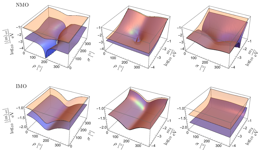
Figure 1: Three-dimensional illustration of the lower (blue) and upper (light orange) bounds of $|\langle m\rangle_{ee}|$ as functions of the lightest neutrino mass and two Majorana phases in the NMO or IMO case.

The parameter space for the vanishing of $|\langle m\rangle_{ee}|$ in the NMO case is of particular interest, because it points to a null result of the $0\nu 2\beta$ decay although massive neutrinos are the Majorana particles. However, the “dark well” of $|\langle m\rangle_{ee}|$ versus the $\rho$-$m_{1}$ plane in Fig. 1 has a sharp champagne-bottle profile at the ground. This characteristic can be understood by figuring out the correlation between $m_{1}$ and $\rho$ from $|\langle m\rangle_{ee}|=0$. Namely,

$$m_{1}^{2}c_{12}^{4}c_{13}^{4}+2m_{1}m_{2}c_{12}^{2}s_{12}^{2}c^{4}_{13}\cos\rho+m_{2}^{2}s^{4}_{12}c_{13}^{4}=m_{3}^{2}s_{13}^{4}\ .$$ (5)

Given the best-fit values of $\Delta m^{2}_{21}$, $\Delta m^{2}_{31}$, $\theta_{12}$ and $\theta_{13}$ [16], Fig. 2 shows the $\rho$-$m_{1}$ correlation which corresponds to the contour of the champagne-bottle profile of $|\langle m\rangle_{ee}|$ in Fig. 1. One can see that the “dark well” appears when $\rho$ lies in the range $160^{\circ}$ — $200^{\circ}$ and $m_{1}$ varies from $0.0023$ eV to $0.0063$ eV for arbitrary values of $\sigma$. Such a fine structure of cancellation has been missed before.

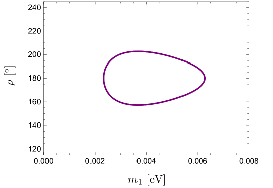
Figure 2: A correlation between $m_{1}$ and $\rho$ as constrained by the vanishing of $|\langle m\rangle_{ee}|$ in the NMO case, corresponding to the contour of the champagne-bottle profile of $|\langle m\rangle_{ee}|$ in Fig. 1.

As a matter of fact, a three-dimensional description of $|\langle m\rangle_{ee}|$ against two free parameters is equivalent to a set of two-dimensional contour figures which project the values of $|\langle m\rangle_{ee}|$ onto the parameter-space planes, if only its upper or lower bound is considered. In order to clearly present the correspondence between the numerical result of $|\langle m\rangle_{ee}|$ and that of a given parameter which is difficult to be identified in a three-dimensional graph, we show the contour figures for the lower bound of $|\langle m\rangle_{ee}|$ on the $\rho$-$\sigma$, $m_{1}$-$\rho$ (or $m_{3}$-$\rho$) and $m_{1}$-$\sigma$ (or $m_{3}$-$\sigma$) planes in the NMO (or IMO) case in Fig. 3 (or Fig. 4). For the sake of completeness, we calculate the contour figures for the lower bounds of all the six effective Majorana mass terms defined as

$$\langle m\rangle_{\alpha\beta}=m_{1}U_{\alpha 1}U_{\beta 1}+m_{2}U_{\alpha 2}U_{\beta 2}+m_{3}U_{\alpha 3}U_{\beta 3}\;,$$ (6)

where the subscripts $\alpha$ and $\beta$ run over $e$, $\mu$ and $\tau$. There are at least two good reasons for considering $|\langle m\rangle_{\alpha\beta}|$: (a) only the $0\nu 2\beta$ decay itself cannot offer sufficient information to fix the three unknown parameters of $|\langle m\rangle_{ee}|$; (b) if a null result of the $0\nu 2\beta$ decay is observed, one will have to search for some other LNV processes so as to identify the Majorana nature of massive neutrinos. The typical LNV processes which are associated with $\langle m\rangle_{\alpha\beta}$ include the $\mu^{-}\to e^{+}$ conversion in the nuclear background, neutrino-antineutrino oscillations, rare LNV decays of $B$ and $D$ mesons, and so on [15]. In Figs. 3 and 4 the contours for the lower bounds of $|\langle m\rangle_{\alpha\beta}|$ are presented by gradient colors and their corresponding magnitudes are indicated by the legends. In particular, the purple areas stand for the parameter space where significant cancellations (i.e., $|\langle m\rangle_{\alpha\beta}|<10^{-4}$ eV) can take place. When the $m_{3}$-associated term of $|\langle m\rangle_{\alpha\beta}|$ is not suppressed by $s^{2}_{13}\sim 2\%$, its lower bound becomes sensitive to the Majorana phase $\sigma$. Hence a combined analysis of the $0\nu 2\beta$ decay and some other LNV processes will be greatly helpful to determine or constrain both $\rho$ and $\sigma$.

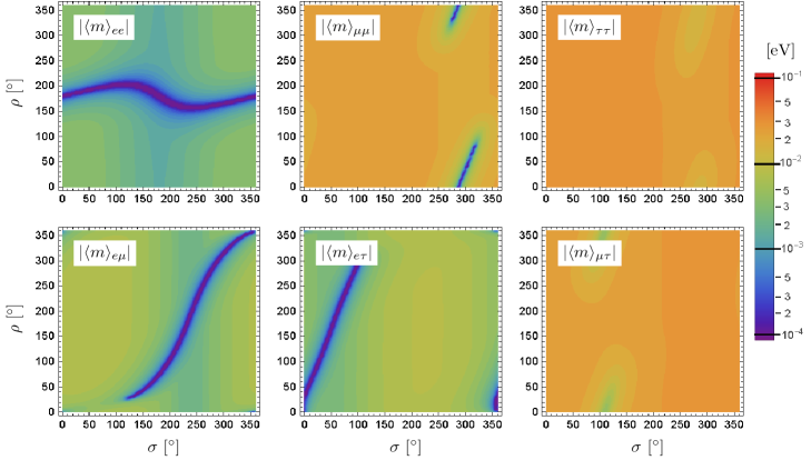
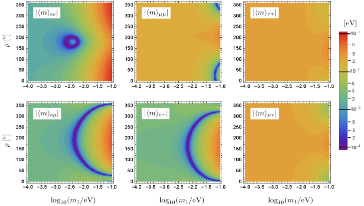
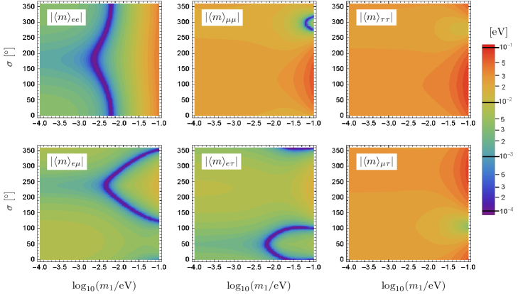
Figure 3: The lower bounds of $|\langle m\rangle_{\alpha\beta}|$ changing with $m_{1}$, $\rho$ and $\sigma$ in the NMO case.

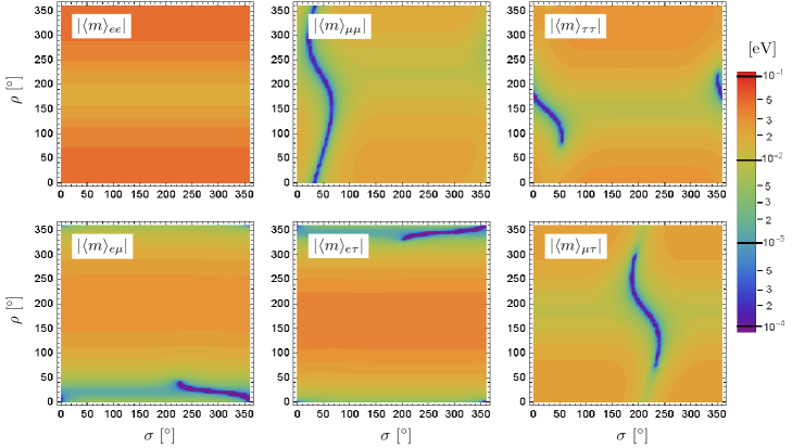
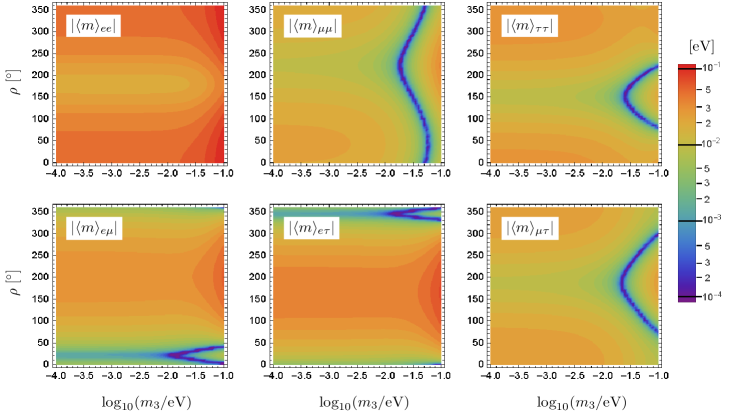
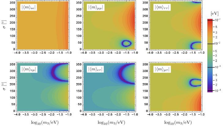
Figure 4: The lower bounds of $|\langle m\rangle_{\alpha\beta}|$ changing with $m_{3}$, $\rho$ and $\sigma$ in the IMO case.

3 Limits of $m_{1,3}$ and $\rho$ from a signal of the $0\nu 2\beta$ decay

In the standard three-flavor scheme we have studied the possible profile (especially the lower bound) of $|\langle m\rangle_{ee}|$ against the unknown mass and phase parameters. Inversely, the unknown parameters can be constrained if the $0\nu 2\beta$ decay is discovered and the magnitude of $|\langle m\rangle_{ee}|$ is determined. A good example of this kind is the strong constraint on the parameter space of $m_{1}$ and $\rho$ in Eq. (5) or Fig. 2 based on the assumption $|\langle m\rangle_{ee}|=0$, which is more or less equivalent to a null result of the $0\nu 2\beta$ decay provided the experimental sensitivity has been good enough. So it makes sense to ask the following question: to what extent the unknown parameters can be constrained from a signal of the $0\nu 2\beta$ decay?

Let us try to answer this question in an ideal situation with no concern about the experimental error bars. The first issue is to derive the correlation between $m_{1}$ (or $m_{3}$) and $\rho$ like that given in Eq. (5) by eliminating $\sigma$. Since Eq. (4) can be viewed as an implicit function $\rho=f(m_{i},\sigma)$ for given values of $\theta_{12}$, $\theta_{13}$ and $|\langle m\rangle_{ee}|$, one may eliminate $\sigma$ by substituting it with the solution of $\partial\rho/\partial\sigma|_{\sigma^{*}}=0$. In this way we obtain the maximum and minimum of $\rho$ as functions of $m_{i}$:

$$\cos\rho_{\text{max,min}}=-\frac{m_{1}^{2}c_{12}^{4}c_{13}^{4}+m_{2}^{2}s^{4}_{12}c_{13}^{4}-\left(m_{3}s_{13}^{2}\pm|\langle m\rangle_{ee}|\right)^{2}}{2m_{1}m_{2}c_{12}^{2}s_{12}^{2}c^{4}_{13}}\;.$$ (7)

If $|\langle m\rangle_{ee}|$ vanishes, then it is straightforward for Eq. (7) to reproduce Eq. (5). The maximum and minimum of $\sigma$ as functions of $m_{i}$ can similarly be obtained:

$$\cos\sigma_{\text{max,min}}=-\frac{m_{3}^{2}s_{13}^{4}+m_{2}^{2}s^{4}_{12}c_{13}^{4}-\left(m_{1}c_{12}^{2}c_{13}^{2}\pm|\langle m\rangle_{ee}|\right)^{2}}{2m_{2}m_{3}s_{12}^{2}c_{13}^{2}s^{2}_{13}}\;.$$ (8)

However, $\sigma$ is actually insensitive to $|\langle m\rangle_{ee}|$ as shown in Fig. 1. Hence the constraint on $\sigma$ must be rather loose even if the $0\nu 2\beta$ decay is observed. For this reason we simply focus on the possible constraints on $\rho$ and $m_{1}$ (or $m_{3}$) in the following.

Of course, the value of $|\langle m\rangle_{ee}|$ extracted from a measurement of the $0\nu 2\beta$ decay via Eq. (1) must involve a large uncertainty originating from the NME $M^{0\nu}$, while the phase-space factor $G^{0\nu}(Q,Z)$ can be precisely calculated. Following Ref. [18], we introduce a dimensionless factor $F$ to parameterize the uncertainty of $|\langle m\rangle_{ee}|$ inheriting from that of the NME: $F=M^{0\nu}_{\text{max}}/M^{0\nu}_{\text{min}}$, where $M^{0\nu}_{\text{max}}$ and $M^{0\nu}_{\text{min}}$ stand respectively for the maximal and minimal values of the NME which are consistently calculated in a given framework. It is apparent that $F\gtrsim 1$ holds, and $F=1$ cannot be reached until the NME is accurately determined. Given a value of $F$, the “true” value of $|\langle m\rangle_{ee}|$ may lie in the range $\big{[}|\langle m\rangle_{ee}|/\sqrt{F},\ |\langle m\rangle_{ee}|\sqrt{F}\big{]}$ [18]. In our numerical calculation we take $F=1$ and $F=2$ for illustration. Fig. 5 shows the allowed regions of $m_{1}$ (or $m_{3}$) and $\rho$ for a few typical values of $|\langle m\rangle_{ee}|$. The effect of $F$ can be seen when comparing between the cases of $F=1$ and $F=2$. Two comments are in order. (1) If $|\langle m\rangle_{ee}|$ is vanishingly small (e.g., $|\langle m\rangle_{ee}|=0.0005$ eV), $\rho$ can be constrained in the range $[140^{\circ},220^{\circ}]$ in the NMO case. If a larger value of $|\langle m\rangle_{ee}|$ is measured (e.g., $0.005$ eV or $0.05$ eV), the allowed range of $\rho$ will saturate the full interval $[0,360^{\circ})$. To fix the value of $\rho$ needs the input of $m_{1}$. Hence some additional information about $m_{1}$ from the cosmological observation or from the direct beta-decay experiment will be greatly helpful. (2) The situation in the IMO case is quite similar: $\rho$ can be constrained in a narrow range if $|\langle m\rangle_{ee}|$ approaches its minimal value (i.e., $0.02$ eV), but it is allowed to take any value in the range $[0,360^{\circ})$ if $|\langle m\rangle_{ee}|$ is much larger (e.g., $0.05$ eV). Here again is some additional information about $m_{3}$ required to pin down the value of $\rho$.

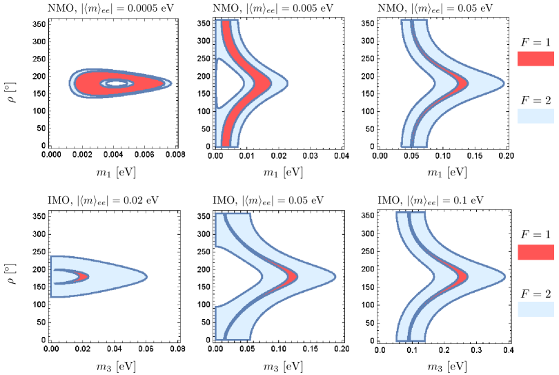
Figure 5: The regions of the smallest neutrino mass ($m_{1}$ or $m_{3}$) and the Majorana phase $\rho$ as constrained by an “observed” value of $|\langle m\rangle_{ee}|$. In the NMO case $|\langle m\rangle_{ee}|=0.0005$ eV, $0.005$ eV and $0.05$ eV are taken, and in the IMO case $|\langle m\rangle_{ee}|=0.02$ eV, $0.05$ eV and $0.1$ eV are input. The NME uncertainty is illustrated by $F$.

4 Possible NP contributions to $|\langle m\rangle_{ee}|$

When a NP contribution to the $0\nu 2\beta$ decay is concerned, the situation can be quite complicated because it may compete with the standard effect (i.e., the one from the three light Majorana neutrinos as discussed above) either constructively or destructively. If the NP effect is significant enough, the simple relation between $\Gamma^{0\nu}$ and $|\langle m\rangle_{ee}|$ in Eq. (1) has to be modified. This will make the interpretation of a discovery or null result of the $0\nu 2\beta$ decay more uncertain. Here we aim to study the issue in a model-independent way. Namely, we parameterize the possible NP contribution to $|\langle m\rangle_{ee}|$ in terms of its modulus and phase relative to the standard contribution, without going into details of any specific NP model [19, 20].

An interesting and very likely case is that different contributions can add in a coherent way so that their constructive or destructive interference may happen [19, 21]. If the helicities of two electrons emitted in the NP-induced $0\nu 2\beta$ channel are identical to those in the standard channel, then the overall rate of the $0\nu 2\beta$ decay in Eq. (1) can be modified in the following way:

$$\Gamma^{0\nu} = G^{0\nu}(Q,Z)\left|M^{0\nu}\langle m\rangle_{ee}+M_{\rm NP}^{0\nu}m_{\rm NP}^{0}\right|^{2}$$ (9)

$$\equiv G^{0\nu}(Q,Z)\left|M^{0\nu}\right|^{2}\left|\langle m\rangle_{ee}^{\prime}\right|^{2}\;,$$

where $M_{\rm NP}^{0\nu}$ denotes the NME subject to the NP process, $m_{\rm NP}^{0}$ is a particle-physics parameter describing the NP contribution, and $\langle m\rangle_{ee}^{\prime}$ represents the effective Majorana mass term defined as

$$\langle m\rangle_{ee}^{\prime}=m_{1}U^{2}_{e1}+m_{2}U^{2}_{e2}+m_{3}U^{2}_{e3}+m_{\rm NP}\;$$ (10)

with $m_{\rm NP}\equiv m_{\rm NP}^{0}M_{\rm NP}^{0\nu}/M^{0\nu}$. Unless $M_{\rm NP}^{0\nu}$ is identical with $M^{0\nu}$ like the case of NP coming from the light sterile neutrinos [22], $m_{\rm NP}$ generally differs from one isotope to another. Hence using different isotopes to detect the $0\nu 2\beta$ decays is helpful for us to learn whether there is NP beyond the standard scenario, but their different NMEs may involve different uncertainties.

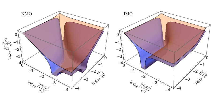
Figure 6: The lower (blue) and upper (light orange) bounds of $|\langle m\rangle_{ee}^{\prime}|$ as functions of $m_{1}$ (or $m_{3}$) and $|m_{\rm NP}|$ in the NMO (or IMO) case.

To see the interference between the NP term $m_{\rm NP}=|m_{\rm NP}|e^{{\rm i}\phi_{\rm NP}}$ and the standard one $\langle m\rangle_{ee}$ in $|\langle m\rangle^{\prime}_{ee}|$, we plot the lower and upper bounds of $|\langle m\rangle^{\prime}_{ee}|$ vs $m_{1}$ (or $m_{3}$) and $|m_{\rm NP}|$ in the NMO (or IMO) case in Fig. 6. For given values of $m_{1}$ (or $m_{3}$) and $|m_{\rm NP}|$, the lower and upper bounds of $|\langle m\rangle^{\prime}_{ee}|$ can be expressed as

$$\left|\langle m\rangle^{\prime}_{ee}\right|_{\rm upper} = m_{1}\left|U_{e1}\right|^{2}+m_{2}\left|U_{e2}\right|^{2}+m_{3}\left|U_{e3}\right|^{2}+|m_{\rm NP}|\;,$$

$$\left|\langle m\rangle^{\prime}_{ee}\right|_{\rm lower} = \max\Big{\{}0,~{}2m_{i}\left|U_{ei}\right|^{2}-\left|\langle m\rangle^{\prime}_{ee}\right|_{\rm upper},~{}2\left|m_{\rm NP}\right|-\left|\langle m\rangle^{\prime}_{ee}\right|_{\rm upper}\Big{\}}\;$$ (11)

for $i=1,2,3$. These results can be directly derived with the help of the “coupling-rod” diagram of the $0\nu 2\beta$ decay in the presence of the NP [9]. By setting $m_{\text{NP}}\to 0$, we simply arrive at the results of $|\langle m\rangle_{ee}|$ obtained before in the standard three-flavor scheme [13]. Some comments on our numerical results are in order.

(1) The parameter space in the NMO case can be divided into three regions according to the profile of the lower bound of $|\langle m\rangle^{\prime}_{ee}|$: (a) the region with $m_{1}<0.001$ eV and $|m_{\rm NP}|<0.001$ eV, where the NP contribution is negligibly small and thus $|\langle m\rangle^{\prime}_{ee}|$ approximates to

$$\left|\langle m\rangle_{ee}^{\prime}\right|\simeq\left|\langle m\rangle_{ee}\right|\gtrsim\left|\sqrt{\Delta m_{21}^{2}}\ s^{2}_{12}c_{13}^{2}-\sqrt{\Delta m_{31}^{2}}\ s_{13}^{2}\right|\;;$$ (12)

(b) the region with $m_{1}>0.01$ eV and $|\langle m\rangle_{ee}|$ being still dominant over $|m_{\rm NP}|$, where $|\langle m\rangle_{ee}^{\prime}|$ has a lower bound

$$\left|\langle m\rangle_{ee}^{\prime}\right|\simeq\left|\langle m\rangle_{ee}\right|\gtrsim\left|m_{1}c_{12}^{2}c_{13}^{2}-\sqrt{m_{1}^{2}+\Delta m_{21}^{2}}\ s_{12}^{2}c_{13}^{2}-\sqrt{m_{1}^{2}+\Delta m_{31}^{2}}\ s_{13}^{2}\right|\;;$$ (13)

and (c) the region with $|m_{\rm NP}|$ being dominant over $|\langle m\rangle_{ee}|$, where the lower bound of $|\langle m\rangle_{ee}^{\prime}|$ is simply the value of $|m_{\rm NP}|$. If $|m_{\rm NP}|$ is comparable in magnitude with $|\langle m\rangle_{ee}|$ of the IMO case in the standard three-flavor scheme, it will be impossible to distinguish the NMO case with NP from the IMO case without NP by only measuring the $0\nu 2\beta$ decay. This observation would make sense in the following situation: a signal of the $0\nu 2\beta$ decay looking like the IMO case in the standard scenario were measured someday, but the IMO itself were in conflict with the “available” cosmological constraint on the sum of three neutrino masses. Note also that at the junctions of the aforementioned three regions, $|\langle m\rangle_{ee}^{\prime}|$ can be vanishingly small either because $|\langle m\rangle_{ee}|$ and $|m_{\rm NP}|$ are both very small or because they undergo a deadly cancellation.

(2) The profile of the lower bound of $|\langle m\rangle_{ee}^{\prime}|$ in the IMO case is structurally simpler, as shown in Fig. 6. In the region dominated by $|\langle m\rangle_{ee}|$, $|\langle m\rangle_{ee}^{\prime}|$ just behaves like $|\langle m\rangle_{ee}|$ in the standard scenario and has a lower bound:

$$\left|\langle m\rangle_{ee}^{\prime}\right|\simeq\left|\langle m\rangle_{ee}\right|\gtrsim\left|m_{1}c_{12}^{2}c_{13}^{2}-\sqrt{m_{1}^{2}+\Delta m_{21}^{2}}\ s_{12}^{2}c_{13}^{2}\right|\;.$$ (14)

On the other hand, $|\langle m\rangle_{ee}^{\prime}|$ will be saturated by $|m_{\rm NP}|$ when the latter is dominant over $|\langle m\rangle_{ee}|$. At the junction of these two regions, $\langle m\rangle_{ee}$ and $m_{\rm NP}$ are comparable in magnitude and have a chance to cancel each other. This unfortunate possibility would deserve special attention if the IMO were verified by the cosmological data but a signal of the $0\nu 2\beta$ decay were not observed in an experiment sensitive to the $|\langle m\rangle_{ee}|$ interval in the IMO case of the standard scenario.

5 Summary

While most of the particle theorists believe that massive neutrinos must be the Majorana fermions, an experimental test of this belief is mandatory. Today a number of $0\nu 2\beta$-decay experiments are underway for this purpose. It is therefore imperative to consider how to interpret a discovery or null result of the $0\nu 2\beta$ decay beforehand, before this will finally turn into reality.

In this work we have tried to do so by presenting some new ideas and results which are essentially different from those obtained before. First, we have introduced a three-dimensional description of the effective Majorana mass term $|\langle m\rangle_{ee}|$ by going beyond the conventional Vissani graph. This new description allows us to look into the sensitivity of $|\langle m\rangle_{ee}|$ (especially its lower bound) to the lightest neutrino mass and two Majorana phases in a more transparent way. For example, we have shown that it is the Majorana phase $\rho\sim\pi$ that may make $|\langle m\rangle_{ee}|$ sink into a decline in the NMO case. Second, we have extended our discussion to all the six effective Majorana masses $|\langle m\rangle_{\alpha\beta}|$ (for $\alpha,\beta=e,\mu,\tau$) which are associated with a number of different LNV processes, and presented a set of two-dimensional contour figures for their lower bounds. We stress that such a study makes sense because a measurement of the $0\nu 2\beta$ decay itself does not allow us to pin down the two Majorana phases. Third, we have studied to what extent $m_{1}$ (or $m_{3}$) and $\rho$ can be well constrained provided a discovery of the $0\nu 2\beta$ decay (i.e., a definite value of $|\langle m\rangle_{ee}|$) is made someday. It is found that the smaller $|\langle m\rangle_{ee}|$ is, the stronger the constraint will be. Finally, the effect of possible NP contributing to the $0\nu 2\beta$ decay has been discussed in a model-independent way. It is of particular interest to find that the NMO (or IMO) case modified by the NP effect may more or less mimic the IMO (or NMO) case in the standard three-flavor scheme. In this case a proper interpretation of a discovery or null result of the $0\nu 2\beta$ decay demands an input of extra information about the absolute neutrino mass scale and (or) Majorana phases from some other measurements.

In any case it is fundamentally important to identify the Majorana nature of massive neutrinos. While there is still a long way to go in this connection, we hope that our study may help pave the way for reaching the exciting destination.

We would like to thank A. Palazzo for calling our attention to an error in the previous version of this paper. This work was supported in part by the National Natural Science Foundation of China under grant No. 11375207 and No. 11135009.

References

- [1] E. Majorana, Nuovo Cim. 14, 171 (1937).
- [2] W.H. Furry, Phys. Rev. 56, 1184 (1939).
- [3] S.R. Elliot and M. Franz, Rev. Mod. Phys. 87, 137 (2015).
- [4] B. Pontecorvo, Sov. Phys. JETP 6, 429 (1957).
- [5] J. Schechter and J.W.F. Valle, Phys. Rev. D 25, 2951 (1982).
- [6] Z. Maki, M. Nakagawa, and S. Sakata, Prog. Theor. Phys. 28, 870 (1962); B. Pontecorvo, Sov. Phys. JETP 26, 984 (1968).
- [7] K.A. Olive et al. (Particle Data Group), Chin. Phys. C 38, 090001 (2014).
- [8] Z.Z. Xing, Phys. Rev. D 68, 053002 (2003).
- [9] Z.Z. Xing and Y.L. Zhou, Chin. Phys. C 39, 011001 (2015).
- [10] For instance, some particular attention has been paid to the role of the Majorana phases in the decay in: S.M. Bilenky, S. Pascoli and S.T. Petcov, Phys. Rev. D 64, 053010 (2001); S. Pascoli, S.T. Petcov and L. Wolfenstein, Phys. Lett. B 524, 319 (2002); V. Barger, S.L. Glashow, P. Langacker and D. Marfatia, Phys. Lett. B 540, 247 (2002); H. Nunokawa, W.J.C. Teves and R. Zukanovich Funchal, Phys. Rev. D 66, 093010 (2002); S. Pascoli, S.T. Petcov and W. Rodejohann, Phys. Lett. B 549, 177 (2002); F. Deppisch, H. Ps and J. Suhonen, Phys. Rev. D 72, 033012 (2005); F. Simkovic, S.M. Bilenky, A. Faessler and T. Gutsche, Phys. Rev. D 87, 073002 (2013); A. Faessler, G.L. Fogli, E. Lisi, V. Rodin, A.M. Rotunno, F. Simkovic, Phys. Rev. D 87, 053002 (2013).
- [11] S.M. Bilenky, C. Giunti, C.W. Kim and S.T. Petcov, Phys. Rev. D 54, 4432 (1996); H. Minakata and O. Yasuda, Phys. Rev. D 56, 1692 (1997); V.D. Barger and K.Whisnant, Phys. Lett. B 456, 194 (1999); M. Czakon, J. Gluza and M. Zralek, Phys. Lett. B 465, 211 (1999); M. Czakon, J. Gluza, J. Studnik and M. Zralek, Phys. Rev. D 65, 053008 (2002); Z.Z. Xing, Phys. Rev. D 65, 077302 (2002); S. Choubey and W. Rodejohann, Phys. Rev. D 72, 033016 (2005).
- [12] S. Dell’Oro, S. Marcocci, and F. Vissani, Phys. Rev. D 90, 033005 (2014).
- [13] F. Vissani, JHEP 06, 022 (1999).
- [14] Z.Z. Xing, Phys. Rev. D 87, 053019 (2013); Z.Z. Xing and Y.L. Zhou, Phys. Rev. D 88, 033002 (2013).
- [15] For the latest review with extensive references, see: S.M. Bilenky and C. Giunti, Int. J. Mod. Phys. A 30, 0001 (2015).
- [16] M. C. Gonzalez-Garcia, M. Maltoni and T. Schwetz, JHEP 1411, 052 (2014).
- [17] P.A.R. Ade et al. (Planck Collaboration), arXiv:1502.01589 [astro-ph.CO].
- [18] S. Pascoli, S. T. Petcov and T. Schwetz, Nucl. Phys. B 734, 24 (2006); H. Minakata, H. Nunokawa and A. A. Quiroga, PTEP 2015, 033B03 (2015).
- [19] For a review with extensive references, see: W. Rodejohann, Int. J. Mod. Phys. E 20, 1833 (2011); H.V. Klapdor-Kleingrothaus, hep-ex/9901021 (1999).
- [20] For some recent discussions, see: J. Lopez-Pavon, S. Pascoli and C.F. Wong, Phys. Rev. D 87, 093007 (2013); A. Meroni, S.T. Petcov and F. Simkovic, JHEP 1302, 025 (2013); S. Pascoli, M. Mitra and S. Wong, Phys. Rev. D 90, 093005 (2014).
- [21] See, e.g., G. Belanger, F. Boudjema, D. London, and H. Nadeau, Phys. Rev. D 53, 6292 (1996); Z.Z. Xing, Phys. Lett. B 679, 255 (2009).
- [22] See, e.g., Z.Z. Xing, Phys. Rev. D 85, 013008 (2012); Y.F. Li and S.S. Liu, Phys. Lett. B 706, 406 (2012).