Standard Electroweak Interactions
in Gravitational Theory with Chameleon Field and Torsion

Abstract

We propose a version of a gravitational theory with the torsion field, induced by the chameleon field. Following Hojman et al. Phys. Rev. D 17, 3141 (1976) the results, obtained in Phys. Rev. D 90, 045040 (2014), are generalised by extending the Einstein gravity to the Einstein–Cartan gravity with the torsion field as a gradient of the chameleon field through a modification of local gauge invariance of minimal coupling in the Weinberg–Salam electroweak model. The contributions of the chameleon (torsion) field to the observables of electromagnetic and weak processes are calculated. Since in our approach the chameleon–photon coupling constant $\beta_{\gamma}$ is equal to the chameleon–matter coupling constant $\beta$, i.e. $\beta_{\gamma}=\beta$, the experimental constraints on $\beta$, obtained in terrestrial laboratories by T. Jenke et al. (Phys. Rev. Lett. 112, 115105 (2014)) and by H. Lemmel et al. (Phys. Lett. B 743, 310 (2015)), can be used for the analysis of astrophysical sources of chameleons, proposed by C. Burrage et al. (Phys. Rev. D 79, 044028 (2009)), A.-Ch. Davis et al. (Phys. Rev. D 80, 064016 (2009) and in references therein, where chameleons induce photons because of direct chameleon–photon transitions in the magnetic fields.

I Introduction

The chameleon field, the properties of which are analogous to a quintessence Zlatev1999 ; Tsujikawa2013 , i.e. a canonical scalar field invented to explain the late–time acceleration of the Universe expansion Perlmutter1997 ; Riess1998 ; Perlmutter1999 , has been proposed in Chameleon1 ; Chameleon2 ; Waterhouse . In order to avoid the problem of violation of the equivalence principle Will1993 a chameleon mass depends on a mass density $\rho$ of a local environment Chameleon1 ; Chameleon2 ; Waterhouse . The self–interaction of the chameleon field and its interaction to a local environment with a mass density $\rho$ are described by the effective potential $V_{\rm eff}(\phi)$ Chameleon1 ; Chameleon2 ; Waterhouse ; Brax2011 ; Ivanov2013 ; Jenke2014

$$V_{\rm eff}(\phi)=V(\phi)+\rho\,e^{\,\beta\phi/M_{\rm Pl}},$$ (1)

where $\phi$ is a chameleon field, $\beta$ is a chameleon–matter field coupling constant and $M_{\rm Pl}=1/\sqrt{8\pi G_{N}}=2.435\times 10^{27}\,{\rm eV}$ is the reduced Planck mass PDG2014 . The potential $V(\phi)$ defines self–interaction of a chameleon field.

As has been pointed out in Ref. Brax2011 ; Ivanov2013 ; Jenke2014 , ultracold neutrons (UCNs), bouncing in the gravitational field of the Earth above a mirror and between two mirrors, can be a good laboratory for testing of a chameleon–matter field interaction. Using the solutions of equations of motion for a chameleon field, confined between two mirrors, there has been found the upper limit for the coupling constant $\beta<5.8\times 10^{8}$ Jenke2014 , which was estimated from the contribution of a chameleon field to the transition frequencies of the quantum gravitational states of UCNs, bouncing in the gravitational field of the Earth. For the analysis of the chameleon–matter field interactions in Refs.Brax2011 ; Ivanov2013 ; Jenke2014 the potential $V(\phi)$ of a chameleon–field self–interaction has been taken in the form of the Ratra–Peebles potential Ratra1988 (see also Chameleon1 ; Chameleon2 )

$$V(\phi)=\Lambda^{4}+\frac{\Lambda^{4+n}}{\phi^{n}},$$ (2)

where $\Lambda=\sqrt[4]{3\Omega_{\Lambda}{\rm H}^{2}_{0}M^{2}_{\rm Pl}}=2.24(2)\times 10^{-3}\,{\rm eV}$ Brax2013 with $\Omega_{\Lambda}=0.685^{+0.017}_{-0.016}$ and ${\rm H}_{0}=1.437(26)\times 10^{-33}\,{\rm eV}$ are the relative dark energy density and the Hubble constant PDG2014 , respectively, and $n$ is the Ratra–Peebles index. The runaway form $\Lambda^{4+n}/\phi^{n}$ for $\phi\to\infty$ is required by the quintessence models Zlatev1999 ; Tsujikawa2013 . Such a potential of a self–interaction of the chameleon field allows to realise the regime of the strong chameleon–matter coupling constant $\beta\gg 10^{5}$ Brax2011 ; Ivanov2013 ; Jenke2014 .

Recently Ivanov2014 some new chameleon–matter field interactions have been derived from the non–relativistic approximation of the Dirac equation for slow fermions, moving in spacetimes with a static metric, caused by the weak gravitational field of the Earth and a chameleon field. The derivation of the non–relativistic Hamilton operator of the Dirac equation has been carried out by using the standard Foldy–Wouthuysen (SFW) transformation. There has been also shown that the chameleon field can serve as a source of a torsion field and torsion–matter interactions Hehl1976 –Kostelecky2011 . A relativistic covariant torsion–neutron interaction has been found in the following form Ivanov2014

$${\cal L}_{\cal T}(x)=\frac{i}{2}g_{\cal T}\,{\cal T}_{\mu}(x)\bar{\psi}(x)\,\sigma^{\mu\nu}\overleftrightarrow{\partial_{\nu}}\psi(x),$$ (3)

where ${\cal T}_{\mu}$ is the torsion field, $\psi(x)$ is the neutron field operator, $A(x)\overleftrightarrow{\partial_{\nu}}B(x)=A(x)\partial_{\nu}B(x)-(\partial_{\nu}A(x))B(x)$ and $\sigma^{\mu\nu}=\frac{i}{2}(\gamma^{\mu}\gamma^{\nu}-\gamma^{\nu}\gamma^{\mu})$ is one of the Dirac matrices Itzykson1980 . In the non–relativistic limit we get

$$\delta{\cal L}_{\cal T}(x)=i\,g_{\cal T}\vec{\cal T}\cdot\bar{\psi}(x)(\vec{\Sigma}\times\vec{\nabla}\,)\psi(x)+\ldots=i\,g_{\cal T}\vec{\cal T}\cdot\varphi^{\dagger}(x)(\vec{\sigma}\times\vec{\nabla}\,)\varphi(x)+\ldots\,,$$ (4)

where $\varphi(x)$ is the operator of the large component of the Dirac bispinor field operator $\psi(x)$ and $\vec{\Sigma}=\gamma^{0}\vec{\gamma}\gamma^{5}$ is the diagonal Dirac matrix with elements $\vec{\Sigma}={\rm diag}(\vec{\sigma},\vec{\sigma}\,)$ and $\vec{\sigma}$ are the $2\times 2$ Pauli matrices Itzykson1980 . As has been found in Ivanov2014 the product $g_{\cal T}\vec{\cal T}$ is equal to

$$g_{\cal T}\vec{\cal T}(x)=-\frac{1+2\gamma}{4m}\,\frac{\beta}{M_{\rm Pl}}\,\vec{\nabla}\phi(\vec{r}\,)\,,$$ (5)

where $\gamma=1$ for the Schwarzschild metric of a weak gravitational field Ivanov2014 ( see also Fischbach1981 ; Jentschura2013 ; Jentschura2014 ).

Following Hojman1978 we introduce the torsion field tensor ${{\cal T}^{\alpha}}_{\mu\nu}$ as follows

$$f{{\cal T}^{\alpha}}_{\mu\nu}={\delta^{\alpha}}_{\nu}f_{,\mu}-{\delta^{\alpha}}_{\mu}f_{,\nu},$$ (6)

where $f_{,\mu}=\partial_{\mu}f$ and $f=e^{\,\phi_{\rm H}}$. Such an expression one obtains from the requirement of local gauge invariance of the electromagnetic field strength Hojman1978 (see also section III). According to Ivanov2014 , the scalar field $\phi_{\rm H}$ can be identified with a chameleon field $\phi$ as $\phi_{\rm H}=\beta\phi/M_{\rm Pl}$. As a result, we get

$${{\cal T}^{\alpha}}_{\mu\nu}=\frac{\beta}{M_{\rm Pl}}({\delta^{\alpha}}_{\nu}\phi_{,\mu}-{\delta^{\alpha}}_{\mu}\phi_{,\nu})=g^{\alpha\lambda}\frac{\beta}{M_{\rm Pl}}(g_{\lambda\nu}\phi_{,\mu}-g_{\lambda\mu}\phi_{,\nu})=g^{\alpha\lambda}{\cal T}_{\lambda\mu\nu},$$ (7)

where ${\delta^{\alpha}}_{\nu}=g^{\alpha\lambda}g_{\lambda\nu}$ and $g_{\nu\lambda}$ and $g^{\lambda\alpha}$ are the metric and inverse metric tensor, respectively. The torsion tensor field ${{\cal T}^{\alpha}}_{\mu\nu}$ is anti–symmetric ${T^{\alpha}}_{\mu\nu}=-{{\cal T}^{\alpha}}_{\nu\mu}$.

For the subsequent analysis we need a definition of the covariant derivative $V_{\mu;\nu}$ of a vector field $V_{\mu}$ in the curve spacetime. It is given by Feynman1995 ; Fliessbach2006 ; Rebhan2012

$$V_{\mu;\nu}=V_{\mu,\nu}-V_{\alpha}{\Gamma^{\alpha}}_{\mu\nu},$$ (8)

where ${\Gamma^{\alpha}}_{\mu\nu}$ is the affine connection, determined by Hojman1978

$${\Gamma^{\alpha}}_{\mu\nu}=\{{{}^{\alpha}}_{\mu\nu}\}-\frac{1}{2}\,g^{\alpha\sigma}({\cal T}_{\sigma\mu\nu}-{\cal T}_{\mu\sigma\nu}-{\cal T}_{\nu\sigma\mu})=\{{{}^{\alpha}}_{\mu\nu}\}+\frac{\beta}{M_{\rm Pl}}\,g^{\alpha\sigma}(-g_{\sigma\nu}\phi_{,\mu}+g_{\mu\nu}\phi_{,\sigma}),$$ (9)

where $\{{{}^{\alpha}}_{\mu\nu}\}$ are the Christoffel symbols Feynman1995 ; Fliessbach2006 ; Rebhan2012

$$\{{{}^{\alpha}}_{\mu\nu}\}=\frac{1}{2}g^{\alpha\lambda}(g_{\lambda\mu,\nu}+g_{\lambda\nu,\mu}-g_{\mu\nu,\lambda})$$ (10)

and ${{\cal T}^{\alpha}}_{\mu\nu}$ is the torsion tensor field Hehl1976 ; Hojman1978

$${{\cal T}^{\alpha}}_{\mu\nu}={\Gamma^{\alpha}}_{\nu\mu}-{\Gamma^{\alpha}}_{\mu\nu}=\frac{\beta}{M_{\rm Pl}}({\delta^{\alpha}}_{\nu}\phi_{,\mu}-{\delta^{\alpha}}_{\mu}\phi_{,\nu}).$$ (11)

We introduce the contribution of the torsion field in agreement with Hojman et al. Hojman1978 (see Eq.(38) of Ref.Hojman1978 ).

Having determined the affine connection we may introduce the Riemann–Christoffel tensor ${{\cal R}^{\alpha}}_{\mu\nu\lambda}$ or curvature tensor as Feynman1995 ; Fliessbach2006 ; Rebhan2012

$${{\cal R}^{\alpha}}_{\mu\nu\lambda}={\Gamma^{\alpha}}_{\mu\nu,\lambda}-{\Gamma^{\alpha}}_{\mu\lambda,\nu}+{\Gamma^{\alpha}}_{\lambda\varphi}{\Gamma^{\varphi}}_{\mu\nu}-{\Gamma^{\alpha}}_{\nu\varphi}{\Gamma^{\varphi}}_{\mu\lambda},$$ (12)

which is necessary for the definition of the Lagrangian of the gravitational field in terms of the scalar curvature ${\cal R}$ Feynman1995 related to the Riemann–Christoffel tensor ${{\cal R}^{\alpha}}_{\mu\nu\lambda}$ by Feynman1995 ; Fliessbach2006 ; Rebhan2012

$${\cal R}=g^{\mu\lambda}{{\cal R}^{\alpha}}_{\mu\alpha\lambda}=g^{\mu\lambda}{\cal R}_{\mu\lambda}.$$ (13)

Here ${\cal R}_{\mu\lambda}$ is the Ricci tensor Feynman1995 ; Fliessbach2006 ; Rebhan2012 . Following Hojman1978 and skipping intermediate calculations one may show that the scalar curvature ${\cal R}$ is equal to

$${\cal R}=R+\frac{3\beta^{2}}{M^{2}_{\rm Pl}}\,g^{\mu\nu}\phi_{,\mu}\phi_{,\nu},$$ (14)

where the curvature $R$ is determined by the Riemann–Christoffel tensor Eq.(12) with the replacement ${\Gamma^{\alpha}}_{\mu\nu}\to\{{{}^{\alpha}}_{\mu\nu}\}$.

The paper is organised as follows. In section II we consider the chameleon field in the gravitational field with torsion (a version of the Einstein–Cartan gravity), caused by the chameleon field. We derive the effective Lagrangian and the equations of motion of the chameleon field coupled to the gravitational field (a version of the Einstein gravity with a scalar self–interacting field). In section III we analyse the interaction of the chameleon (torsion) field with the electromagnetic field, coupled also to the gravitational field. Following Hojman et al. Hojman1978 and modifying local gauge invariance of the electromagnetic strength tensor field we derive the torsion field tensor ${{\cal T}^{\alpha}}_{\mu\nu}$ in terms of the chameleon field (see Eq.(7). In section IV we analyse the torsion (chameleon) - photon interactions in terms of the two–photon decay $\phi\to\gamma+\gamma$ of the chameleon and the photon–chameleon scattering $\gamma+\phi\to\phi+\gamma$. We show that the amplitudes of the two–photon decay and the photon–chameleon scattering are gauge invariant. In order words we show that the replacement of the photon polarisation vectors by their 4–momenta leads to the vanishing of the amplitudes of the two–photon decay and the photon–chameleon scattering. In section V we investigate the Weinberg–Salam electroweak model PDG2014 without fermions. We derive the effective Lagrangian of the electroweak bosons, the electromagnetic field and the Higgs boson coupled to the gravitational and chameleon field. Such a derivation we carry out by means of a modification of local gauge invariance. In section VI we include fermions into the Weinberg–Salam model and derive the effective interactions of the electroweak bosons, the Higgs field and fermions with the gravitational and chameleon field. In section VII we calculate the contributions of the chameleon to the charge radii of the neutron and proton. We calculate the contributions of the chameleon to the correlation coefficients of the neutron $\beta^{-}$–decay $n\to p+e^{-}+\bar{\nu}_{e}+\phi$ with a polarised neutron and unpolarised proton and electron. In addition we calculate the cross section for the neutron $\beta^{-}$–decay $\phi+n\to p+e^{-}+\bar{\nu}_{e}$, induced by the chameleon field. In section VIII we discuss the obtained results and perspectives of the experimental analysis of the approach, developed in this paper, and of observation of the neutron $\beta^{-}$–decay, induced by the chameleon.

II Torsion gravity and effective Lagrangian of chameleon field

The action of the gravitational field with torsion, the chameleon field and matter fields we define by Chameleon1 ; Chameleon2

$$S_{\rm g,ch}=\int d^{4}x\,\sqrt{-g}\,{\cal L}[{\cal R},\phi]+\int d^{4}x\,\sqrt{-\tilde{g}}\,{\cal L}_{m}[\tilde{g}_{\mu\nu}],$$ (15)

where the Lagrangian ${\cal L}[{\cal R},\phi]$ is given by

$${\cal L}[{\cal R},\phi]=\frac{1}{2}\,M^{2}_{\rm Pl}\,{\cal R}+\frac{1}{2}\,(1-3\,\beta^{2})\,\phi_{,\mu}\phi^{,\mu}-V(\phi).$$ (16)

Here $\phi_{,\mu}=\partial\phi/\partial x^{\mu}$ and $\phi^{,\mu}=\partial\phi/\partial x_{\mu}$ and $V(\phi)$ is the potential of the self–interaction of the chameleon field Eq.(2). The matter fields are described by the Lagrangian ${\cal L}_{m}[\tilde{g}_{\mu\nu}]$. The interaction of the matter field with the chameleon field runs through the metric tensor $\tilde{g}_{\mu\nu}$ in the Jordan–frame Chameleon1 ; Chameleon2 ; Fujii2004 ; Capozziello2010 , which is conformally related to the Einstein–frame metric tensor $g_{\mu\nu}$ by $\tilde{g}_{\mu\nu}=f^{2}\,g_{\mu\nu}$ (or $\tilde{g}^{\mu\nu}=f^{-2}\,g^{\mu\nu}$) and $\sqrt{-\tilde{g}}=f^{4}\,\sqrt{-g}$ with $f=e^{\,\beta\phi/M_{\rm Pl}}$ Chameleon1 ; Dicke1962 . The factor $e^{\,\beta\phi/M_{\rm Pl}}$ can be interpreted also as a conformal coupling to matter fields Chameleon1 ; Chameleon2 . Using Eq.(14) we transcribe the action Eq.(15) into the form

$$S_{\rm g,ch}=\int d^{4}x\,\sqrt{-g}\,\Big{(}\frac{1}{2}\,M^{2}_{\rm Pl}\,R+{\cal L}[\phi]\Big{)}+\int d^{4}x\,\sqrt{-\tilde{g}}\,{\cal L}_{m}[\tilde{g}_{\mu\nu}],$$ (17)

where the contribution of the torsion field to the scalar curvature is absorbed by the kinetic term of the chameleon field. The Lagrangian ${\cal L}[\phi]$ is equal to

$${\cal L}[\phi]=\frac{1}{2}\,\phi_{,\mu}\phi^{,\mu}-V(\phi).$$ (18)

The total Lagrangian in the action Eq.(17) is usually referred as the Lagrangian in the Einstein frame, where $g_{\mu\nu}$ as well as $g^{\mu\nu}$ is the Einstein–frame metric such as $\phi_{,\mu}\phi^{,\mu}=g^{\mu\nu}\phi_{,\mu}\phi_{,\nu}$ and $\Box\phi=(1/\sqrt{-g})(\sqrt{-g}\,\phi^{,\mu})_{;\mu}=(1/\sqrt{-g})(\sqrt{-g}\,g^{\mu\nu}\phi_{,\nu})_{;\mu}$ Dicke1962 (see also Chameleon1 ; Chameleon2 ).

Varying the action Eq.(17) with respect to $\phi_{,\mu}$ and $\phi$ we arrive at the equation of motion of the chameleon field

$$\frac{\partial}{\partial x^{\mu}}\frac{\delta(\sqrt{-g}\,{\cal L}[\phi])}{\delta\phi_{,\mu}}=\frac{\delta(\sqrt{-g}\,{\cal L}[\phi])}{\delta\phi}+\frac{\delta(\sqrt{-\tilde{g}}\,{\cal L}_{m})}{\delta\phi},$$ (19)

Using the Lagrangian Eq.(18) we transform Eq.(19) into the form

$$\frac{1}{\sqrt{-g}}\,\frac{\partial}{\partial x^{\mu}}(\sqrt{-g}\,\phi^{,\mu})=-V^{\prime}_{\phi}(\phi)-f^{\prime}_{\phi}\,f^{3}\,\tilde{g}^{\alpha\lambda}\,\frac{2}{\sqrt{-\tilde{g}}}\frac{\delta(\sqrt{-\tilde{g}}\,{\cal L}_{m})}{\delta\tilde{g}^{\alpha\lambda}},$$ (20)

where $V^{\prime}_{\phi}(\phi)$ and $f^{\prime}_{\phi}$ are derivatives with respect to $\phi$. Since by definition Chameleon1 ; Chameleon2 the derivative

$$\frac{2}{\sqrt{-\tilde{g}}}\frac{\delta(\sqrt{-\tilde{g}}\,{\cal L}_{m})}{\delta\tilde{g}^{\alpha\lambda}}=\tilde{T}_{\alpha\lambda}$$ (21)

is a matter stress–energy tensor in the Jordan frame, Eq.(20) takes the form

$$\Box\phi=-V^{\prime}_{\phi}(\phi)-f^{\prime}_{\phi}\,f^{3}\,{\tilde{T}^{\alpha}}_{\alpha},$$ (22)

where ${\tilde{T}^{\alpha}}_{\alpha}=\tilde{g}^{\alpha\lambda}\,\tilde{T}_{\alpha\lambda}$. For a pressureless matter ${\tilde{T}^{\alpha}}_{\alpha}=\tilde{\rho}$, where $\tilde{\rho}$ is a matter density in the Jordan frame, related to a matter density in the Einstein frame $\rho$ by $\tilde{\rho}=f^{-3}\,\rho$ Chameleon1 we get

$$\Box\phi=-V^{\prime}_{\phi}(\phi)-\rho\,f^{\prime}_{\phi},$$ (23)

where we have set $f^{3}\,{\tilde{T}^{\alpha}}_{\alpha}=\rho$ Chameleon1 . Then, $V^{\prime}_{\phi}(\phi)-\rho\,f^{\prime}_{\phi}$ coincides with the derivative of the effective potential of the chameleon–matter interaction $V_{\rm eff}(\phi)$ with respect to $\phi$, given by Eq.(1) for $f=e^{\,\beta\phi/M_{\rm Pl}}$.

III Torsion gravity with chameleon and electromagnetic fields

In this section we analyse the interactions of the torsion (chameleon) field with the electromagnetic field. The action of the gravitational field, the chameleon field, the matter fields and the electromagnetic field is equal to

$$S_{\rm g,ch,em} = \int d^{4}x\,\sqrt{-g}\,\Big{(}\frac{1}{2}\,M^{2}_{\rm Pl}\,R+\frac{1}{2}\,\phi_{,\mu}\phi^{,\mu}-V(\phi)\Big{)}-\frac{1}{4}\int d^{4}x\,\sqrt{-\tilde{g}}\,\tilde{g}^{\alpha\mu}\tilde{g}^{\beta\nu}{\cal F}_{\alpha\beta}{\cal F}_{\mu\nu}$$ (24)

$$+ \int d^{4}x\,\sqrt{-\tilde{g}}\,{\cal L}_{m}[\tilde{g}_{\mu\nu}],$$

where $\tilde{g}_{\mu\nu}=f^{2}\,g_{\mu\nu}$. Since $\sqrt{-\tilde{g}}=f^{4}\,\sqrt{-g}$, we get that $\sqrt{-\tilde{g}}\,\tilde{g}^{\alpha\mu}\tilde{g}^{\beta\nu}=\sqrt{-g}\,g^{\alpha\mu}g^{\beta\nu}$. The term $\sqrt{-\tilde{g}}\,{\cal L}_{m}[\tilde{g}_{\mu\nu}]$ describes an environment where the chameleon field couples to the electromagnetic field.

Following then Hojman et al. Hojman1978 we define the electromagnetic strength tensor field ${\cal F}_{\mu\nu}$ in the gravitational and torsion field

$${\cal F}_{\mu\nu}=A_{\nu;\mu}-A_{\mu;\nu}=A_{\nu,\mu}-A_{\mu,\nu}-A_{\alpha}{{\cal T}^{\alpha}}_{\mu\nu}=F_{\mu\nu}-A_{\lambda}{{\cal T}^{\lambda}}_{\mu\nu},$$ (25)

where $F_{\mu\nu}=A_{\nu,\mu}-A_{\mu,\nu}$ and $A_{\mu}$ is the electromagnetic 4–potential. According to Hojman et al. Hojman1978 , under a gauge transformation the electromagnetic potential transforms as follows

$$A_{\mu}\to A^{\prime}_{\mu}=A_{\mu}+{c_{\mu}}^{\alpha}(\Phi)\Lambda_{,\alpha},$$ (26)

where ${c_{\mu}}^{\alpha}(\Phi)$ is a functional of the scalar field $\Phi$, which we identify with the chameleon field $\Phi=\beta\phi/M_{\rm Pl}$, i.e. ${c_{\mu}}^{\alpha}(\Phi)\to{c_{\mu}}^{\alpha}(\phi)={\delta_{\mu}}^{\alpha}e^{\,\beta\phi/M_{\rm Pl}}$, and $\Lambda$ is an arbitrary gauge function. The gauge invariance of the electromagnetic field strength imposes the constraint Hojman1978

$${c_{\nu}}^{\alpha}(\phi)_{,\mu}-{c_{\mu}}^{\alpha}(\phi)_{,\nu}-{c_{\sigma}}^{\alpha}(\phi){{\cal T}^{\sigma}}_{\mu\nu}=0.$$ (27)

This gives the torsion tensor field given by Eq.(6) and Eq.(7). Substituting Eq.(25) into Eq.(24) we arrive at the expression

$$S_{\rm g,ch,em} = \int d^{4}x\,\sqrt{-g}\,\Big{(}\frac{1}{2}\,M^{2}_{\rm Pl}\,R+\frac{1}{2}\,\phi_{,\mu}\phi^{,\mu}-V(\phi)-\frac{1}{4}\,F_{\mu\nu}F^{\mu\nu}$$ (28)

$$+ \frac{1}{2}\,g^{\alpha\mu}g^{\beta\nu}F_{\mu\nu}A_{\sigma}{{\cal T}^{\sigma}}_{\alpha\beta}-\frac{1}{4}\,g^{\alpha\mu}g^{\beta\nu}A_{\sigma}A_{\lambda}{{\cal T}^{\sigma}}_{\alpha\beta}{{\cal T}^{\lambda}}_{\mu\nu}\Big{)}+\int d^{4}x\,\sqrt{-\tilde{g}}\,{\cal L}_{m}[\tilde{g}_{\mu\nu}].$$

Using the definition of the torsion tensor field Eq.(7) we arrive at the action

$$S_{\rm g,ch,em} = \int d^{4}x\,\sqrt{-g}\,\Big{(}\frac{1}{2}\,M^{2}_{\rm Pl}R+\frac{1}{2}\,\phi_{,\mu}\phi^{,\mu}-V(\phi)-\frac{1}{4}\,F^{\mu\nu}F_{\mu\nu}-\frac{1}{2}\,\frac{\beta}{M_{\rm Pl}}\,F^{\mu\nu}(A_{\mu}\phi_{,\nu}-A_{\nu}\phi_{,\mu})$$ (29)

$$- \frac{1}{4}\,\frac{\beta^{2}}{M^{2}_{\rm Pl}}\,(A^{\mu}\phi^{,\nu}-A^{\nu}\phi^{,\mu})(A_{\mu}\phi_{,\nu}-A_{\nu}\phi_{,\mu})\Big{)}+\int d^{4}x\,\sqrt{-\tilde{g}}\,{\cal L}_{m}[\tilde{g}_{\mu\nu}]$$

Thus, because of the torsion–electromagnetic field interaction the chameleon becomes unstable under the two–photon decay $\phi\to\gamma+\gamma$ and may scatter by photons $\gamma+\phi\to\phi+\gamma$ with the chameleon–matter coupling constant $\beta/M_{\rm Pl}$. These reactions are described by the effective Lagrangians

$${\cal L}_{\phi\gamma\gamma}=-\sqrt{-g}\,\frac{\beta}{M_{\rm Pl}}\,F^{\mu\nu}A_{\mu}\phi_{,\nu}$$ (30)

and

$${\cal L}_{\phi\phi\gamma\gamma} = -\,\sqrt{-g}\,\frac{1}{4}\,\frac{\beta^{2}}{M^{2}_{\rm Pl}}\,(A^{\mu}\phi^{,\nu}-A^{\nu}\phi^{,\mu})(A_{\mu}\phi_{,\nu}-A_{\nu}\phi_{,\mu})=$$ (31)

$$= -\,\sqrt{-g}\,\frac{1}{2}\,\frac{\beta^{2}}{M^{2}_{\rm Pl}}\,(A_{\mu}A^{\mu}\phi_{,\nu}\phi^{,\nu}-A_{\mu}A^{\nu}\phi^{,\mu}\phi_{,\nu}).$$

For the application of the action Eq.(29) with chameleon–photon interactions to the calculation of the specific reactions of the chameleon–photon and chameleon–photon–matter interactions we have to fix the gauge of the electromagnetic field. We may do this in a standard way Itzykson1980

$$S_{\rm g,ch,em} = \int d^{4}x\,\sqrt{-g}\,\Big{(}\frac{1}{2}\,M^{2}_{\rm Pl}\,R+\frac{1}{2}\,\phi_{,\mu}\phi^{,\mu}-V(\phi)-\frac{1}{4}\,{\cal F}_{\mu\nu}{\cal F}^{\mu\nu}+f(A^{\mu}_{;\mu},A_{\nu},\phi)\Big{)}$$ (32)

$$+ \int d^{4}x\,\sqrt{-\tilde{g}}\,{\cal L}_{m}[\tilde{g}_{\mu\nu}],$$

where $f(A^{\mu}_{;\mu},A_{\nu},\phi)$ is a gauge fixing functional and the divergence ${A^{\mu}}_{;\mu}$ is defined by Fliessbach2006 ; Rebhan2012

$${A^{\mu}}_{;\mu}={A^{\mu}}_{,\mu}+{\tilde{\Gamma}^{\mu}}_{\mu\nu}A^{\nu}.$$ (33)

The affine connection ${\tilde{\Gamma}^{\alpha}}_{\mu\nu}$ we have to calculate for the Jordan–frame metric $\tilde{g}_{\mu\nu}=f^{2}\,g_{\mu\nu}$ Chameleon1 ; Fujii2004 . We get

$${\tilde{\Gamma}^{\alpha}}_{\mu\nu}=\{{{}^{\alpha}}_{\mu\nu}\}+{\delta^{\alpha}}_{\mu}\,f^{-1}\,f_{,\nu}=\{{{}^{\alpha}}_{\mu\nu}\}+\frac{\beta}{M_{\rm Pl}}\,{\delta^{\alpha}}_{\mu}\,\phi_{,\nu}$$ (34)

such as ${\tilde{\Gamma}^{\alpha}}_{\nu\mu}-{\tilde{\Gamma}^{\alpha}}_{\mu\nu}={{\cal T}^{\alpha}}_{\mu\nu}$ (see Eq.(7)). As a result, the divergence $A^{\mu}_{;\mu}$ is equal to Fliessbach2006 ; Rebhan2012

$$A^{\mu}_{;\mu}=\frac{1}{\sqrt{-g}}\frac{\partial(\sqrt{-g}\,A^{\mu})}{\partial x^{\mu}}+4\,\frac{\beta}{M_{\rm Pl}}\,\phi_{,\nu}A^{\nu}.$$ (35)

Since a gauge condition should not depend on the chameleon field, we propose to fix a gauge as follows

$$f(A^{\mu}_{;\mu},A_{\nu},\phi)=-\frac{1}{2\xi}\,\Big{(}A^{\mu}_{;\mu}-4\,\frac{\beta}{M_{\rm Pl}}\,\phi_{,\nu}A^{\nu}\Big{)}^{2},$$ (36)

where $\xi$ is a gauge parameter. Now we are able to investigate some specific processes of chameleon–photon interactions.

IV Chameleon–photon interactions

The specific processes of the chameleon–photon interaction, which we analyse in this section, are i) the two–photon decay $\phi\to\gamma+\gamma$ and ii) the photon–chameleon scattering $\gamma+\phi\to\phi+\gamma$. The calculation of these reactions we carry out in the Minkowski spacetime. For this aim in the interactions Eq.(30) and Eq.(31) we make a replacement $g^{\mu\nu}\to\eta^{\mu\nu}$, where $\eta^{\mu\nu}$ is the metric tensor in the Minkowski space time with only diagonal components $(+1,-1,-1,-1)$, and $g\to{\rm det}\{\eta_{\mu\nu}\}=-1$.

IV.1 Two–photon $\phi\to\gamma+\gamma$ decay of the chameleon

Figure 1: Feynman diagram for the $\phi\to\gamma+\gamma$ decay.

For the calculation of the two–photon decay rate of the chameleon we use the Lagrangian Eq.(30). The Feynman diagram of the amplitude of the two–photon decay of the chameleon is shown in Fig. 1. The analytical expression of the amplitude of the $\phi\to\gamma+\gamma$ decay is equal to

$$M(\phi\to\gamma\,\gamma)=-\,2\,\frac{\beta}{M_{\rm Pl}}\,((\varepsilon^{*}_{1}\cdot\varepsilon^{*}_{2})(k_{1}\cdot k_{2})-(\varepsilon^{*}_{1}\cdot k_{2})(\varepsilon^{*}_{2}\cdot k_{1})),$$ (37)

where $\varepsilon^{*}_{j}(k_{j})$ and $k_{j}$ for $j=1,2$ are the polarisation vectors and the momenta of the decay photons, obeying the constraints $\varepsilon^{*}_{j}(k_{j})\cdot k_{j}=0$. Skipping standard calculations we obtain the following expression for the two–photon decay rate of the chameleon

$$\Gamma(\phi\to\gamma\,\gamma)=\frac{\beta^{2}}{M^{2}_{\rm Pl}}\,\frac{m^{3}_{\phi}}{8\pi},$$ (38)

where $m_{\phi}$ is the chameleon mass, defined by Ivanov2013

$$m_{\phi}=\Lambda\sqrt{n(n+1)}\Big{(}\frac{\beta\rho}{nM_{\rm Pl}\Lambda^{3}}\Big{)}^{\textstyle\frac{n+2}{2n+2}}$$ (39)

as a function of the chameleon–matter coupling constant $\beta$, the environment density $\rho$ and the Ratra–Peebles index $n$.

Figure 2: Feynman diagram for the amplitude of the photon–chameleon (Compton) scattering

IV.2 Photon–chameleon $\gamma+\phi\to\phi+\gamma$ scattering

The Feynman diagrams of the amplitude of the photon–chameleon scattering are shown in Fig. 2. The contributions of the diagrams in Fig. 2 are given by

$$M^{(a)}(\gamma\,\phi\,\to\phi\,\gamma) = \frac{\beta^{2}}{M^{2}_{\rm Pl}}\,\Big{(}k^{\mu}_{1}(\varepsilon_{1}\cdot p_{1})-\varepsilon^{\mu}_{1}(k_{1}\cdot p_{1})\Big{)}\,D_{\mu\alpha}(q)\Big{(}k^{\alpha}_{2}(\varepsilon^{*}_{2}\cdot p_{2})-\varepsilon^{*\alpha}_{2}(k_{2}\cdot p_{2})\Big{)}\Big{|}_{q=p_{1}+k_{1}=p_{2}+k_{2}}$$ (40)

$$+ \frac{\beta^{2}}{M^{2}_{\rm Pl}}\,\varepsilon_{1\mu}p_{1\nu}\Big{(}q^{\mu}q^{\alpha}D^{\nu\beta}(q)-q^{\mu}q^{\beta}D^{\nu\alpha}(q)-q^{\nu}q^{\alpha}D^{\mu\beta}(q)+q^{\nu}q^{\beta}D^{\mu\alpha}(q)\Big{)}\varepsilon^{*}_{2\alpha}p_{2\beta}\Big{|}_{q=p_{1}+k_{1}=p_{2}+k_{2}}$$

$$+ \frac{\beta^{2}}{M^{2}_{\rm Pl}}\,\Big{(}k^{\mu}_{1}(\varepsilon_{1}\cdot p_{1})-\varepsilon^{\mu}_{1}(k_{1}\cdot p_{1})\Big{)}\Big{(}q^{\alpha}{D_{\mu}}^{\beta}(q)-q^{\beta}{D_{\mu}}^{\alpha}(q)\Big{)}\,\varepsilon^{*}_{2\alpha}p_{2\beta}\Big{|}_{q=p_{1}+k_{1}=p_{2}+k_{2}}$$

$$+ \frac{\beta^{2}}{M^{2}_{\rm Pl}}\,\varepsilon_{1\mu}p_{1\nu}\Big{(}q^{\mu}{D^{\nu}}_{\alpha}(q)-q^{\nu}{D^{\mu}}_{\alpha}\Big{)}\Big{(}k^{\alpha}_{2}(\varepsilon^{*}_{2}\cdot p_{2})-\varepsilon^{*\alpha}_{2}(k_{2}\cdot p_{2})\Big{)}\Big{|}_{q=p_{1}+k_{1}=p_{2}+k_{2}},$$

$$M^{(b)}(\gamma\,\phi\to\phi\,\gamma) = \frac{\beta^{2}}{M^{2}_{\rm Pl}}\,\Big{(}k^{\mu}_{2}(\varepsilon^{*}_{2}\cdot p_{1})-\varepsilon^{*\mu}_{2}(k_{2}\cdot p_{1})\Big{)}\,D_{\mu\alpha}(q)\Big{(}k^{\alpha}_{1}(\varepsilon_{1}\cdot p_{2})-\varepsilon^{\alpha}_{1}(k_{1}\cdot p_{2})\Big{)}\Big{|}_{q=p_{1}-k_{2}=p_{2}-k_{1}}$$ (41)

$$+ \frac{\beta^{2}}{M^{2}_{\rm Pl}}\,\varepsilon^{*}_{2\mu}p_{1\nu}\Big{(}q^{\mu}q^{\alpha}D^{\nu\beta}(q)-q^{\mu}q^{\beta}D^{\nu\alpha}(q)-q^{\nu}q^{\alpha}D^{\mu\beta}(q)+q^{\nu}q^{\beta}D^{\mu\alpha}(q)\Big{)}\,\varepsilon_{1\alpha}p_{2\beta}\Big{|}_{q=p_{1}-k_{2}=p_{2}-k_{1}}$$

$$- \frac{\beta^{2}}{M^{2}_{\rm Pl}}\,\Big{(}k^{\mu}_{2}(\varepsilon^{*}_{2}\cdot p_{1})-\varepsilon^{*\mu}_{2}(k_{2}\cdot p_{1})\Big{)}\Big{(}q^{\alpha}{D_{\mu}}^{\beta}(q)-q^{\beta}{D_{\mu}}^{\alpha}(q)\Big{)}\,\varepsilon_{1\alpha}p_{2\beta}\Big{|}_{q=p_{1}-k_{2}=p_{2}-k_{1}}$$

$$- \frac{\beta^{2}}{M^{2}_{\rm Pl}}\,\varepsilon^{*}_{2\mu}p_{1\nu}\Big{(}q^{\mu}{D^{\nu}}_{\alpha}(q)-q^{\nu}{D^{\mu}}_{\alpha}\Big{)}\Big{(}k^{\alpha}_{1}(\varepsilon_{1}\cdot p_{2})-\varepsilon^{\alpha}_{1}(k_{1}\cdot p_{2})\Big{)}\Big{|}_{q=p_{1}-k_{2}=p_{2}-k_{1}},$$

$$M^{(c)}(\gamma\,\phi\to\phi\,\gamma)=\frac{\beta^{2}}{M^{2}_{\rm Pl}}\,\Big{(}-2(\varepsilon^{*}_{2}\cdot\varepsilon_{1})(p_{1}\cdot p_{2})+(\varepsilon^{*}_{2}\cdot p_{1})(\varepsilon_{1}\cdot p_{2})+(\varepsilon^{*}_{2}\cdot p_{2})(\varepsilon_{1}\cdot p_{1})\Big{)},$$ (42)

$$M^{(d)}(\gamma\,\phi\to\phi\,\gamma) = 2\,n(n+1)(n+2)\,\frac{\beta}{M_{\rm Pl}}\,\frac{\Lambda^{n+4}}{\phi^{n+3}_{\rm min}}\,\frac{(\varepsilon^{*}_{2}\cdot k_{1})(\varepsilon_{1}\cdot k_{2})-(\varepsilon^{*}_{2}\cdot\varepsilon_{1})(k_{1}\cdot k_{2})}{m^{2}_{\phi}-q^{2}-i0}\Big{|}_{q=k_{2}-k_{1}=p_{1}-p_{2}},$$ (43)

where $\varepsilon_{1}$ and $\varepsilon^{*}_{2}$ are the photon polarisation vectors in the initial and final states of the photon–chameleon scattering. They depend on the photon momenta $\varepsilon_{1}(k_{1})$ and $\varepsilon^{*}_{2}(k_{2})$ and obey the constraints $\varepsilon_{1}(k_{1})\cdot k_{1}=\varepsilon^{*}_{2}(k_{2})\cdot k_{2}=0$. The chameleon field mass $m_{\phi}$ is defined by Eq.(39). The vertex of $\phi^{3}$ interaction is defined by the effective Lagrangian

$${\cal L}_{\phi\phi\phi}=\frac{n(n+1)(n+2)}{6}\,\frac{\Lambda^{n+4}}{\phi^{n+3}_{\rm min}}\,\phi^{3}.$$ (44)

Here $\phi_{\rm min}$ is the minimum of the chameleon field, given by Brax2011 ; Ivanov2013

$$\phi_{\rm min}=\Lambda\Big{(}\frac{nM_{\rm Pl}\Lambda^{3}}{\beta\rho}\Big{)}^{\textstyle\frac{1}{n+1}},$$ (45)

where $\rho$ is the density of the medium in which the chameleon field propagates. The photon propagator $D_{\alpha\beta}(q)$ is equal to

$$D_{\alpha\beta}(q)=\frac{1}{q^{2}+i0}\Big{(}g_{\alpha\beta}-(1-\xi)\frac{q_{\alpha}q_{\beta}}{q^{2}}\Big{)}.$$ (46)

One may show that the amplitudes $M^{(a)}(\gamma\,\phi\to\phi\,\gamma)$ and $M^{(b)}(\gamma\,\phi\to\phi\,\gamma)$ do not depend on the longitudinal part of the photon propagator. As a result the amplitudes $M^{(a)}(\gamma\,\phi\to\phi\,\gamma)$ and $M^{(b)}(\gamma\,\phi\to\phi\,\gamma)$ can be transcribed into the form

$$M^{(a)}(\gamma\,\phi\to\phi\,\gamma) = \frac{\beta^{2}}{M^{2}_{\rm Pl}}\,\frac{1}{q^{2}+i0}\,\Big{(}(\varepsilon^{*}_{2}\cdot p_{2})(\varepsilon_{1}\cdot p_{1})(k_{1}\cdot k_{2})-(\varepsilon^{*}_{2}\cdot p_{2})(\varepsilon_{1}\cdot k_{2})(k_{1}\cdot p_{1})$$ (47)

$$-(\varepsilon^{*}_{2}\cdot k_{1})(\varepsilon_{1}\cdot p_{1})(k_{2}\cdot p_{2})+(\varepsilon^{*}_{2}\cdot\varepsilon_{1})(k_{1}\cdot p_{1})(k_{2}\cdot p_{2})\Big{)}\Big{|}_{q=p_{1}+k_{1}=p_{2}+k_{2}}$$

$$+ \frac{\beta^{2}}{M^{2}_{\rm Pl}}\,\frac{1}{q^{2}+i0}\,\Big{(}(\varepsilon^{*}_{2}\cdot q)(\varepsilon_{1}\cdot q)(p_{1}\cdot p_{2})-(\varepsilon^{*}_{2}\cdot p_{1})(\varepsilon_{1}\cdot q)(p_{2}\cdot q)$$

$$-(\varepsilon^{*}_{2}\cdot q)(\varepsilon_{1}\cdot p_{2})(p_{1}\cdot q)+(\varepsilon^{*}_{2}\cdot\varepsilon_{1})(p_{1}\cdot q)(p_{2}\cdot q)\Big{)}\Big{|}_{q=p_{1}+k_{1}=p_{2}+k_{2}}$$

$$+ \frac{\beta^{2}}{M^{2}_{\rm Pl}}\,\frac{1}{q^{2}+i0}\,\Big{(}(\varepsilon^{*}_{2}\cdot q)(\varepsilon_{1}\cdot p_{1})(k_{1}\cdot p_{2})-(\varepsilon^{*}_{2}\cdot q)(\varepsilon_{1}\cdot p_{2})(k_{1}\cdot p_{1})$$

$$-(\varepsilon^{*}_{2}\cdot k_{1})(\varepsilon_{1}\cdot p_{1})(p_{2}\cdot q)+(\varepsilon^{*}_{2}\cdot\varepsilon_{1})(k_{1}\cdot p_{1})(p_{2}\cdot q)\Big{)}\Big{|}_{q=p_{1}+k_{1}=p_{2}+k_{2}}$$

$$+ \frac{\beta^{2}}{M^{2}_{\rm Pl}}\,\frac{1}{q^{2}+i0}\,\Big{(}(\varepsilon^{*}_{2}\cdot p_{2})(\varepsilon_{1}\cdot q)(k_{2}\cdot p_{1})-(\varepsilon^{*}_{2}\cdot p_{2})(\varepsilon_{1}\cdot k_{2})(p_{1}\cdot q)$$

$$-(\varepsilon^{*}_{2}\cdot p_{1})(\varepsilon_{1}\cdot q)(k_{2}\cdot p_{2})+(\varepsilon^{*}_{2}\cdot\varepsilon_{1})(k_{2}\cdot p_{2})(p_{1}\cdot q)\Big{)}\Big{|}_{q=p_{1}+k_{1}=p_{2}+k_{2}}$$

and

$$M^{(b)}(\gamma\,\phi\to\phi\,\gamma) = \frac{\beta^{2}}{M^{2}_{\rm Pl}}\,\frac{1}{q^{2}+i0}\Big{(}(\varepsilon^{*}_{2}\cdot p_{1})(\varepsilon_{1}\cdot p_{2})(k_{1}\cdot k_{2})-(\varepsilon^{*}_{2}\cdot k_{1})(\varepsilon_{1}\cdot p_{2})(k_{2}\cdot p_{1})$$ (48)

$$-(\varepsilon^{*}_{2}\cdot p_{1})(\varepsilon_{1}\cdot k_{2})(k_{1}\cdot p_{2})+(\varepsilon^{*}_{2}\cdot\varepsilon_{1})(k_{1}\cdot p_{2})(k_{2}\cdot p_{1})\Big{)}\Big{|}_{q=p_{1}-k_{2}=p_{2}-k_{1}}$$

$$+ \frac{\beta^{2}}{M^{2}_{\rm Pl}}\,\frac{1}{q^{2}+i0}\,\Big{(}(\varepsilon^{*}_{2}\cdot q)(\varepsilon_{1}\cdot q)(p_{1}\cdot p_{2})-(\varepsilon^{*}_{2}\cdot q)(\varepsilon_{1}\cdot p_{1})(p_{2}\cdot q)$$

$$-(\varepsilon^{*}_{2}\cdot p_{2})(\varepsilon_{1}\cdot q)(p_{1}\cdot q)+(\varepsilon^{*}_{2}\cdot\varepsilon_{1})(p_{1}\cdot q)(p_{2}\cdot q)\Big{)}\Big{|}_{q=p_{1}-k_{2}=p_{2}-k_{1}}$$

$$- \frac{\beta^{2}}{M^{2}_{\rm Pl}}\,\frac{1}{q^{2}+i0}\,\Big{(}(\varepsilon^{*}_{2}\cdot p_{1})(\varepsilon_{1}\cdot q)(k_{2}\cdot p_{2})-(\varepsilon^{*}_{2}\cdot p_{2})(\varepsilon_{1}\cdot q)(k_{2}\cdot p_{1})$$

$$-(\varepsilon^{*}_{2}\cdot p_{1})(\varepsilon_{1}\cdot k_{2})(p_{2}\cdot q)+(\varepsilon^{*}_{2}\cdot\varepsilon_{1})(k_{2}\cdot p_{1})(p_{2}\cdot q)\Big{)}\Big{|}_{q=p_{1}-k_{2}=p_{2}-k_{1}}$$

$$- \frac{\beta^{2}}{M^{2}_{\rm Pl}}\,\frac{1}{q^{2}+i0}\,\Big{(}(\varepsilon^{*}_{2}\cdot q)(\varepsilon_{1}\cdot p_{2})(k_{1}\cdot p_{1})-(\varepsilon^{*}_{2}\cdot k_{1})(\varepsilon_{1}\cdot p_{2})(p_{1}\cdot q)$$

$$-(\varepsilon^{*}_{2}\cdot q)(\varepsilon_{1}\cdot p_{1})(k_{1}\cdot p_{2})+(\varepsilon^{*}_{2}\cdot\varepsilon_{1})(k_{1}\cdot p_{2})(p_{1}\cdot q)\Big{)}\Big{|}_{q=p_{1}-k_{2}=p_{2}-k_{1}}.$$

The total amplitude of the photon–chameleon scattering is defined by the sum of the amplitudes Eq.(40)

$$M(\gamma\,\phi\to\phi\,\gamma)=\sum_{j=a,b,c,d}M^{(j)}(\gamma\,\phi\to\phi\,\gamma).$$ (49)

Now let us check gauge invariance of the amplitude of the photon–chameleon scattering Eq.(42). As we have found already the amplitudes $M^{(a)}(\gamma\,\phi\to\phi\,\gamma)$ and $M^{(b)}(\gamma\,\phi\to\phi\,\gamma)$ do not depend on the longitudinal part of the photon propagator, i.e. on the gauge parameter $\xi$. Then, according to general theory of photon–particle $(\gamma\,h)$ interactions Itzykson1980 , the amplitude of photon–particle scattering should vanish, when the polarisation vector of the photon either in the initial or in the final state is replaced by the photon momentum. This means that replacing either $\varepsilon_{1}\to k_{1}$ or $\varepsilon^{*}_{2}\to k_{2}$ one has to get zero for the total amplitude Eq.(49). Since one may see that the amplitude $M^{(d)}(\gamma\,\phi\to\phi\,\gamma)$ is self–gauge invariant, one has to check the vanishing of the sum of the amplitudes, defined by the first three Feynman diagrams in Fig. 2, i.e.

$$\tilde{M}(\gamma\,\phi\to\phi\,\gamma)=\sum_{j=a,b,c}M^{(j)}(\gamma\,\phi\to\phi\,\gamma).$$ (50)

Replacing $\varepsilon_{1}\to k_{1}$ we obtain

$$M^{(a)}(\gamma\,\phi\to\phi\,\gamma)\Big{|}_{\varepsilon_{1}\to k_{1}} = \frac{\beta^{2}}{M^{2}_{\rm Pl}}\Big{(}-(\varepsilon^{*}_{2}\cdot p_{2})(k_{1}\cdot p_{1})+(\varepsilon^{*}_{2}\cdot k_{1})\,q^{2}\Big{)}\Big{|}_{q=p_{1}+k_{1}=p_{2}+k_{2}},$$

$$M^{(b)}(\gamma\,\phi\to\phi\,\gamma)\Big{|}_{\varepsilon_{1}\to k_{1}} = \frac{\beta^{2}}{M^{2}_{\rm Pl}}\Big{(}-(\varepsilon^{*}_{2}\cdot p_{1})(k_{1}\cdot p_{2})+(\varepsilon^{*}_{2}\cdot k_{1})\,q^{2}\Big{)}\Big{|}_{q=p_{1}-k_{2}=p_{2}-k_{1}},$$

$$M^{(c)}(\gamma\,\phi\to\phi\,\gamma)\Big{|}_{\varepsilon_{1}\to k_{1}} = \frac{\beta^{2}}{M^{2}_{\rm Pl}}\Big{(}-2(\varepsilon^{*}_{2}\cdot k_{1})(p_{1}\cdot p_{2})+(\varepsilon^{*}_{2}\cdot p_{2})(k_{1}\cdot p_{1})+(\varepsilon^{*}_{2}\cdot p_{1})(k_{1}\cdot p_{2})\Big{)}.$$ (51)

Because of the relation

$$q^{2}\Big{|}_{q=p_{1}+k_{1}=p_{2}+k_{2}}+q^{2}\Big{|}_{q=p_{1}-k_{2}=p_{2}-k_{1}}=2(p_{1}\cdot p_{2})$$ (52)

the sum of the amplitudes Eq.(IV.2) vanishes, i.e.

$$\tilde{M}(\gamma\,\phi\to\phi\,\gamma)\Big{|}_{\varepsilon_{1}\to k_{1}}=\sum_{j=a,b,c}M^{(j)}(\gamma\,\phi\to\phi\,\gamma)\Big{|}_{\varepsilon_{1}\to k_{1}}=0.$$ (53)

The same result one may obtain replacing $\varepsilon^{*}_{2}\to k_{2}$. Thus, the obtained results confirm gauge invariance of the amplitude of the photon–chameleon scattering, the complete set of Feynman diagrams of which is shown in Fig. 2.

Of course, because of the smallness of the constant $\beta^{4}/M^{4}_{\rm Pl}<10^{-60}\,{\rm barn/eV^{2}}$, estimated for $\beta<5.8\times 10^{8}$ Jenke2014 , the cross section for the photon–chameleon scattering is extremely small and hardly plays any important cosmological role at low energies, for example, for a formation of the cosmological microwave background and so on Davis2009 ; Lewis2006 . Nevertheless, the observed gauge invariance of the amplitude of the photon–chameleon scattering is important for the subsequent extension of the minimal coupling inclusion of a torsion field to the Weinberg–Salam electroweak model Itzykson1980 in the Einstein–Cartan gravity. One of the interesting consequences of the observed gauge invariance of the chameleon–photon interaction might be unrenormalisability of the coupling constant $\beta/M_{\rm Pl}$ by the contributions of all possible interactions. This might mean that the upper bound on the chameleon–matter coupling constant $\beta<5.8\times 10^{8}$, measured in the qBounce experiments with ultracold neutrons Jenke2014 , should not be change by taking into account the contributions of some other possible interactions.

In this connection the results, obtained in this section, can be of interest with respect to the analysis of the contributions of the photon–chameleon direct transitions in the magnetic field to the cosmological microwave background Davis2009 . The effective chameleon–photon coupling constant $g_{\rm eff}$, introduced by Davis, Schelpe and Shaw Davis2009 , in our approach is equal to $g_{\rm eff}=\beta/M_{\rm Pl}$. Using the experimental upper bound $\beta<5.8\times 10^{8}$ we obtain $g_{\rm eff}<2.4\times 10^{-10}\,{\rm GeV^{-1}}$. This constraint is in qualitative agreement with the results, obtained by Davis, Schelpe and Shaw Davis2009 . The experimental constraints on the chameleon–matter coupling $\beta<1.9\times 10^{7}\;(n=1)$, $\beta<5.8\times 10^{7}\;(n=2)$, $\beta<2.0\times 10^{8}\,(n=3)$ and $\beta<4.8\times 10^{8}\,(n=4)$, measured recently by H. Lemmel et al. Lemmel2015 using the neutron interferometer, place more strict constraints of the astrophysical sources of chameleons, investigated in Brax2007 –Davis2009 .

V Torsion gravity and Weinberg–Salam electroweak model without fermions

In this section we investigate the Weinberg–Salam electroweak model without fermions in the minimal coupling approach to the torsion field (see Hojman1978 ), caused by the chameleon field Ivanov2014 .

According to Hojman et al. Hojman1978 , in the Einstein–Cartan gravity with a torsion field, induced by a scalar field, the covariant derivative of a charged (pseudo)scalar particle with electric charge $q$ should be equal to

$$D_{\mu}=\partial_{\mu}-i\,q\,f^{-1}\,A_{\mu}$$ (54)

with $f=e^{\,\beta\phi/M_{\rm Pl}}$. Using such a definition of the covariant derivative one may calculate the electromagnetic field strength tensor ${\cal F}_{\mu\nu}$ as follows Itzykson1980

$${\cal F}_{\mu\nu}=-\frac{1}{iq}\,f\,[D_{\mu},D_{\nu}]=f\,\Big{(}\partial_{\mu}\Big{(}f^{-1}\,A_{\nu}\Big{)}-\partial_{\nu}\Big{(}f^{-1}\,A_{\mu}\Big{)}\Big{)}=A_{\nu,\mu}-A_{\mu,\nu}-A_{\alpha}{{\cal T}^{\alpha}_{\mu\nu}},$$ (55)

where the torsion tensor field ${{\cal T}^{\alpha}_{\mu\nu}}$ is given by Eq.(11). In this section we discuss the Weinberg–Salam electroweak model Itzykson1980 in the Einstein–Cartan gravity with a torsion field, caused by the chameleon field. Below we consider the Weinberg–Salam electroweak model without fermions.

The Lagrangian of the Weinberg–Salam electroweak model of the electroweak bosons and the Higgs field with gauge $SU(2)\times U(1)$ symmetry, determined in the Minkowski space–time, takes the form Itzykson1980

$${\cal L}_{\rm ew} = -\frac{1}{4}\,\vec{A}_{\mu\nu}\cdot\vec{A}^{\mu\nu}-\frac{1}{4}\,B_{\mu\nu}B^{\mu\nu}+\Big{(}\partial_{\mu}\Phi-i\,\frac{1}{2}\,g^{\prime}\,Y_{w}\,B_{\mu}\Phi-i\,g\,\vec{I}_{w}\cdot\vec{A}_{\mu}\Phi\Big{)}^{\dagger}$$ (56)

$$\times\,\Big{(}\partial^{\mu}\Phi-i\,\frac{1}{2}\,g^{\prime\prime}\,Y_{w}\,B^{\mu}\Phi-i\,g\,\vec{I}_{w}\cdot\vec{A}^{\mu}\Phi\Big{)}-V(\Phi^{\dagger}\Phi),$$

where $g^{\prime}$ and $g$ are the electroweak coupling constants and $\vec{A}_{\mu}$ and $B_{\mu}$ are vector fields and $\Phi$ is the Higgs boson field. Then, $Y_{w}$ and $\vec{I}_{w}=\frac{1}{2}\,\vec{\tau}_{w}$ are the weak hypercharge and the weak isopin, respectively: $\vec{\tau}_{w}=(\tau^{1}_{w},\tau^{2}_{w},\tau^{3}_{w})$ are the weak isospin $2\times 2$ Pauli matrices $\tau^{a}_{w}\tau^{b}_{w}=\delta^{ab}+i\,\varepsilon^{abc}\tau^{c}_{w}$ and ${\rm tr}(\tau^{a}_{w}\tau^{b}_{w})=2\,\delta^{ab}$ Itzykson1980 . The weak hypercharge $Y_{w}$ and the third component of the weak isospin $I_{w3}$ are related by $Q=I_{w3}+Y_{w}/2$, where $Q$ is the electric charge of the field in units of the proton electric charge $e$ Itzykson1980 . In the Weinberg–Salam electroweak model the Higgs boson field $\Phi$ possesses the weak isospin $I_{w}=1/2$ and the weak hypercharge $Y_{w}=1$. The field strength tensors $\vec{A}_{\mu\nu}$ and $B_{\mu\nu}$ are equal to

$$\vec{A}_{\mu\nu} = \partial_{\mu}\vec{A}_{\nu}-\partial_{\nu}\vec{A}_{\mu}+g\,\vec{A}_{\mu}\times\vec{A}_{\nu},$$

$$B_{\mu\nu} = \partial_{\mu}B_{\nu}-\partial_{\nu}B_{\mu}.$$ (57)

The Higgs boson field $\Phi$ and its vacuum expectation value are given in the standard form Itzykson1980

$$\Phi=\Big{(}\begin{array}[]{c}\Phi^{+}\\ \Phi^{0}\end{array}\Big{)}\quad,\quad\langle\Phi\rangle=\frac{1}{\sqrt{2}}\,\Big{(}\begin{array}[]{c}0\\ v\end{array}\Big{)},$$ (62)

where $\Phi^{0}=(v+\varphi)/\sqrt{2}$ and $\varphi$ is a physical Higgs boson field. The potential energy density $V(\Phi^{\dagger}\Phi)$ has also the standard form Itzykson1980

$$V(\Phi^{\dagger}\Phi)=-\mu^{2}\Phi^{\dagger}\Phi+\kappa\,(\Phi^{\dagger}\Phi)^{2}$$ (63)

with $\mu^{2}>0$, $\kappa>0$ and $v^{2}=\mu^{2}/\kappa$. The vacuum expectation value $v^{2}$ is related to the Fermi coupling constant $G_{F}$ by $\sqrt{2}\,G_{F}v^{2}=1$, where $G_{F}=1.16637(1)\times 10^{-11}\,{\rm MeV^{-2}}$ PDG2014 . The covariant derivative of the Higgs field is given by Itzykson1980

$$D_{\mu}=\partial_{\mu}-i\,\frac{1}{2}\,g^{\prime}B_{\mu}\Phi-i\,\frac{1}{2}\,g\,\vec{\tau}\cdot\vec{A}_{\mu}.$$ (64)

Using the covariant derivative Eq.(64) we may calculate the commutator $[D_{\mu},D_{\nu}]$ and obtain the following expression

$$[D_{\mu},D_{\nu}]=-i\,\frac{1}{2}\,g^{\prime}(\partial_{\mu}B_{\nu}-\partial_{\nu}B_{\mu})-i\,g\,\frac{1}{2}\,\vec{\tau}\cdot(\partial_{\mu}\vec{A}_{\nu}-\partial_{\nu}\vec{A}_{\mu}+g\,\vec{A}_{\mu}\times\vec{A}_{\nu})=-i\,\frac{1}{2}\,g^{\prime}\,B_{\mu\nu}-i\,\frac{1}{2}\,g\,\vec{\tau}\cdot\vec{A}_{\mu\nu},$$ (65)

where $\vec{A}_{\mu\nu}$ and $B_{\mu\nu}$ are the field strength tensors Eq.(V). Under gauge transformations

$$A_{\mu}\to{{}^{\Omega}}A_{\mu} = \Omega A_{\mu}\Omega^{-1}+\frac{1}{ig}\,\partial_{\mu}\Omega\,\Omega^{-1},$$

$$B_{\mu}\to{{}^{\Lambda}}B_{\mu} = B_{\mu}+\partial_{\mu}\Lambda,$$ (66)

where $\Omega$ and $\Lambda$ are the gauge matrix and gauge function, respectively, and $A_{\mu}=\frac{1}{2}\,\vec{\tau}\cdot\vec{A}_{\mu}$, the field strength tensors $A_{\mu\nu}=\frac{1}{2}\,\vec{\tau}\cdot\vec{A}_{\mu\nu}$ and $B_{\mu\nu}$ transform as follows Itzykson1980

$$A_{\mu\nu}\to{{}^{\Omega}}A_{\mu\nu} = \Omega A_{\mu\nu}\Omega^{-1},$$

$$B_{\mu\nu}\to{{}^{\Lambda}}B_{\mu\nu} = B_{\mu\nu}.$$ (67)

In the Einstein–Cartan gravity with a torsion field in the minimal coupling approach the covariant derivative Eq.(64) should be taken in the following form

$$D_{\mu}=\partial_{\mu}-i\,\frac{1}{2}\,g^{\prime}\,f^{-1}\,B_{\mu}-i\,\frac{1}{2}\,g\,f^{-1}\,\vec{\tau}\cdot\vec{A}_{\mu}.$$ (68)

For the definition of field strength tensors $\vec{A}_{\mu\nu}$ and $B_{\mu\nu}$, extended by the contribution of a torsion field, we propose to calculate the commutator $[D_{\mu},D_{\nu}]$. The result of the calculation is

$$[D_{\mu},D_{\nu}]=-i\,\frac{1}{2}\,g^{\prime}\,f^{-1}\,{\cal B}_{\mu\nu}-i\,\frac{1}{2}\,g\,f^{-1}\,\vec{\tau}\cdot\vec{{\cal A}}_{\mu\nu},$$ (69)

where the field strength tensors $\vec{{\cal A}}_{\mu\nu}$ and ${\cal B}_{\mu\nu}$ are equal to

$$\vec{{\cal A}}_{\mu\nu} = \vec{A}_{\nu,\mu}-\vec{A}_{\mu,\nu}+g\,f^{-1}\,\vec{A}_{\mu}\times\vec{A}_{\nu}-\vec{A}_{\alpha}{{\cal T}^{\alpha}}_{\mu\nu},$$

$${\cal B}_{\mu\nu} = B_{\nu,\mu}-B_{\mu,\nu}-B_{\alpha}{{\cal T}^{\alpha}}_{\mu\nu},$$ (70)

where the torsion tensor field ${{\cal T}^{\alpha}}_{\mu\nu}$ is given in Eq.(11). Thus, the Lagrangian of electroweak interactions in the Einstein–Cartan gravity with a torsion field in the minimal coupling constant approach and the chameleon field, coupled through the Jordan metric $\tilde{g}_{\mu\nu}=f^{2}\,g_{\mu\nu}$, takes the form Dicke1962

$$\frac{{\cal L}_{\rm ew}}{\sqrt{-g}} = -\frac{1}{4}\,\vec{{\cal A}}_{\mu\nu}\cdot\vec{{\cal A}}^{\mu\nu}-\frac{1}{4}\,{\cal B}_{\mu\nu}{\cal B}^{\mu\nu}+f^{2}\,\Big{(}\partial_{\mu}\Phi-i\,\frac{1}{2}\,g^{\prime}\,f^{-1}\,B_{\mu}\Phi-i\,\frac{1}{2}\,g\,f^{-1}\,\vec{\tau}\cdot\vec{A}_{\mu}\Phi\Big{)}^{\dagger}$$ (71)

$$\times\,\Big{(}\partial^{\mu}\Phi-i\,\frac{1}{2}\,g^{\prime}\,f^{-1}\,B^{\mu}\Phi-i\,\frac{1}{2}\,g\,f^{-1}\,\vec{\tau}\cdot\vec{A}^{\mu}\Phi\Big{)}-f^{4}\,V(\Phi^{\dagger}\Phi),$$

where the factor $f^{4}$ comes from $\sqrt{-\tilde{g}}=f^{4}\,\sqrt{-g}$. The physical vector boson states of the Weinberg–Salam electroweak model are Itzykson1980

$$W^{\pm}_{\mu} = \frac{1}{\sqrt{2}}(A^{1}_{\mu}\mp iA^{2}_{\mu}),$$

$$Z_{\mu} = \sin\theta_{W}\,B_{\mu}-\cos\theta_{W}\,A^{3}_{\mu},$$

$$A_{\mu} = \cos\theta_{W}\,B_{\mu}+\sin\theta_{W}\,A^{3}_{\mu},$$ (72)

where $W^{\pm}_{\mu}$ and $Z_{\mu}$ are the electroweak $W$–boson and $Z$–boson fields and $A_{\mu}$ is the electromagnetic field, respectively, and $\theta_{W}$ is the Weinberg angle defined by $\tan\theta_{W}=g^{\prime}/g$. The electromagnetic coupling constant $e$ as a function of the coupling constants $g$ and $g^{\prime}$ is given by $e=gg^{\prime}/\sqrt{g^{2}+g^{{}^{\prime}2}}=g\,\sin\theta_{W}=g^{\prime}\cos\theta_{W}$ Itzykson1980 . In terms of the electroweak boson fields $W^{\pm}_{\mu}$ and $Z_{\mu}$, the electromagnetic field $A_{\mu}$, the Higgs boson field $\varphi$ and the chameleon field $\phi$, coupled to the gravitational field with torsion, the Lagrangian of the electroweak interactions takes the following form

$$\frac{{\cal L}_{\rm ew}}{\sqrt{-g}} = -\frac{1}{4}\,{\cal A}_{\mu\nu}{\cal F}^{\mu\nu}-\frac{1}{4}\,{\cal Z}_{\mu\nu}{\cal Z}^{\mu\nu}-\frac{1}{2}\,{\cal W}^{+}_{\mu\nu}{\cal W}^{-\mu\nu}+\frac{1}{2}\,M^{2}_{W}\,W^{+}_{\mu}W^{-\mu}+\frac{1}{2}\,M^{2}_{Z}\,Z_{\mu}Z^{\mu}$$ (73)

$$+\frac{1}{2}\,f^{-1}\,i\,g\,{\cal W}^{+}_{\mu\nu}\,\Big{[}\sin\theta_{W}\,\Big{(}W^{-\mu}A^{\nu}-A^{\mu}W^{-\nu}\Big{)}-\cos\theta_{W}\,\Big{(}W^{-\mu}Z^{\nu}-Z^{\mu}W^{-\nu}\Big{)}\Big{]}$$

$$-\frac{1}{2}\,f^{-1}\,i\,g\,{\cal W}^{-}_{\mu\nu}\,\Big{[}\sin\theta_{W}\,\Big{(}W^{+\mu}A^{\nu}-A^{\mu}W^{+\nu}\Big{)}-\cos\theta_{W}\,\Big{(}W^{+\mu}Z^{\nu}-Z^{\mu}W^{+\nu}\Big{)}\Big{]}$$

$$-\frac{1}{2}\,f^{-1}\,i\,g\,\Big{(}\sin\theta_{W}\,{\cal A}_{\mu\nu}-\cos\theta_{W}\,{\cal Z}_{\mu\nu}\Big{)}\Big{(}W^{-\mu}W^{+\nu}-W^{-\nu}W^{+\mu}\Big{)}$$

$$-\frac{1}{4}\,f^{-2}\,g^{2}\,\Big{(}W^{-}_{\mu}W^{+}_{\nu}-W^{-}_{\nu}W^{+}_{\mu}\Big{)}\Big{(}W^{+\mu}W^{-\nu}-W^{+\nu}W^{-\mu}\Big{)}$$

$$-\frac{1}{2}\,f^{-2}\,g^{2}\,\Big{[}\sin\theta_{W}\,\Big{(}W^{+}_{\mu}A_{\nu}-A_{\mu}W^{+}_{\nu}\Big{)}-\cos\theta_{W}\,\Big{(}W^{+}_{\mu}Z_{\nu}-Z_{\mu}W^{+}_{\nu}\Big{)}\Big{]}$$

$$\times\,\Big{[}\sin\theta_{W}\,\Big{(}W^{-\mu}A^{\nu}-A^{\mu}W^{-\nu}\Big{)}-\cos\theta_{W}\,\Big{(}W^{-\mu}Z^{\nu}-Z^{\mu}W^{-\nu}\Big{)}\Big{]}$$

$$+\frac{1}{2}\,g\,M_{W}\,\varphi\,W^{+}_{\mu}W^{-\mu}+\frac{1}{8}\,g^{2}\,\varphi^{2}\,W^{+}_{\mu}W^{-\mu}+\frac{1}{2}\,\frac{g}{\cos\theta_{W}}\,M_{Z}\,\varphi\,Z_{\mu}Z^{\mu}+\frac{1}{8}\,\frac{g^{2}}{\cos^{2}\theta_{W}}\,\varphi^{2}\,Z_{\mu}Z^{\mu}$$

$$+\frac{1}{2}\,f^{2}\,\varphi_{,\mu}\varphi^{,\mu}-\frac{1}{2}\,f^{4}\,M^{2}_{\varphi}\,\varphi^{2}-f^{4}\,\kappa\,v\,\varphi^{3}-\frac{1}{4}\,f^{4}\,\kappa\,\varphi^{4},$$

where $M^{2}_{W}=g^{2}v^{2}/4$, $M^{2}_{Z}=M^{2}_{W}/cos^{2}\theta_{W}$ and $M^{2}_{\varphi}=2\,\kappa\,v^{2}$ are the squared masses of the $W^{\pm}$–boson, $Z$–boson and Higgs boson field, respectively, ${\cal A}_{\mu\nu}$, ${\cal Z}_{\mu\nu}$ and ${\cal W}^{\pm}_{\mu\nu}$ are the strength field tensors of the electromagnetic, $Z$–boson and $W^{\pm}$–boson fields. They are equal to

$${\cal A}_{\mu\nu} = A_{\nu,\mu}-A_{\mu,\nu}-A_{\sigma}{{\cal T}^{\sigma}}_{\mu\nu},$$

$${\cal Z}_{\mu\nu} = Z_{\nu,\mu}-Z_{\mu,\nu}-Z_{\sigma}{{\cal T}^{\sigma}}_{\mu\nu},$$

$${\cal W}^{\pm}_{\mu\nu} = W^{\pm}_{\nu,\mu}-W^{\pm}_{\mu,\nu}-W^{\pm}_{\sigma}{{\cal T}^{\sigma}}_{\mu\nu}.$$ (74)

Now we are able to extend the obtained results to fermions.

VI Torsion gravity with chameleon field and Weinberg–Salam electroweak model with fermions

VI.1 Dirac fermions with mass $m$ in the Einstein–Cartan gravity, coupled to the chameleon field through the Jordan metric $\tilde{g}_{\mu\nu}=f^{2}\,g_{\mu\nu}$

The Dirac equation in an arbitrary (world) coordinate system is specified by the metric tensor $g_{\mu\nu}(x)$. It defines an infinitesimal squared interval between two events

$$ds^{2}=g_{\mu\nu}(x)dx^{\mu}dx^{\nu}.$$ (75)

The relativistic invariant form of the Dirac equation in an arbitrary coordinate system is Fischbach1981

$$(i\gamma^{\mu}(x)\nabla_{\mu}-m)\psi(x)=0,$$ (76)

where $\gamma^{\mu}(x)$ are a set of Dirac matrices satisfying the anticommutation relation

$$\gamma^{\mu}(x)\gamma^{\nu}(x)+\gamma^{\nu}(x)\gamma^{\mu}(x)=2g^{\mu\nu}(x)$$ (77)

and $\nabla_{\mu}$ is a covariant derivative without gauge fields. For an exact definition of the Dirac matrices $\gamma^{\mu}(x)$ and the covariant derivative $\nabla_{\mu}$ we follow Fischbach1981 and use a set of tetrad (or vierbein) fields $e^{\hat{\alpha}}_{\mu}(x)$ at each spacetime point $x$ defined by

$$dx^{\hat{\alpha}}=e^{\hat{\alpha}}_{\mu}(x)dx^{\mu}.$$ (78)

The tetrad fields relate in an arbitrary (world) coordinate system a spacetime point $x$, which is characterised by the index $\mu=0,1,2,3$, to a locally Minkowskian coordinate system erected at a spacetime point $x$, which is characterised by the index $\hat{\alpha}=0,1,2,3$. The tetrad fields $e^{\hat{\alpha}}_{\mu}(x)$ are related to the metric tensor $g_{\mu\nu}(x)$ as follows:

$$ds^{2}=\eta_{\hat{\alpha}\hat{\beta}}\,dx^{\hat{\alpha}}dx^{\hat{\beta}}=\eta_{\hat{\alpha}\hat{\beta}}\,[e^{\hat{\alpha}}_{\mu}(x)dx^{\mu}][e^{\hat{\beta}}_{\nu}(x)dx^{\nu}]=[\eta_{\hat{\alpha}\hat{\beta}}\,e^{\hat{\alpha}}_{\mu}(x)e^{\hat{\beta}}_{\nu}(x)]dx^{\mu}dx^{\nu}=g_{\mu\nu}(x)dx^{\mu}dx^{\nu}.$$ (79)

This gives

$$g_{\mu\nu}(x)=\eta_{\hat{\alpha}\hat{\beta}}\,e^{\hat{\alpha}}_{\mu}(x)e^{\hat{\beta}}_{\nu}(x).$$ (80)

Thus, the tetrad fields can be viewed as the square root of the metric tensor $g_{\mu\nu}(x)$ in the sense of a matrix equation Fischbach1981 . Inverting the relation Eq.(78) we obtain

$$\eta_{\hat{\alpha}\hat{\beta}}=g_{\mu\nu}(x)e^{\mu}_{\hat{\alpha}}(x)e^{\nu}_{\hat{\beta}}(x).$$ (81)

There are also the following relations

$$e^{\mu}_{\hat{\alpha}}(x)e^{\hat{\beta}}_{\mu}(x) = \delta^{\hat{\beta}}_{\hat{\alpha}},$$

$$e^{\mu}_{\hat{\alpha}}(x)e^{\hat{\alpha}}_{\nu}(x) = \delta^{\mu}_{\nu},$$

$$e^{\mu}_{\hat{\alpha}}(x)e_{\hat{\beta}\mu}(x) = \eta_{\hat{\alpha}\hat{\beta}},$$

$$e_{\hat{\alpha}\mu}(x) = \eta_{\hat{\alpha}\hat{\beta}}\,e^{\hat{\beta}}_{\mu}(x),$$

$$e^{\hat{\alpha}}_{\mu}(x)e_{\hat{\alpha}\nu}(x) = g_{\mu\nu}(x).$$ (82)

In terms of the tetrad fields $e^{\mu}_{\hat{\alpha}}(x)$ and the Dirac matrices $\gamma^{\hat{\alpha}}$ in the Minkowski spacetime the Dirac matrices $\gamma^{\mu}(x)$ are defined by

$$\gamma^{\mu}(x)=e^{\mu}_{\hat{\alpha}}(x)\gamma^{\hat{\alpha}}.$$ (83)

A covariant derivative $\nabla_{\mu}$ we define as Fischbach1981

$$\nabla_{\mu}=\partial_{\mu}-\Gamma_{\mu}(x).$$ (84)

The spinorial affine connection $\Gamma_{\mu}(x)$ is defined by Fischbach1981

$$\Gamma_{\mu}(x) = \frac{i}{4}\,\sigma^{\hat{\alpha}\hat{\beta}}\,e^{\nu}_{\hat{\alpha}}(x)e_{\hat{\beta}\nu;\mu}(x),$$ (85)

where $\sigma^{\hat{\alpha}\hat{\beta}}={\textstyle\frac{i}{2}}(\gamma^{\hat{\alpha}}\gamma^{\hat{\beta}}-\gamma^{\hat{\beta}}\gamma^{\hat{\alpha}})$ and $e_{\hat{\beta}\nu;\mu}(x)$ is given in terms of the affine connection $\Gamma^{\alpha}_{\mu\nu}(x)$

$$e_{\hat{\beta}\nu;\mu}(x) = e_{\hat{\beta}\nu,\mu}(x)-{\Gamma^{\alpha}}_{\mu\nu}(x)\,e_{\hat{\beta}\alpha}(x),$$

$$e^{\hat{\beta}}_{\nu;\mu}(x) = e^{\hat{\beta}}_{\nu,\mu}(x)-{\Gamma^{\alpha}}_{\mu\nu}(x)\,e^{\hat{\beta}}_{\alpha}(x).$$ (86)

In the Einstein gravity the affine connection ${\Gamma^{\alpha}}_{\mu\nu}(x)$ is equal to ${\Gamma^{\alpha}}_{\mu\nu}(x)=\{{{}^{\alpha}}_{\mu\nu}\}$ (see Eq.(10)). Specifying the spacetime metric one may transform the Dirac equation Eq.(76) into the standard form

$$i\frac{\partial\psi(t,\vec{r}\,)}{\partial t}=\hat{\rm H}\,\psi(t,\vec{r}\,),$$ (87)

where $\hat{\rm H}$ is the Hamilton operator. For example, for the static metric $ds^{2}=V^{2}\,dt^{2}-W^{2}\,(d\vec{r}\,)^{2}$, where $V$ and $W$ are spatial functions, one may show that the Hamilton operator is given by (see Obukhov2001 ; Ivanov2014 )

$$\hat{\rm H}=\gamma^{0}mV-i\,\frac{V}{W}\,\gamma^{0}\vec{\gamma}\cdot\Big{(}\vec{\nabla}+\frac{\vec{(\nabla}V)}{2V}+\frac{\vec{(\nabla}W)}{W}\Big{)}.$$ (88)

In the approach to the Einstein–Cartan gravity with torsion, developed above, the Lagrangian of the Dirac field $\psi(x)$ with mass $m$, coupled to the chameleon field through the Jordan metric $\tilde{g}_{\mu\nu}=f^{2}\,g_{\mu\nu}$, is equal to

$${\cal L}_{m} = \sqrt{-\tilde{g}}\,\bar{\psi}\Big{(}i\tilde{g}^{\mu\nu}\tilde{\gamma}_{\mu}(x)\tilde{\nabla}_{\nu}-m\Big{)}\psi=\sqrt{-\tilde{g}}\,\bar{\psi}\Big{(}i\tilde{e}^{\mu}_{\hat{\alpha}}\gamma^{\hat{\alpha}}\tilde{\nabla}_{\mu}-m\Big{)}\psi,$$ (89)

where the tetrad fields in the Jordan–frame and the Einstein–frame are related by

$$\tilde{e}^{\hat{\alpha}}_{\mu} = f\,e^{\hat{\alpha}}_{\mu},$$

$$\tilde{e}^{\mu}_{\hat{\alpha}} = f^{-1}\,e^{\mu}_{\hat{\alpha}}$$ (90)

and the covariant derivative is equal to

$$\tilde{\nabla}_{\mu} = \nabla_{\mu}=\partial_{\mu}-\Gamma_{\mu}(x),$$

$$\Gamma_{\mu}(x) = \frac{i}{4}\,\sigma^{\hat{\alpha}\hat{\beta}}e^{\nu}_{\hat{\alpha}}(x)e_{\hat{\beta}\nu;\mu},$$

$${\tilde{\Gamma}^{\alpha}}_{\mu\nu} = \{{{}^{\alpha}}_{\mu\nu}\}+{\delta^{\alpha}}_{\mu}\,f^{-1}\,f_{,\nu}=\{{{}^{\alpha}}_{\mu\nu}\}+\frac{\beta}{M_{\rm Pl}}\,{\delta^{\alpha}}_{\mu}\,\phi_{,\nu}.$$ (91)

As a result we get

$${\cal L}_{m} = \sqrt{-g}\,f^{4}\,\bar{\psi}\Big{(}f^{-1}i\gamma^{\mu}(x)\nabla_{\mu}-m\Big{)}\psi.$$ (92)

Below we apply the obtained results to the analysis of the electroweak interactions of the neutron and proton.

VI.2 Electroweak model for neutron and proton, coupled to chameleon field through the Jordan metric $\tilde{g}_{\mu\nu}=f^{2}\,g_{\mu\nu}$

For the subsequent application of the results, obtained below, to the analysis of the contribution of the chameleon field to the radii of the neutron and the proton and to the neutron $\beta^{-}$–decay we defined the electroweak model for the following multiplets

$$N_{L} = \Big{(}\begin{array}[]{c}p_{L}\\ n_{L}\end{array}\Big{)}\;,\;p_{R}\;,\;n_{R},$$ (95)

$${\ell}_{L} = \Big{(}\begin{array}[]{c}\nu_{eL}\\ e^{-}_{L}\end{array}\Big{)}\;,\;e^{-}_{R},$$ (98)

where $\psi_{L}=\frac{1}{2}(1-\gamma^{5})\,\psi$ and $\psi_{R}=\frac{1}{2}(1+\gamma^{5})\,\psi$. Such a model is renormalisable also because of the vanishing of the contribution of the Adler–Bell–Jackiw anomalies $Q_{p}+Q_{e}=0$, where $Q_{p}=+1$ and $Q_{e}=-1$ are the electric charges of the proton and electron, measured in the units of the proton charge $e$ Jackiw1972 .

The fermion states Eq.(95) have the following electroweak quantum numbers: $N_{L}:(I_{w}=\frac{1}{2},Y_{w}=1)$, $p_{R}:(I_{w}=0,Y_{w}=2)$, $n_{R}:(I_{w}=0,Y_{w}=0)$ and $\ell_{L}:(I_{w}=\frac{1}{2},Y_{w}=-1)$, $e^{-}_{R}:(I_{w}=0,Y_{w}=-2)$, where the third component of the weak isospin $I_{w3}$ and weak hypercharge $Y_{w}$ are related by $Q=I_{w3}+Y_{w}/2$. In the Einstein–Cartan gravity with the torsion field and the chameleon field, coupled to matter field through the Jordan metric $\tilde{g}_{\mu\nu}=f^{2}\,g_{\mu\nu}$, the Lagrangian of the fermion fields Eq.(95), coupled to the vector electroweak boson fields and the Higgs boson field, is equal to

$$\frac{{\cal L}_{\rm ewf}}{\sqrt{-g}} = f^{4}\,\bar{N}_{L}\Big{[}f^{-1}\,i\gamma^{\mu}(x)\Big{(}\partial_{\mu}-i\,\frac{1}{2}\,g^{\prime}\,f^{-1}\,B_{\mu}-i\,\frac{1}{2}\,g\,f^{-1}\,\vec{\tau}\cdot\vec{A}_{\mu}-\Gamma_{\mu}\Big{)}\Big{]}\,N_{L}$$ (99)

$$+ f^{4}\,\bar{p}_{R}\Big{[}f^{-1}\,i\gamma^{\mu}(x)\Big{(}\partial_{\mu}-i\,g^{\prime}\,f^{-1}\,B_{\mu}-\Gamma_{\mu}\Big{)}\Big{]}\,p_{R}+f^{4}\,\bar{n}_{R}\Big{[}f^{-1}\,i\gamma^{\mu}(x)\Big{(}\partial_{\mu}-\Gamma_{\mu}\Big{)}\Big{]}\,n_{R}$$

$$+ f^{4}\,\bar{\ell}_{L}\Big{[}f^{-1}\,i\gamma^{\mu}(x)\Big{(}\partial_{\mu}+i\,\frac{1}{2}\,g^{\prime}\,f^{-1}\,B_{\mu}-i\,\frac{1}{2}\,g\,f^{-1}\,\vec{\tau}\cdot\vec{A}_{\mu}-\Gamma_{\mu}\Big{)}\Big{]}\,{\ell}_{L}$$

$$+ f^{4}\,\bar{e}^{-}_{R}\Big{[}f^{-1}\,i\gamma^{\mu}(x)\Big{(}\partial_{\mu}+i\,g^{\prime}\,f^{-1}\,B_{\mu}-\Gamma_{\mu}\Big{)}\Big{]}\,e^{-}_{R}.$$

The masses of the neutron and electron one may gain by virtue of the following interactions with the Higgs field $\Phi$

$$\frac{\delta{\cal L}_{\rm hne}}{\sqrt{-g}} = -f^{4}\,\kappa_{n}\Big{(}\bar{N}_{L}\Phi\,n_{R}+\bar{n}_{R}\Phi^{\dagger}N_{L})-f^{4}\,\kappa_{e}\Big{(}\bar{\ell}_{L}\Phi\,e^{-}_{R}+\bar{e}^{-}_{R}\Phi^{\dagger}{\ell}_{L})=$$ (100)

$$= -f^{4}\,m_{n}\,\bar{n}n-f^{4}\,\frac{\kappa_{n}}{\sqrt{2}}\,\bar{n}n\,\varphi-f^{4}\,m_{e}\,\bar{e}^{-}e^{-}-f^{4}\,\frac{\kappa_{e}}{\sqrt{2}}\,\bar{e}^{-}e^{-}\,\varphi,$$

where $\kappa_{n}$ and $\kappa_{e}$ are the input parameters, defining the neutron and electron masses $m_{n}=\kappa_{n}v/\sqrt{2}$ and $m_{e}=\kappa_{e}v/\sqrt{2}$, respectively. In principle, the proton mass we may gain due to the interaction of the proton fields with the Higgs field $\bar{\Phi}$, defined by the column matrix with the components $(v+\varphi)/\sqrt{2}$ and $\Phi^{-}=(\Phi^{+})^{\dagger}$. Using the Higgs field $\bar{\Phi}$ one gets

$$\frac{\delta{\cal L}_{\rm hp}}{\sqrt{-g}}=-f^{4}\,\kappa_{p}\Big{(}\bar{N}_{L}\bar{\Phi}\,p_{R}+\bar{p}_{R}\bar{\Phi}^{\dagger}N_{L})=-f^{4}\,m_{p}\,\bar{p}p-f^{4}\,\frac{\kappa_{p}}{\sqrt{2}}\,\bar{p}p\,\varphi,$$ (101)

where $m_{p}=\kappa_{p}v/\sqrt{2}$ is the proton mass. In terms of the physical vector field states the Lagrangian of fermion field is given by

$$\frac{{\cal L}_{\rm ew}}{\sqrt{-g}} = f^{3}\,\bar{p}(x)\,i\gamma^{\mu}(x)\Big{(}\partial_{\mu}-i\,f^{-1}\,e\,A_{\mu}(x)+i\,f^{-1}\,\frac{g}{2\cos\theta_{W}}(1-2\sin^{2}\theta_{W})Z_{\mu}(x)-\Gamma_{\mu}(x)\Big{)}\,\Big{(}\frac{1-\gamma^{5}}{2}\Big{)}\,p(x)$$ (102)

$$+ f^{3}\,\bar{p}(x)i\gamma^{\mu}(x)\Big{(}\partial_{\mu}-i\,f^{-1}\,e\,A_{\mu}(x)+i\,f^{-1}\,\frac{g}{\cos\theta_{W}}\,\sin^{2}\theta_{W}\,Z_{\mu}(x)-\Gamma_{\mu}(x)\Big{)}\,\Big{(}\frac{1+\gamma^{5}}{2}\Big{)}\,p(x)$$

$$+ f^{3}\,\bar{n}(x)\,i\gamma^{\mu}(x)\Big{(}\partial_{\mu}-i\,f^{-1}\,\frac{g}{2\cos\theta_{W}}Z_{\mu}(x)-\Gamma_{\mu}(x)\Big{)}\,\Big{(}\frac{1-\gamma^{5}}{2}\Big{)}\,n(x)$$

$$+ f^{3}\,\bar{n}(x)\,i\gamma^{\mu}(x)\Big{(}\partial_{\mu}-\Gamma_{\mu}(x)\Big{)}\,\Big{(}\frac{1+\gamma^{5}}{2}\Big{)}\,n(x)$$

$$+ f^{3}\,\frac{g}{\sqrt{2}}\,\bar{p}(x)\gamma^{\mu}(x)\,\Big{(}\frac{1-\gamma^{5}}{2}\Big{)}\,n(x)\,W^{+}_{\mu}(x)+f^{3}\,\frac{g}{\sqrt{2}}\,\bar{n}(x)\gamma^{\mu}(x)\,\Big{(}\frac{1-\gamma^{5}}{2}\Big{)}\,p(x)\,W^{-}_{\mu}(x)$$

$$+ f^{3}\,\bar{\nu}_{e}(x)\,i\gamma^{\mu}(x)\Big{(}\partial_{\mu}+i\,f^{-1}\,\frac{g}{2\cos\theta_{W}}Z_{\mu}(x)-\Gamma_{\mu}(x)\Big{)}\,\Big{(}\frac{1-\gamma^{5}}{2}\Big{)}\,\nu_{e}(x)$$

$$+ f^{3}\,\bar{e}^{-}(x)\,i\gamma^{\mu}(x)\Big{(}\partial_{\mu}+i\,f^{-1}\,e\,A_{\mu}(x)-i\,f^{-1}\,\frac{g}{2\cos\theta_{W}}(1-2\sin^{2}\theta_{W})Z_{\mu}(x)-\Gamma_{\mu}(x)\Big{)}\,\Big{(}\frac{1-\gamma^{5}}{2}\Big{)}\,e^{-}(x)$$

$$+ f^{3}\,\bar{e}^{-}(x)\,i\gamma^{\mu}(x)\Big{(}\partial_{\mu}+i\,f^{-1}\,e\,A_{\mu}(x)+i\,f^{-1}\,\frac{g}{\cos\theta_{W}}\,\sin^{2}\theta_{W})Z_{\mu}(x)-\Gamma_{\mu}(x)\Big{)}\,\Big{(}\frac{1+\gamma^{5}}{2}\Big{)}\,e^{-}(x)$$

$$- f^{4}\,m_{p}\,\bar{p}(x)p(x)-f^{4}\,m_{n}\,\bar{n}(x)n(x)-f^{4}\,m_{e}\,\bar{e}^{-}(x)e^{-}(x)$$

$$- f^{4}\,\frac{\kappa_{p}}{\sqrt{2}}\,\bar{p}(x)p(x)\,\varphi(x)-f^{4}\,\frac{\kappa_{n}}{\sqrt{2}}\,\bar{n}(x)n(x)\,\varphi(x)-f^{4}\,\frac{\kappa_{e}}{\sqrt{2}}\,\bar{e}^{-}(x)e^{-}(x)\,\varphi(x).$$

We note that for the calculation of $\Gamma_{\mu}(x)$ we have to use the affine connection, given by Eq.(VI.1).

VII Contribution of chameleon field to charge radii of neutron and proton and to neutron $\beta^{-}$–decay

The electroweak model in the Einstein–Cartan gravity with the torsion and chameleon fields, analysed above, is applied to some specific processes of electromagnetic and weak interactions of the neutron and proton to the chameleon field. In this section we calculate the amplitudes of the electron–neutron and electron–proton low–energy scattering with the chameleon field exchange and define the contributions of the chameleon field to the charge radii of the neutron and proton. We calculate also the contribution of the chameleon field to the energy spectra of the neutron $\beta^{-}$–decay and the lifetime of the neutron. The calculations we carry out in the Minkowski spacetime replacing metric tensor $g_{\mu\nu}$ in the Einstein frame by the metric tensor of the Minkowski spacetime $g_{\mu\nu}\to\eta_{\mu\nu}$. The Lagrangian of the electromagnetic and electroweak interactions of the neutron, the proton, the electron and the electron neutrino, coupled to the torsion field and the chameleon field in the Minkowski spacetime, is given by

$${\cal L}_{\rm ew} = f^{3}\,\bar{p}(x)\,\Big{\{}i\gamma^{\mu}\Big{(}\partial_{\mu}-i\,f^{-1}\,e\,A_{\mu}(x)+i\,f^{-1}\,\frac{g}{4\cos\theta_{W}}\,(1-(1-4\sin^{2}\theta_{W})\gamma^{5})Z_{\mu}(x)-\Gamma_{\mu}(x)\Big{)}-m_{p}\,f\Big{\}}\,p(x)$$

$$+ f^{3}\,\bar{n}(x)\,\Big{\{}i\gamma^{\mu}\Big{(}\partial_{\mu}-i\,f^{-1}\,\frac{g}{4\cos\theta_{W}}(1-\gamma^{5})\,Z_{\mu}(x)-\Gamma_{\mu}(x)\Big{)}-m_{n}\,f\,\Big{\}}\,n(x)$$

$$+ f^{3}\,\bar{\nu}_{e}(x)\,i\gamma^{\mu}\Big{(}\partial_{\mu}+i\,f^{-1}\,\frac{g}{2\cos\theta_{W}}Z_{\mu}(x)-\Gamma_{\mu}(x)\Big{)}\,\Big{(}\frac{1-\gamma^{5}}{2}\Big{)}\,\nu_{e}(x)$$

$$+ f^{3}\,\bar{e}^{-}(x)\,\Big{\{}i\gamma^{\mu}\Big{(}\partial_{\mu}+i\,f^{-1}\,e\,A_{\mu}(x)-i\,f^{-1}\,\frac{g}{4\cos\theta_{W}}\,((1-4\sin^{2}\theta_{W})-\gamma^{5})Z_{\mu}(x)-\Gamma_{\mu}(x)\Big{)}-m_{e}\,f\Big{\}}\,e^{-}(x)$$

$$+ f^{3}\,\frac{g}{\sqrt{2}}\,\bar{p}(x)\gamma^{\mu}\,\Big{(}\frac{1-\gamma^{5}}{2}\Big{)}\,n(x)\,W^{+}_{\mu}(x)+f^{3}\,\frac{g}{\sqrt{2}}\,\bar{n}(x)\gamma^{\mu}\,\Big{(}\frac{1-\gamma^{5}}{2}\Big{)}\,p(x)\,W^{-}_{\mu}(x)$$

$$+ f^{3}\,\frac{g}{\sqrt{2}}\,\bar{\nu}_{e}(x)\gamma^{\mu}\,\Big{(}\frac{1-\gamma^{5}}{2}\Big{)}\,e^{-}(x)\,W^{+}_{\mu}(x)+f^{3}\,\frac{g}{\sqrt{2}}\,\bar{e}^{-}(x)\gamma^{\mu}\,\Big{(}\frac{1-\gamma^{5}}{2}\Big{)}\,\nu_{e}(x)\,W^{-}_{\mu}(x)+\ldots,$$ (103)

where the ellipsis denotes the interactions with the Higgs field. Then. $m_{p}=938.27205\,{\rm MeV}$, $m_{n}=939.56538\,{\rm MeV}$ and $m_{e}=0.51100\,{\rm MeV}$ are the masses of the proton, neutron and electron, respectively PDG2014 . Expanding the conformal factor $f=e^{\,\beta\phi/M_{\rm Pl}}$ in powers of the chameleon field and keeping only the linear terms we arrive at the following interactions

$${\cal L}_{\rm int} = -\beta\,\frac{m_{p}}{M_{\rm Pl}}\,\bar{p}(x)p(x)\,\phi(x)-\beta\,\frac{m_{n}}{M_{\rm Pl}}\,\bar{n}(x)n(x)\,\phi(x)-\beta\,\frac{m_{e}}{M_{\rm Pl}}\,\bar{e}^{-}(x)e^{-}(x)\,\phi(x)$$ (104)

$$+ e\,\bar{p}(x)\gamma^{\mu}p(x)\,A_{\mu}(x)-\frac{g}{4\cos\theta_{W}}\,\bar{p}(x)\gamma^{\mu}\Big{(}1-(1-4\sin^{2}\theta_{W})\gamma^{5}\Big{)}p(x)Z_{\mu}(x)$$

$$- e\,\bar{e}^{-}(x)\gamma^{\mu}e^{-}(x)\,A_{\mu}(x)+\frac{g}{4\cos\theta_{W}}\,\bar{p}(x)\gamma^{\mu}\Big{(}(1-4\sin^{2}\theta_{W})-\gamma^{5}\Big{)}e^{-}(x)Z_{\mu}(x)$$

$$+ \frac{g}{4\cos\theta_{W}}\,\bar{n}(x)\gamma^{\mu}\Big{(}1-\gamma^{5}\Big{)}n(x)Z_{\mu}(x)-\frac{g}{4\cos\theta_{W}}\,\bar{\nu}_{e}(x)\gamma^{\mu}(1-\gamma^{5})\nu_{e}(x)\,Z_{\mu}(x)$$

$$+ \frac{g}{\sqrt{2}}\,\bar{p}(x)\gamma^{\mu}\,\Big{(}\frac{1-\gamma^{5}}{2}\Big{)}\,n(x)\,W^{+}_{\mu}(x)+\frac{g}{\sqrt{2}}\,\bar{n}(x)\gamma^{\mu}\,\Big{(}\frac{1-\gamma^{5}}{2}\Big{)}\,p(x)\,W^{-}_{\mu}(x)$$

$$+ \frac{g}{\sqrt{2}}\,\bar{\nu}_{e}(x)\gamma^{\mu}\,\Big{(}\frac{1-\gamma^{5}}{2}\Big{)}\,e^{-}(x)\,W^{+}_{\mu}(x)+\frac{g}{\sqrt{2}}\,\bar{e}^{-}(x)\gamma^{\mu}\,\Big{(}\frac{1-\gamma^{5}}{2}\Big{)}\,\nu_{e}(x)\,W^{-}_{\mu}(x),$$

where we have omitted the interactions with the Higgs field, which do not contribute to the processes our interest. The contribution of the terms, containing $\Gamma_{\mu}(x)$, which in the Minkowski spacetime is equal to $\Gamma_{\mu}=\frac{i}{4}\,\sigma_{\mu\nu}({\ell n}f)^{,\nu}$, can be transformed into total divergences and omitted.

VII.1 Contributions of chameleon to squared charge radius of neutron $r^{2}_{n}$

The torsion (chameleon) contribution to the squared charge radius of the neutron is defined by the Feynman diagram in Fig. 3.

Figure 3: Feynman diagram for the contribution of the torsion–chameleon field to the squared charge radius of the neutron

The chameleon–neutron interaction is defined by (see Eq.(104))

$${\cal L}_{nn\phi}(x)=-\beta\,\frac{m_{n}}{M_{\rm Pl}}\,\bar{n}(x)n(x)\,\phi(x).$$ (105)

The Lagrangian of the q$\phi\gamma\gamma$ interaction, given by Eq.(30) for $\sqrt{-g}=1$, can be transcribed into the form

$${\cal L}_{\phi\gamma\gamma}(x)=-\frac{1}{2}\,\frac{\beta}{M_{\rm Pl}}\,F^{\mu\nu}(x)F_{\mu\nu}(x)\phi(x),$$ (106)

where we have omitted the total divergence. The analytical expression for the Feynman diagram in Fig. 3 is equal to

$$M(e^{-}\,n\to e^{-}\,n)=e^{2}\,\frac{\beta^{2}m_{n}}{M^{2}_{\rm Pl}}\int\frac{d^{4}q}{(2\pi)^{4}i}\,\Big{[}\bar{u}(k^{\prime}_{e})\gamma^{\mu}\frac{1}{m_{e}-\hat{k}_{e}-\hat{q}-i0}\gamma^{\nu}u(k_{e})\Big{]}\,(\eta^{\sigma\lambda}q^{\varphi}-\eta^{\sigma\varphi}q^{\lambda})\,D_{\sigma\nu}(q)$$

$$\times\,(\eta_{\alpha\lambda}(q+k_{e}-k^{\prime}_{e})_{\varphi}-\eta_{\alpha\varphi}(q+k_{e}-k^{\prime}_{e})_{\lambda}){D^{\alpha}}_{\mu}(q+k_{e}-k^{\prime}_{e})\,\frac{1}{m^{2}_{\phi}-(k_{n}-k^{\prime}_{n})^{2}}\,[\bar{u}(k^{\prime}_{n})u(k_{n})],$$ (107)

where $m_{\phi}$ is the chameleon mass Eq.(39) as a function of the chameleon–matter coupling constant $\beta$, the environment density $\rho$ and the Ratra–Peebles index $n$, and $D_{\alpha\beta}(Q)$ is the photon propagator Eq.(46). Substituting the photon propagators $D^{\alpha\mu}(q)$ and $D_{\sigma\nu}(q+k_{e}-k^{\prime}_{e})$, taken in the form of Eq.(46), into Eq.(VII.1) one may show that the integrand does not depend on the gauge parameter $\xi$, i.e. the integrand is gauge invariant.

Measuring the electric charge on the neutron in the electric charge of the proton for the calculation of the neutron electric radius we have to compare Eq.(VII.1) to the amplitude

$$M(e^{-}n\to e^{-}n)=-e_{q}e_{p}\frac{1}{6}r^{2}_{n}\,[\bar{u}(k^{\prime}_{e})u(k_{e})][\bar{u}(k^{\prime}_{n})u(k_{n})],$$ (108)

where $e_{q}=-e_{p}$ and $e_{p}$ are the electric charges of the electron and proton, respectively, and $r^{2}_{n}$ is the squared charge radius of the neutron. The product $[\bar{u}(k^{\prime}_{e})u(k_{e})][\bar{u}(k^{\prime}_{n})u(k_{n})]$ is equivalent to the product $[\bar{u}(k^{\prime}_{e})\gamma^{0}u(k_{e})][\bar{u}(k^{\prime}_{n})\gamma^{0}u(k_{n})]$ in the low–energy limit.

From the comparison of Eq.(VII.1) with Eq.(108) the contribution of the chameleon to the squared charge radius of the neutron can be determined by the following analytical expression

$$r^{2}_{n}=\frac{6\beta^{2}m}{m_{e}m^{2}_{\phi}M^{2}_{\rm Pl}}\int\frac{d^{4}q}{(2\pi)^{4}i}\,\Big{[}\bar{u}(k_{e})\gamma^{\mu}\frac{1}{m_{e}-\hat{k}_{e}-\hat{q}-i0}\gamma^{\nu}u(k_{e})\Big{]}\,(\eta^{\mu\nu}q^{2}-q^{\mu}q^{\nu})\,\frac{1}{(q^{2}+i0)^{2}},$$ (109)

where we have set $k^{\prime}_{e}=k_{e}$ and $k^{\prime}_{n}=k_{n}$. Merging denominators by using the Feynman formula

$$\frac{1}{A^{2}B}=\int^{1}_{0}\frac{2xdx}{[Ax+B(1-x)]^{3}}$$ (110)

we arrive at the following expression

$$r^{2}_{n}=\frac{6\beta^{2}m}{m_{e}m^{2}_{\phi}M^{2}_{\rm Pl}}\int^{1}_{0}dx\,2x\int\frac{d^{4}q}{(2\pi)^{4}i}\,\frac{\bar{u}(k_{e})\gamma^{\mu}(m_{e}+\hat{k}_{e}+\hat{q})\gamma^{\nu}u(k_{e})}{[m^{2}_{e}(1-x)^{2}-(q+k_{e}(1-x))^{2}]^{3}}\,(\eta^{\mu\nu}q^{2}-q^{\mu}q^{\nu}).$$ (111)

Making use a standard procedure for the calculation of the integrals Eq.(111), i.e. i) the shift of the virtual momentum $q+k_{e}(1-x)$, ii) the integration over the 4–dimensional solid angle and iii) the Wick rotation, we arrive at the expression

$$r^{2}_{n}=-\frac{6\beta^{2}m_{e}m}{m^{2}_{\phi}M^{2}_{\rm Pl}}\int^{1}_{0}dx\,2x\int\frac{d^{4}q}{(2\pi)^{4}}\frac{9(1-x)q^{2}-3m^{2}_{e}(1-x)^{3}}{[q^{2}+m^{2}_{e}(1-x)^{2}]^{3}}=-\frac{9}{4\pi^{2}}\,\frac{\beta^{2}m_{e}m}{m^{2}_{\phi}M^{2}_{\rm Pl}}\,{\ell n}\Big{(}\frac{M}{m_{e}}\Big{)},$$ (112)

where $M$ is the ultra–violet cut–off. For numerical estimates we set $M=M_{\rm Pl}$ Feynman1995 . This gives

$$r^{2}_{n}=-\frac{9}{4\pi^{2}}\,\frac{\beta^{2}}{m^{2}_{\phi}}\,\frac{m_{e}m}{M^{2}_{\rm Pl}}{\ell n}\Big{(}\frac{M_{\rm Pl}}{m_{e}}\Big{)}.$$ (113)

According to Kopecky1997 , the squared charge radius of the neutron can be defined by the expression

$$r^{2}_{n}=\frac{3b_{ne}}{m\alpha},$$ (114)

where $\alpha=1/137.036$ and $b_{ne}$ are the fine–structure constant and the electron–neutron scattering length, respectively. For the experimental values of the electron–neutron scattering lengths $b_{ne}=(-1.330\pm 0.027\pm 0.030)\times 10^{-3}\,{\rm fm}$ and $b_{ne}=(-1.440\pm 0.033\pm 0.030)\times 10^{-3}\,{\rm fm}$, measured from the scattering of low–energy electrons by ${{}^{208}}{\rm Pb}$ and ${{}^{208}}{\rm Bi}$ Kopecky1997 , respectively, we get $(r^{2}_{n})_{\exp}=-0.115(4)\,{\rm fm^{2}}$ and $(r^{2}_{n})_{\exp}=-0.124(4)\,{\rm fm^{2}}$ Kopecky1997 , respectively. The theoretical value of the squared charge radius of the neutron is

$$r^{2}_{n}=-3.588\times 10^{-17}\,\frac{\beta^{2}}{m^{2}_{\phi}}\,{\rm fm^{2}}=-6.229\times 10^{-18}\,\frac{\displaystyle\beta^{\textstyle\frac{n}{n+1}}}{n(n+1)}\,\Big{(}\frac{nM_{\rm Pl}\Lambda^{3}}{\rho_{m}}\Big{)}^{\textstyle\frac{n+2}{n+1}}\,{\rm fm^{2}},$$ (115)

where the chameleon mass is measured in ${\rm meV}$. From the comparison to the experimental values we obtain

$$\beta\geq[1.864\times 10^{16}n(n+1)]^{\textstyle\frac{n+1}{n}}\Big{(}\frac{\rho_{m}}{nM_{\rm Pl}\Lambda^{3}}\Big{)}^{\textstyle\frac{n+2}{n}}\quad{\rm for}\quad{{}^{208}}{\rm Pb},$$

$$\beta\geq[1.991\times 10^{16}n(n+1)]^{\textstyle\frac{n+1}{n}}\Big{(}\frac{\rho_{m}}{nM_{\rm Pl}\Lambda^{3}}\Big{)}^{\textstyle\frac{n+2}{n}}\quad{\rm for}\quad{{}^{208}}{\rm Bi},$$ (116)

respectively. One may use Eq.(VII.1) for the estimate of the lower bound of the chameleon–matter coupling constant $\beta$. Since the experiments on the measuring of the electron–neutron scattering length have been carried out for liquid lead and bismuth Kopecky1997 with densities $\rho_{\rm Pb}=10.678\,{\rm g/cm^{3}}$ and $\rho_{\rm Bi}=10.022\,{\rm g/cm^{3}}$, respectively, in Fig. 4 we plot the lower bound of the chameleon–matter coupling $\beta$ at which the contributions of the chameleon field are essential.

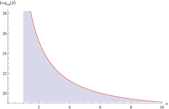
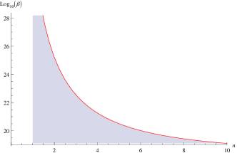
Figure 4: The lower bound of the chameleon–matter coupling constant $\beta$ from the experiments on the electron–neutron scattering length for the scattering of the slow neutron by lead (left) and bismuth (right), respectively. The shaded area is excluded.

The minimal lower bound $\beta\geq 10^{19}$ is ten orders of magnitude larger compared to the value $\beta<5.8\times 10^{8}$, measured recently in the qBounce experiments Jenke2014 . As a result, the contribution of the chameleon field to the electron–scattering length in the environment of the liquid lead and bismuth is negligible. Thus, in order to obtain a tangible contribution of the chameleon to the electron–neutron scattering length $b_{ne}$ or the squared charge radius of the neutron $r^{2}_{n}$, the experiments should be carried out in the environments with densities of order $\rho\sim 10^{-7}\,{\rm g/cm^{3}}$ or even smaller.

VII.2 Contributions of the chameleon field to the squared charge radius of the proton $r^{2}_{p}$

The results obtained above for the squared charge radius of the neutron can be applied to the analysis of the contribution of the chameleon (torsion) to the squared charge radius of the proton. Since the interaction of the chameleon field with the proton is described by the Lagrangian Eq.(105) with the replacement $n(x)\to p(x)$, where $p(x)$ is the operator of the proton field, the contribution of the chameleon field to the squared charge radius of the proton $r^{2}_{p}$ is defined by Eqs.(113) and (45) with the replacement $r^{2}_{n}\to\delta r^{2}_{p}$, $m_{n}\to m_{p}$ and $m_{e}\to m_{\mu}$, where $m_{\mu}$ is the mass of the $\mu^{-}$–meson PDG2014 .

The contribution of the chameleon field to the charge radius of the proton has been recently investigated by Brax and Burrage Brax2014 . According to Brax and Burrage Brax2014 , the contribution of the chameleon field may solve the so–called “the proton radius anomaly” Pohl2010 ; Batell2011 ; Pohl2013 ; Pohl2014 . As has been shown in Pachucki1996 –Matynenko2008 the Lamb shift $\Delta E_{2s\to 2p}$ of the muonic hydrogen, calculated in QED with the account for the nuclear effects, can be expressed in terms of the charge radius of the proton $r_{p}$

$$\Delta E_{2s\to 2p}=209.9779(49)-5.2262\,r^{2}_{p}+0.0347\,r^{3}_{p},$$ (117)

where $\Delta E_{2s\to 2p}$ and $r_{p}$ are measured in ${\rm meV}$ and ${\rm fm}$, respectively. The charge radius of the proton $r_{p}=0.8768(69)\,{\rm fm}$, measured from the electronic hydrogen Mohr2008 and agreeing well with the charge radius of the proton $r_{p}=0.879(8)\,{\rm fm}$, extracted from in the electron scattering experiments Bernauer2010 . In turn, the experimental value of the charge proton radius $r_{p}=0.84087(39)\,{\rm fm}$, extracted from the measurements of the Lamb shift of muonic hydrogen Antognini2013 , is of about $4\,\%$ smaller compared to the charge radius of the proton, measured from the electronic hydrogen Batell2011 . The correction to the Lamb shift, caused by the correction to the squared charge radius $\delta r^{2}_{p}$, is equal to

$$\delta E_{2s\to 2p}=(-5.2262+0.0521\,r_{p})\,\delta r^{2}_{p}=-5.180\,\delta r^{2}_{p},$$ (118)

where we have set $r_{p}=0.8768\,{\rm fm}$. The correction to the charge radius of the proton, caused by low energy $\mu\,p$ scattering, is equal to (see Eq.(113))

$$\delta r^{2}_{p}=-\frac{9}{4\pi^{2}}\,\frac{\beta^{2}}{m^{2}_{\phi}}\,\frac{m_{\mu}m_{p}}{M^{2}_{\rm Pl}}{\ell n}\Big{(}\frac{M_{\rm Pl}}{m_{\mu}}\Big{)}=-6.617\times 10^{-15}\,\frac{\beta^{2}}{m^{2}_{\phi}},$$ (119)

where $m_{\mu}=105.6584\,{\rm MeV}$ and $m_{p}=938.2720\,{\rm MeV}$ are the muon and proton masses, respectively PDG2014 , and $m_{\phi}$ and $\delta r^{2}_{p}$ are measured in ${\rm meV}$ and ${\rm fm^{2}}$, respectively. Substituting Eq.(119) into Eq.(118) we express the correction to the Lamb shift of the muonic hydrogen in terms of the parameters of the chameleon field theory and the matter density $\rho_{m}$. We get

$$\delta E_{2s\to 2p}=3.428\times 10^{-14}\,\frac{\beta^{2}}{m^{2}_{\phi}}=5.951\times 10^{-15}\,\frac{\beta^{\textstyle\frac{n}{n+1}}}{n((n+1)}\,\Big{(}\frac{nM_{\rm Pl}\Lambda^{3}}{\rho_{m}}\Big{)}^{\textstyle\frac{n+2}{n+1}}$$ (120)

with $\delta E_{2s\to 2p}=0.311\,{\rm meV}$ Pohl2014 . In Fig. 5 we plot the coupling constant $\beta$ as a function of the Ratra–Peebles index $n$ at the environment density $\rho_{m}\approx 10\,{\rm g/cm^{3}}$ Chameleon1 . One may see that for $\delta E_{2s\to 2p}=0.311\,{\rm meV}$ the lower bound of the chameleon–matter coupling constant $\beta$, at which the contribution of the chameleon is tangible, is $\beta\geq 10^{16}$. This is seven orders of magnitude larger compared to the recent experimental upper bound $\beta<5.8\times 10^{8}$ Jenke2014 .

Figure 5: The chameleon–matter coupling constant $\beta$ as a function of the index $n$, fitting the experimental value $\delta E_{2s-2p}=\Delta E_{2s-2p}-\Delta E_{2s-2p}|_{r_{p}=0.8768}=0.311\,{\rm meV}$, where $\Delta E_{2s-2p}=206.2949\,{\rm meV}$ Pohl2010 , of the Lamb shift of muonic hydrogen Pohl2014 .The shaded area is excluded.

VII.3 Contribution of the chameleon field to the neutron $\beta^{-}$–decay

In this section we investigate the neutron $\beta^{-}$–decay, caused by the interaction with the chameleon. This means that we investigate two reactions: i) the neutron $\beta^{-}$–decay with an emission of the chameleon $n\to p+e^{-}+\bar{\nu}_{e}+\phi$ and ii) the chameleon induced neutron $\beta^{-}$–decay $\phi+n\to p+e^{-}+\bar{\nu}_{e}$. Since formally these two reactions are related by $k_{\phi}\to-k_{\phi}$, where $k_{\phi}$ is a 4–momentum of the chameleon, we give the calculation of the amplitude of the neutron $\beta^{-}$–decay $n\to p+e^{-}+\bar{\nu}_{e}+\phi$ with an emission of the chameleon.

Neutron $\beta^{-}$–decay with the chameleon particle in the final state $n\to p+e^{-}+\bar{\nu}_{e}+\phi$

The calculation of the amplitude of such a decay we use the following effective interactions

$${\cal L}_{\rm eff} = -\beta\,\frac{m_{n}}{M_{\rm Pl}}\,\bar{n}(x)n(x)\,\phi(x)-\beta\,\frac{m_{p}}{M_{\rm Pl}}\,\bar{p}(x)p(x)\,\phi(x)$$ (121)

$$-\frac{G_{F}}{\sqrt{2}}\,V_{ud}\,\Big{\{}[\bar{p}(x)\gamma_{\mu}(1+\lambda\gamma^{5})n(x)]+\frac{\kappa}{2M}\partial^{\nu}[\bar{p}(x)\sigma_{\mu\nu}n(x)]\Big{\}}[\bar{e}^{-}(x)\gamma^{\mu}(1-\gamma^{5})\nu_{e}(x)],$$

where $G_{F}=1.1664\times 10^{-1}\,{\rm MeV^{-2}}$ is the Fermi coupling constant, $V_{ud}=0.97427(15)$ is the Cabibbo–Kobayashi–Maskawa (CKM) quark mixing matrix element PDG2014 , $\lambda=-1.2750(9)$ is the axial coupling constant Abele2008 (see alsoIvanov2013a ) and $\kappa=\kappa_{p}-\kappa_{n}=3.7058$ is the isovector anomalous magnetic moment of the nucleon, defined by the anomalous magnetic moments of the proton $\kappa_{p}=1.7928$ and the neutron $\kappa_{n}=-1.9130$ and measured in nuclear magneton PDG2014 , $M=(m_{n}+m_{p})/2$ is the nucleon average mass.

The Feynman diagrams of the amplitude of the neutron $\beta^{-}$–decay $n\to p+e^{-}+\bar{\nu}_{e}+\phi$ are shown in Fig. 6. For the calculation of the analytical expression of the decay amplitude we follow Ivanov2013a and carry out it in the rest frame of the neutron, keeping the contributions of the terms to order $1/M$. The energy spectrum and angular distribution of the neutron $\beta^{-}$–decay with polarised neutron and unpolarised proton and electron we may write in the following general form

$$\frac{d^{12}\lambda_{n\phi}}{d\Gamma^{12}}=\frac{G^{2}_{F}|V_{ud}|^{2}}{4m_{n}}\beta^{2}\frac{M^{2}}{M^{2}_{\rm Pl}}\overline{|M(n\to p\,e^{-}\,\bar{\nu}_{e}\,\phi)|^{2}}\,F(E_{e},Z=1)\,\Phi(\vec{k}_{e},\vec{k}_{\nu},\vec{k}_{\phi})\,(2\pi)^{4}\,\delta^{(4)}(k_{n}-k_{p}-k_{e}-k_{\nu}-k_{\phi}),$$ (122)

where $F(E_{e},Z=1)$ is the relativistic Fermi function, describing the final–state electron–proton Coulomb interaction Ivanov2013 , $d^{12}\Gamma$ is the phase–volume of the decay final state

$$d\Gamma^{12}=\frac{d^{3}k_{p}}{(2\pi)^{3}2E_{p}}\frac{d^{3}k_{e}}{(2\pi)^{3}2E_{e}}\frac{d^{3}k_{\nu}}{(2\pi)^{3}2E_{\nu}}\frac{d^{3}k_{\phi}}{(2\pi)^{3}2E_{\phi}}$$ (123)

and $k_{j}$ for $j=n,p,e,\nu$ and $\phi$ is a 4–momentum of the neutron and the decay particles, respectively. The factor $\Phi(\vec{k}_{e},\vec{k}_{\nu},\vec{k}_{\phi})$ is the contribution of the phase–volume, taking into account the terms of order $1/M$. Following Ivanov2013a one obtains

$$\Phi(\vec{k}_{e},\vec{k}_{\nu},\vec{k}_{\phi})=1+\frac{3}{M}\Big{(}E_{e}-\frac{\vec{k}_{e}\cdot\vec{k}_{\nu}}{E_{\nu}}\Big{)}+\frac{3}{M}\Big{(}E_{\phi}-\frac{\vec{k}_{\phi}\cdot\vec{k}_{\nu}}{E_{\nu}}\Big{)}+\frac{2}{M}\,\frac{E_{e}E_{\phi}-\vec{k}_{e}\cdot\vec{k}_{\phi}}{E_{\nu}}.$$ (124)

The last two terms define the deviation from the phase–volume factor, calculated in Ivanov2013a for the neutron $\beta^{-}$–decay $n\to p+e^{-}+\bar{\nu}_{e}$. Taking into account the phase–volume factor $\Phi(\vec{k}_{e},\vec{k}_{\nu},\vec{k}_{\phi})$ we may carry out the integration over the phase–volume of the $n\to p+e^{-}+\bar{\nu}_{e}+\phi$ decay, neglecting the contribution of the kinetic energy of the proton.

Then, $\overline{|M(n\to p\,e^{-}\,\bar{\nu}_{e}\,\phi)|^{2}}$ is the squared absolute value of the decay amplitude, summed over the polarisation of the decay electron and proton.

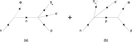
Figure 6: Feynman diagrams of the neutron $\beta^{-}$–decay with an emission of the chameleon $n\to p+e^{-}+\bar{\nu}_{e}+\phi$.

The analytical expression of the amplitude $M(n\to p\,e^{-}\,\bar{\nu}_{e}\,\phi)$ is defined by

$$M(n\to p\,e^{-}\,\bar{\nu}_{e}\,\phi) = \Big{[}\bar{u}_{p}(k_{p},\sigma_{p})\,\frac{1}{m_{p}-\hat{k}_{p}+\hat{k}_{\phi}-i0}\,O^{(-)}_{\mu}\,u_{n}(k_{n},\sigma_{n})\Big{]}\Big{[}\bar{u}_{e}(k_{e},\sigma_{e})\gamma^{\mu}(1-\gamma^{5})v_{\bar{\nu}_{e}}(k_{\nu},+\frac{1}{2})\Big{]}$$ (125)

$$+ \Big{[}\bar{u}_{p}(k_{p},\sigma_{p})\,O^{(+)}_{\mu}\,\frac{1}{m_{n}-\hat{k}_{n}+\hat{k}_{\phi}-i0}u_{n}(k_{n},\sigma_{n})\Big{]}\Big{[}\bar{u}_{e}(k_{e},\sigma_{e})\gamma^{\mu}(1-\gamma^{5})v_{\bar{\nu}_{e}}(k_{\nu},+\frac{1}{2})\Big{]},$$

where $u_{j}(k_{j},\sigma_{j})$ for $j=n,p$ and $e$ are the Dirac bispinors of fermions with polarisations $\sigma_{j}$, $v_{\bar{\nu}_{e}}(k_{\nu},+1/2)$ is the Dirac bispinor of the electron antineutrino and $O_{\mu}$ is defined by Ivanov2013a

$$O^{(\pm)}_{\mu}(k_{p},k_{n})=\gamma_{\mu}(1+\lambda\gamma^{5})+i\,\frac{\kappa}{2M}\,\sigma_{\mu\nu}(k_{p}-k_{n}\pm k_{\phi})^{\nu}.$$ (126)

In the accepted approximation the amplitude Eq.(124) can be defined by the expression

$$M(n\to p\,e^{-}\,\bar{\nu}_{e}\,\phi) = \frac{2}{E_{\phi}}\,[\bar{u}_{p}(k_{p},\sigma_{p})\,{\cal O}_{\mu}u_{n}(k_{n},\sigma_{n})]\Big{[}\bar{u}_{e}(k_{e},\sigma_{e})\gamma^{\mu}(1-\gamma^{5})v_{\bar{\nu}_{e}}(k_{\nu},+\frac{1}{2})\Big{]}=$$ (127)

$$= \frac{2}{E_{\phi}}[\bar{u}_{p}(k_{p},\sigma_{p})\,{\cal O}_{0}u_{n}(k_{n},\sigma_{n})]\Big{[}\bar{u}_{e}(k_{e},\sigma_{e})\gamma^{0}(1-\gamma^{5})v_{\bar{\nu}_{e}}(k_{\nu},+\frac{1}{2})\Big{]}$$

$$- \frac{2}{E_{\phi}}[\bar{u}_{p}(k_{p},\sigma_{p})\,\vec{{\cal O}}\,u_{n}(k_{n},\sigma_{n})]\cdot\Big{[}\bar{u}_{e}(k_{e},\sigma_{e})\vec{\gamma}\,(1-\gamma^{5})v_{\bar{\nu}_{e}}(k_{\nu},+\frac{1}{2})\Big{]}$$

where ${\cal O}_{\mu}$ is given by

$${\cal O}_{\mu}=\gamma_{\mu}(1+\lambda\gamma^{5})+i\,\frac{\kappa}{2M}\,\sigma_{\mu\nu}(k_{p}-k_{n})^{\nu}-\frac{k_{\phi\mu}}{2M}-i\,\frac{\lambda}{2M}\,\sigma_{\mu\nu}\gamma^{5}k^{\nu}_{\phi}$$ (128)

and the matrices ${\cal O}_{0}$ and $\vec{{\cal O}}$, taken to order $1/M$, are equal to

$$O^{0}=\left(\begin{array}[]{ccc}1-{\displaystyle\frac{E_{\phi}}{2M}+\frac{\lambda}{2M}\,(\vec{\sigma}\cdot\vec{k}_{\phi})}&{\displaystyle\lambda+\frac{\kappa}{2M}\,(\vec{\sigma}\cdot\vec{k}_{p})}\\ {\displaystyle-\lambda+\frac{\kappa}{2M}\,(\vec{\sigma}\cdot\vec{k}_{p})}&-1-{\displaystyle\frac{E_{\phi}}{2M}+\frac{\lambda}{2M}\,(\vec{\sigma}\cdot\vec{k}_{\phi})}\\ \end{array}\right)$$ (131)

and

$$\vec{O}=\left(\begin{array}[]{ccc}{\displaystyle\lambda\vec{\sigma}\Big{(}1-\frac{E_{\phi}}{2M}\Big{)}-\frac{\vec{k}_{\phi}}{2M}+i\,\frac{\kappa}{2M}\,(\vec{\sigma}\times\vec{k}_{p})}&{\displaystyle\vec{\sigma}\,\Big{(}1-\frac{\kappa}{2M}\,E_{0}\Big{)}-i\,\frac{\lambda}{2M}\,(\vec{\sigma}\times\vec{k}_{\phi})}\\ {\displaystyle-\,\vec{\sigma}\,\Big{(}1+\frac{\kappa}{2M}\,E_{0}\Big{)}-i\,\frac{\lambda}{2M}\,(\vec{\sigma}\times\vec{k}_{\phi})}&{\displaystyle-\lambda\vec{\sigma}\Big{(}1+\frac{E_{\phi}}{2M}\Big{)}-\frac{\vec{k}_{\phi}}{2M}+i\frac{\kappa}{2M}\,(\vec{\sigma}\times\vec{k}_{p})}\\ \end{array}\right),$$ (134)

where $E_{0}=((m_{n}-m_{\phi})^{2}-m^{2}_{p}+m^{2}_{e})/2(m_{n}-m_{\phi})$ is the end–point energy of the electron–energy spectrum. The matrices $O^{0}$ and $\vec{O}$ are defined to order $1/M$ only Ivanov2013a . For the calculation of the amplitude of the $\beta^{-}$–decay of the neutron we use the Dirac bispinorial wave functions of the neutron and the proton

$$u_{n}(\vec{0},\sigma_{n})=\sqrt{2m_{n}}\Big{(}\begin{array}[]{c}\varphi_{n}\\ 0\end{array}\Big{)}\quad,\quad u_{p}(\vec{k}_{p},\sigma_{p})=\sqrt{E_{p}+m_{p}}\left(\begin{array}[]{c}\varphi_{p}\\ {\displaystyle\frac{\vec{\sigma}\cdot\vec{k}_{p}}{E_{p}+m_{p}}\,\varphi_{p}}\end{array}\right),$$ (140)

where $\varphi_{n}$ and $\varphi_{p}$ are the Pauli spinor functions of the neutron and proton, respectively. For the energy spectrum and angular distribution of the neutron $\beta^{-}$–decay with polarised neutron and unpolarised proton and electron we may write in the following general form

$$\frac{d^{12}\lambda_{n\phi}}{d\Gamma^{12}}=32\,m_{p}\,E_{e}E_{\nu}\,\frac{G^{2}_{F}|V_{ud}|^{2}}{E^{2}_{\phi}}\beta^{2}\frac{M^{2}}{M^{2}_{\rm Pl}}\,F(E_{e},Z=1)\,(2\pi)^{4}\,\delta^{(4)}(k_{n}-k_{p}-k_{e}-k_{\nu}-k_{\phi})\,(1+3\lambda^{2})\,\zeta(E_{e})$$

$$\times\,\Big{\{}1+a(E_{e})\,\frac{\vec{k}_{e}\cdot\vec{k}_{\nu}}{E_{e}E_{\nu}}+A(E_{e})\,\frac{\vec{\xi}_{n}\cdot\vec{k}_{e}}{E_{e}}+B(E_{e})\,\frac{\vec{\xi}_{n}\cdot\vec{k}_{\nu}}{E_{\nu}}+K_{n}(E_{e})\,\frac{(\vec{\xi}_{n}\cdot\vec{k}_{e})(\vec{k}_{e}\cdot\vec{k}_{\nu})}{E^{2}_{e}E_{\nu}}+Q_{n}(E_{e})\,\frac{(\vec{\xi}_{n}\cdot\vec{k}_{\nu})(\vec{k}_{e}\cdot\vec{k}_{\nu})}{E_{e}E^{2}_{\nu}}$$

$$+D(E_{e})\,\frac{\vec{\xi}_{n}\cdot(\vec{k}_{e}\times\vec{k}_{\nu})}{E_{e}E}-3\,\frac{1-\lambda^{2}}{1+3\lambda^{2}}\,\frac{E_{e}}{M}\,\Big{(}\frac{(\vec{k}_{e}\cdot\vec{k}_{\nu})^{2}}{E^{2}_{e}E^{2}_{\nu}}-\frac{1}{3}\,\frac{k^{2}_{e}}{E^{2}_{e}}\,\Big{)}+\frac{1}{M}\,\frac{1}{1+3\lambda^{2}}\,F_{\phi}\Big{\}},$$ (141)

where $k_{e}=\sqrt{E^{2}_{e}-m^{2}_{e}}$ is the absolute value of the electron 3–momentum and $\vec{\xi}_{n}$ is the unit polarisation vector of the neutron $|\vec{\xi}_{n}|=1$. The correlation coefficients $\zeta(E_{e})$, $a(E_{e})$, $A(E_{e})$, $B(E_{e})$, $K_{n}(E_{e})$, $Q_{n}(E_{e})$ and $D(E_{e})$ can taken from Ivanov2013a at the neglect of the radiative corrections. The correction coefficient $F_{\phi}$ we may represent in the following form

$$F_{\phi}=F^{(1)}_{\phi}+F^{(2)}_{\phi}+F^{(3)}_{\phi},$$ (142)

where the correlation coefficients $F^{(j)}_{\phi}$ for $j=1,2,3$ are defined by i) the contributions of the terms, depending on the energy and 3–momentum of the chameleon particle in the matrices ${\cal O}_{0}$ and $\vec{\cal O}$ given by Eqs.(128) and (131), ii) the dependence of the 3–momentum of the proton $\vec{k}_{p}$ on the 3–momentum of the chameleon particle, caused by the 3–momentum conservation $\vec{k}_{p}=-\vec{k}_{e}-\vec{k}_{\nu}-\vec{k}_{\phi}$ (see Eqs.(A.16) and (A.17) in Appendix A of Ref.Ivanov2013a ) and iii) the contributions of the phase–volume factor Eq.(124), respectively. The analytical expressions of these correlation coefficients are equal to

$$F^{(1)}_{\phi} = (1+3\lambda^{2})\,E_{\phi}-(1-\lambda^{2})\,E_{\phi}\,\frac{\vec{k}_{e}\cdot\vec{k}_{\nu}}{E_{e}E_{\nu}}+2\,\lambda^{2}\,E_{\phi}\,\frac{\vec{\xi}_{n}\cdot\vec{k}_{e}}{E_{e}}-2\,\lambda^{2}\,E_{\phi}\,\frac{\vec{\xi}_{n}\cdot\vec{k}_{\nu}}{E_{\nu}}$$ (143)

$$+ 2\,\lambda\,\frac{(\vec{\xi}_{n}\cdot\vec{k}_{\phi})(\vec{k}_{e}\cdot\vec{k}_{\nu})}{E_{e}E_{\nu}}-\lambda\,\frac{(\vec{\xi}_{n}\cdot\vec{k}_{e})(\vec{k}_{\nu}\cdot\vec{k}_{\phi})}{E_{e}E_{\nu}}-\lambda\,\frac{(\vec{\xi}_{n}\cdot\vec{k}_{\nu})(\vec{k}_{e}\cdot\vec{k}_{\phi})}{E_{e}E_{\nu}},$$

$$F^{(2)}_{\phi} = (\lambda^{2}-2(\kappa+1)\,\lambda)\,\frac{\vec{k}_{e}\cdot\vec{k}_{\phi}}{E_{e}}+(\lambda^{2}+2(\kappa+1)\,\lambda)\,\frac{\vec{k}_{\nu}\cdot\vec{k}_{\phi}}{E_{\nu}}+(2\kappa+1)\,\lambda\,(\vec{\xi}_{n}\cdot\vec{k}_{\phi})-\lambda\,\frac{(\vec{\xi}_{n}\cdot\vec{k}_{\phi})(\vec{k}_{e}\cdot\vec{k}_{\nu})}{E_{e}E_{\nu}}$$ (144)

$$- (\lambda^{2}+(\kappa+1)\,\lambda+(\kappa+1))\,\frac{(\vec{\xi}_{n}\cdot\vec{k}_{e})(\vec{k}_{\nu}\cdot\vec{k}_{\phi})}{E_{e}E_{\nu}}+(\lambda^{2}-(\kappa+1)\lambda+(\kappa+1))\,\frac{(\vec{\xi}_{n}\cdot\vec{k}_{\nu})(\vec{k}_{e}\cdot\vec{k}_{\phi})}{E_{e}E_{\nu}}$$

and

$$F^{(3)}_{\phi}=\Big{[}3\,\Big{(}E_{\phi}-\frac{\vec{k}_{\phi}\cdot\vec{k}_{\nu}}{E_{\nu}}\Big{)}+2\,\frac{E_{e}E_{\phi}-\vec{k}_{e}\cdot\vec{k}_{\phi}}{E_{\nu}}\Big{]}\Big{[}(1-\lambda^{2})\,\frac{\vec{k}_{e}\cdot\vec{k}_{\nu}}{E_{e}E_{\nu}}-2\lambda(1+\lambda)\,\frac{\vec{\xi}_{n}\cdot\vec{k}_{e}}{E_{e}}-2\lambda(1-\lambda)\,\frac{\vec{\xi}_{n}\cdot\vec{k}_{\nu}}{E_{\nu}}\Big{]}.$$ (145)

Now we may integrate over the phase–volume of the $n\to p+e^{-}+\bar{\nu}_{e}+\phi$ decay. First of all we integrate over the 3–momentum of the proton $\vec{k}_{p}$. As has been mention above, we make such an integration at the neglect of the kinetic energy of the proton. Then, since one can hardly observe the dependence of the energy spectrum and the angular distribution on the direction of the 3–momentum of the chameleon, we make the integration over the 3–momentum of the chameleon $\vec{k}_{\phi}$. The obtained energy spectrum and angular distribution is

$$\frac{d^{7}\lambda_{n\phi}(E_{e},E_{\nu},E_{\phi},\vec{k}_{e},\vec{k}_{\nu},\vec{\xi}_{n})}{dE_{e}dE_{\nu}dE_{\phi}d\Omega_{e}d\Omega_{\nu}}=\frac{G^{2}_{F}|V_{ud}|^{2}}{32\pi^{7}E_{\phi}}\beta^{2}\frac{M^{2}}{M^{2}_{\rm Pl}}\,F(E_{e},Z=1)\,\delta(E_{0}-E_{e}-E_{\nu}-E_{\phi})\,k_{e}E_{e}\,E^{2}_{\nu}\,(1+3\lambda^{2})\,\zeta_{\phi}(E_{e})$$

$$\times\,\Big{\{}1+a_{\phi}(E_{e})\,\frac{\vec{k}_{e}\cdot\vec{k}_{\nu}}{E_{e}E_{\nu}}+A_{\phi}(E_{e})\,\frac{\vec{\xi}_{n}\cdot\vec{k}_{e}}{E_{e}}+B_{\phi}(E_{e})\,\frac{\vec{\xi}_{n}\cdot\vec{k}_{\nu}}{E_{\nu}}+K_{n}(E_{e})\,\frac{(\vec{\xi}_{n}\cdot\vec{k}_{e})(\vec{k}_{e}\cdot\vec{k}_{\nu})}{E^{2}_{e}E_{\nu}}+Q_{n}(E_{e})\,\frac{(\vec{\xi}_{n}\cdot\vec{k}_{\nu})(\vec{k}_{e}\cdot\vec{k}_{\nu})}{E_{e}E^{2}_{\nu}}$$

$$+D(E_{e})\,\frac{\vec{\xi}_{n}\cdot(\vec{k}_{e}\times\vec{k}_{\nu})}{E_{e}E_{\nu}}-3\,\frac{1-\lambda^{2}}{1+3\lambda^{2}}\,\frac{E_{e}}{M}\,\Big{(}\frac{(\vec{k}_{e}\cdot\vec{k}_{\nu})^{2}}{E^{2}_{e}E^{2}_{\nu}}-\frac{1}{3}\,\frac{k^{2}_{e}}{E^{2}_{e}}\,\Big{)}\Big{\}}.$$ (146)

The correlation coefficients $\zeta_{\phi}(E_{e})$, $a_{\phi}(E_{e})$, $A_{\phi}(E_{e})$ and $B_{\phi}(E_{e})$ are equal to

$$\zeta_{\phi}(E_{e}) = \bar{\zeta}(E_{e})+\frac{E_{\phi}}{M},$$

$$a_{\phi}(E_{e}) = \bar{a}(E_{e})+a_{0}\,\Big{(}1+2\,\frac{E_{e}}{E_{\nu}}\Big{)}\,\frac{E_{\phi}}{M}$$

$$A_{\phi}(E_{e}) = \bar{A}(E_{e})+\Big{(}-2\lambda+A_{0}\,\Big{(}1+2\,\frac{E_{e}}{E_{\nu}}\Big{)}\Big{)}\,\frac{E_{\phi}}{M},$$

$$B_{\phi}(E_{e}) = \bar{B}(E_{e})+\Big{(}-2\lambda+B_{0}\,\Big{(}1+2\,\frac{E_{e}}{E_{\nu}}\Big{)}\Big{)}\,\frac{E_{\phi}}{M},$$ (147)

where $a_{0}=(1-\lambda^{2})/(1+3\lambda^{2})$, $A_{0}=-2\lambda(1+\lambda)/(1+3\lambda^{2})$ and $B_{0}=-2\lambda(1-\lambda)/(1+3\lambda^{2})$ Abele2008 (see also Ivanov2013a ). The correlation coefficients $\bar{\zeta}(E_{e})$, $\bar{a}(E_{e})$, $\bar{A}(E_{e})$ and $\bar{B}(E_{e})$ are calculated in Ivanov2013a by taking into account the contributions of the weak magnetism and the proton recoil to order $1/M$ but without radiative corrections.

The rate of the decay $n\to p+e^{-}+\bar{\nu}_{e}+\phi$ diverges logarithmically at $E_{\phi}\to 0$. We regularise the logarithmically divergent integral by the chameleon mass $m_{\phi}$. As result we get

$$\lambda_{n\phi}=\frac{G^{2}_{F}|V_{ud}|^{2}}{2\pi^{3}}\,\frac{\beta^{2}}{\pi^{2}}\,\frac{M^{2}}{M^{2}_{\rm Pl}}\,f_{\phi}(E_{0},Z=1),$$ (148)

where $f_{\phi}(E_{0},Z=1)$ is the Fermi integral

$$f_{\phi}(E_{0},Z=1)=\int^{E_{0}}_{m_{e}}dE_{e}\,E_{e}\,\sqrt{E^{2}_{e}-m^{2}_{e}}\,(E_{0}-E_{e})^{2}\Big{[}{\ell n}\Big{(}\frac{E_{0}-E_{e}}{m_{\phi}}\Big{)}-\frac{3}{2}+\frac{1}{3}\,\frac{E_{0}-E_{e}}{M}\Big{]}\,\bar{\zeta}(E_{e})\,F(E_{e},Z=1),$$ (149)

where $\bar{\zeta}(E_{e})$ is given by (see Eq.(7) of Ref.Ivanov2013a )

$$\bar{\zeta}(E_{e})=1+\frac{1}{M}\,\frac{1}{1+3\lambda^{2}}\,\Big{[}-2\,\lambda\Big{(}\lambda-(\kappa+1)\Big{)}\,E_{0}+\Big{(}10\lambda^{2}-4(\kappa+1)\,\lambda+2\Big{)}\,E_{e}-2\lambda\,\Big{(}\lambda-(\kappa+1)\Big{)}\,\frac{m^{2}_{e}}{E_{e}}\Big{]}.$$ (150)

In Fig. 7 we plot the electron–energy spectrum $\rho_{\phi}(E_{e})$ of the neutron $\beta^{-}$–decay with an emission of the chameleon, defined by

$$\rho_{\phi}(E_{e})=E_{e}\,\sqrt{E^{2}-m^{2}_{e}}\,(E_{0}-E_{e})^{2}\Big{[}{\ell n}\Big{(}\frac{E_{0}-E_{e}}{m_{\phi}}\Big{)}-\frac{3}{2}+\frac{1}{3}\,\frac{E_{0}-E_{e}}{M}\Big{]}\,\bar{\zeta}(E_{e})\,\frac{F(E_{e},Z=1)}{f(E_{0},Z=1)},$$ (151)

where $f(E_{0},Z=1)$ is the Fermi integral calculated in Ivanov2013a , and compare it with the electron–energy spectrum $\rho_{\beta^{-}_{c}}(E_{e})$ of the neutron $\beta^{-}$–decay calculated in Ivanov2013a (see Eq.(D-59) of Ref.Ivanov2013a ). The chameleon mass $m_{\phi}$ is determined at the local density $\rho\simeq 1.19\times 10^{-11}\,{\rm g/cm^{3}}=5.12\times 10^{-17}\,{\rm MeV^{4}}$. This is the density of air at room temperature and pressure $P\simeq 10^{-5}\,{\rm mbar}$ Serebrov2008 ; Pichlmaier2010 . For $\beta<5.8\times 10^{8}$ we obtain $\lambda_{n\phi}<2\times 10^{-34}\,{\rm s^{-1}}$ and the branching ratio ${\rm BR}_{n\phi}<1.8\times 10^{-31}$.

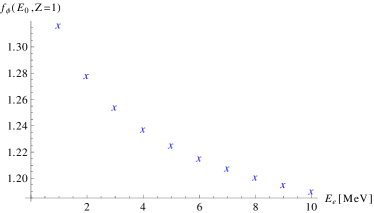
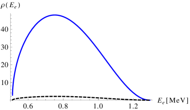
Figure 7: (left) The values of the Fermi integral $f_{\phi}(E_{0},Z=1)$ as a function of the index $n$ for $n=1,2,\ldots,10$. (right) The electron–energy spectra $\rho_{\phi}(E_{e})$ (continuous lines) and $\rho_{\beta^{-}_{c}}(E_{e})$ (dashed line) of the neutron $\beta^{-}$–decay with and without an emission of a chameleon, respectively. The densities $\rho_{\phi}(E_{e})$ depend slightly on the index $n$ and are represented by only one continuous blue line.

Neutron $\beta^{-}$–decay $\phi+n\to p+e^{-}+\bar{\nu}_{e}$, induced by the chameleon field

For the calculation of the amplitude $M(\phi\,n\to p\,e^{-}\,\bar{\nu}_{e})$ of the induced neutron $\beta^{-}$–decay $\phi+n\to p+e^{-}+\bar{\nu}_{e}$ we may use the amplitude Eq.(125) with the replacement $k_{\phi}\to-k_{\phi}$, where $k_{\phi}$ is a 4–momentum of the chameleon. The Feynman diagrams for the chameleon–induced neutron $\beta^{-}$–decay is shown in Fig. 8.

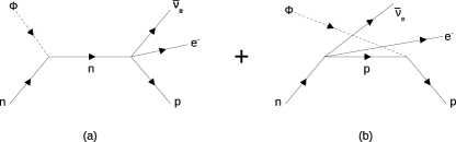
Figure 8: Feynman diagrams for the reaction $\phi+n\to p+e^{-}+\bar{\nu}_{e}$

The cross section for the induced neutron $\beta^{-}$–decay is

$$\sigma_{\phi\,n\to p\,e^{-}\,\bar{\nu}_{e}}(E_{\phi})=\frac{1}{4m_{n}E_{\phi}}\int\overline{|M(\phi\,n\to p\,e^{-}\,\bar{\nu}_{e})|^{2}}\,(2\pi)^{4}\,\delta^{(4)}(k_{n}+k_{\phi}-k_{p}-k_{e}-k_{\nu})\,\frac{d^{3}k_{p}}{(2\pi)^{3}2E_{p}}\frac{d^{3}k_{e}}{(2\pi)^{3}2E_{e}}\frac{d^{3}k_{\nu}}{(2\pi)^{3}2E_{\nu}},$$

where the contribution of the electron–proton final–state Coulomb interaction is not important and neglected. Using the results, obtained in previous subsection, we get

$$\sigma_{\phi\,n\to p\,e^{-}\,\bar{\nu}_{e}}(E_{\phi})=(1+3\lambda^{2})\,\frac{G^{2}_{F}|V_{ud}|^{2}}{2\pi^{3}E^{3}_{\phi}}\,\beta^{2}\,\frac{M^{2}}{M^{2}_{\rm Pl}}\int^{E_{0}+E_{\phi}}_{m_{e}}dE_{e}\,E_{e}\,\sqrt{E^{2}-m^{2}_{e}}\,(E_{0}+E_{\phi}-E_{e})^{2}.$$ (153)

Integrating over $E_{e}$ we obtain

$$\sigma_{\phi\,n\to p\,e^{-}\,\bar{\nu}_{e}}(E_{\phi}) = (1+3\lambda^{2})\,\frac{G^{2}_{F}|V_{ud}|^{2}}{2\pi^{3}}\,\beta^{2}\,\frac{M^{2}}{M^{2}_{\rm Pl}}\frac{(E_{0}+E_{\phi})^{5}}{30E^{3}_{\phi}}\Bigg{\{}\Bigg{(}1-\frac{9}{2}\,\frac{m^{2}_{e}}{(E_{0}+E_{\phi})^{2}}-4\,\frac{m^{4}_{e}}{(E_{0}+E_{\phi})^{4}}\Bigg{)}$$ (154)

$$\times\sqrt{1-\frac{m^{2}_{e}}{(E_{0}+E_{\phi})^{2}}}+\frac{15}{2}\,\frac{m^{4}_{e}}{(E_{0}+E_{\phi})^{4}}\,{\ell n}\Bigg{(}\frac{E_{0}+E_{\phi}}{m_{e}}+\sqrt{\frac{(E_{0}+E_{\phi})^{2}}{m^{2}_{e}}-1}\;\Bigg{)}\Bigg{\}}.$$

Using the results, obtained in Brax2012 (see also Baum2014 ), we may analyse the quantity

$$\lambda_{\phi n}=\int^{\infty}_{0}dE_{\phi}\,\Phi_{\rm ch}(E_{\phi})\,\sigma_{\phi\,n\to p\,e^{-}\,\bar{\nu}_{e}}(E_{\phi}),$$ (155)

which defines the number of transitions $n\to p\,e^{-}\bar{\nu_{e}}$ per second, induced by the chameleon, where $\Phi_{\rm ch}(E_{\phi})$ is the number of solar chameleons per ${\rm eV\cdot s\cdot cm^{2}}$, normalised to $10\,\%$ of the solar luminosity per unite area $L_{\odot}/4\pi R_{\odot}=3.9305\times 10^{22}\,{\rm eV\,s^{-1}\,cm^{-2}}=0.01007\,{\rm eV^{4}}$ Brax2012 , where $L_{\odot}=2.3893\times 10^{45}\,{\rm eV\,s^{-1}}$ and $R_{\odot}=6.9551(4)\times 10^{10}\,{\rm cm}$ are the total luminosity and the radius of the Sun PDG2014 . Following Brax2012 we obtain that $\lambda_{\phi n}<10^{-41}\,{\rm s^{-1}}$ for $\beta<5.8\times 10^{8}$ Jenke2014 .

VIII Conclusion

We have developed the results, obtained in Ivanov2014 , where there was shown that the chameleon field can serve also as a source for a torsion field and low–energy torsion–neutron interactions, where the torsion field is determined by a gradient of the chameleon one. Following Hojman et al. Hojman1978 we have extended the Einstein gravitational theory with the chameleon field to a version of the Einstein–Cartan gravitational one with a torsion field. For the inclusion of the torsion field we have used a modified form of local gauge invariance in the Weinberg–Salam electroweak model with minimal coupling and derived the Lagrangians of the electroweak and gravitational interactions with the chameleon (torsion) field.

Gauge invariance of the torsion–photon interactions has been explicitly checked by calculating the amplitudes of the two–photon decay of the torsion (chameleon) field $\phi\to\gamma+\gamma$ and the photon–torsion (chameleon) scattering $\gamma+\phi\to\phi+\gamma$ or the Compton photon–torsion (chameleon) scattering. Unlike the Compton–scattering, where photons scatter by free charged particles with charged particles in the virtual intermediate states, in the photon–torsion (chameleon) scattering a transition from an initial $(\gamma\,\phi)$ state to a final $(\gamma\,\phi)$ goes through the one–virtual photon exchange (see Fig. 2a and Fig. 2b) and the local ${\cal L}_{\gamma\gamma\phi\phi}$ interaction (see Fig. 2c). The Feynman diagram Fig. 2d is self–gauge invariant due to the local ${\cal L}_{\gamma\gamma\phi}$ interaction. Gauge invariance has been checked directly by a replacement of the one of the polarisation vectors of the photons in the initial and final state by its 4-momentum. Since in these reactions the coupling constant of the photon–torsion (chameleon) interaction is $g_{\rm eff}=\beta/M_{\rm Pl}$, in analogy with gauge invariance of photon–charge particles interactions, where electric charge is a coupling constant - unrenormalisable by any interactions, one may assert that the coupling constant $g_{\rm eff}=\beta/M_{\rm Pl}$ should be also unrenormalisable by any interactions. This may place some strict constraints on possible mechanisms of the chameleon–matter coupling constant $\beta/M_{\rm Pl}$ screening Khoury2010 ; BraxCQG2013 . In this connection the Vainstein mechanism, leading the screening of the coupling constant $\beta/M_{\rm Pl}$ by the factor $1/\sqrt{Z}$, where $Z>1$ is a finite renormalisation constant of the wave function of the chameleon field caused by a self–interaction of the chameleon field BraxCQG2013 or some new higher derivative terms Bloomfield2014 , is prohibited in such a version of the Einstein–Cartan gravity with the chameleon field and torsion. Because of the smallness of the constant $\beta^{4}/M^{4}_{\rm Pl}<10^{-60}\,{\rm barn/eV^{2}}$, estimated for $\beta<5.8\times 10^{8}$ Jenke2014 , the cross section for the photon–chameleon scattering is extremely small and hardly may play any important cosmological role at low energies, for example, for a formation of the cosmological microwave background and so on. However, since in our approach the coupling constant $\beta_{\gamma}/M_{\rm Pl}$ is fixed in terms of the coupling constant $\beta/M_{\rm Pl}$, the recent measurement of the upper bound $\beta<5.8\times 10^{8}$ can make new constraints on the photon–chameleon oscillations in the magnetic field of the laboratory search for the chameleon field Steffen2010 ; Schelpe2010 ; Rybka2010 .

In our approach the effective chameleon–photon coupling $g_{\rm eff}=\beta/M_{\rm Pl}$ is equal to $g_{\rm eff}=\beta/M_{\rm Pl}<2.4\times 10^{-10}\,{\rm GeV^{-1}}$, where we have used the experimental upper bound of the chameleon–matter coupling constant $\beta<5.8\times 10^{8}$ Jenke2014 . The obtained upper bound $g_{\rm eff}<2.4\times 10^{-10}\,{\rm GeV^{-1}}$ is in qualitative agreement with the upper bounds, estimated by Davis, Schelpe and Shaw Davis2009 . Then, the constraints on $\beta$: $\beta<1.9\times 10^{7}\;(n=1)$, $\beta<5.8\times 10^{7}\;(n=2)$, $\beta<2.0\times 10^{8}\,(n=3)$ and $\beta<4.8\times 10^{8}\,(n=4)$, measured recently by H. Lemmel et al. Lemmel2015 using the neutron interferometer, may be used for more strict constraints on the astrophysical sources of chameleons, investigated in Brax2007 –Davis2009 .

Using the photon–torsion (chameleon) interaction we have estimated the contributions of the chameleon field to the charged radii of the neutron and proton. All tangible contributions can appear only for $\beta\gg 10^{8}$. This, of course, is not compatible with recent experimental data $\beta<5.8\times 10^{8}$ by Jenke et al. Jenke2014 . The branching ratio for the production of the chameleon in the neutron $\beta^{-}$–decay $n\to p+e^{-}+\bar{\nu}_{e}+\phi$ is extremely small ${\rm Br}(n\to p\,e^{-}\,\bar{\nu}_{e}\,\phi)<1.8\times 10^{-31}$. In turn, the half–life of the neutron $T^{(\phi\,n)}_{1/2}={\ell n}2/\lambda_{\phi n}$, caused by the chameleon induced neutron $\beta^{-}$–decay $\phi+n\to p+e^{-}+\bar{\nu}_{e}$, is extremely large $T^{(\phi\,n)}_{1/2}={\ell n}2/\lambda_{\phi n}>2\times 10^{33}\,{\rm yr}$. Of course, because of the neutron life–time $\tau_{n}=880.3(1.1)\,{\rm s}$ PDG2014 , being in agreement with the recent theoretical value $\tau_{n}=879.6(1.1)\,{\rm s}$ Ivanov2013a , the chameleon induced neutron $\beta^{-}$–decay cannot be observed by a free neutron. The experiment, which can give any meaningful result, can be organised in a way, which is used for the detection of the neutrinoless double $\beta$ decays Bahcall2004 . For example, it is known that the isotope ${{}^{76}}{\rm Ge}$ is both stable with respect to non–exotic weak, electromagnetic and nuclear decays and are neutron–rich. It is unstable only with respect to the neutrinoless double $\beta^{-}$–decay Bahcall2004 . The experimental analysis of the low–bound on the half–life of ${{}^{76}}{\rm Ge}$ has been carried out by the GERDA Collaboration Agostini et al. Gerda2013a ; Gerda2013b by measuring the energy spectrum of the electrons. The experimental lower bound has been found to be equal to $T_{1/2}>3\times 10^{25}\,{\rm yr}$ ($90\,\%\,{\rm C.L.}$). We would like also to mention the experiments on the proton decays, carried out by Super–Kamiokande SuperKamiokande2009 ; SuperKamiokande2014 . For specific modes of the proton decay, i.e. $p\to e^{+}\pi^{0}$, $p\to\mu^{+}\pi^{0}$ and $p\to\nu K^{+}$, for the half–life of the proton there have been found the following lower bounds: $T_{1/2}>5.7\times 10^{33}\,{\rm yr}$, $T_{1/2}>4.6\times 10^{33}\,{\rm yr}$ and $T_{1/2}>4.1\times 10^{33}\,{\rm yr}$, respectively.

Since the lifetime of the neutron $\tau_{n}=880.3(1.1)\,{\rm s}$ PDG2014 , one cannot analyse experimentally the chameleon–induced $\beta^{-}$–decay on free neutrons. For the experimental investigation of the chameleon–induced $\beta^{-}$–decay one may propose the following reaction

$$\phi+{{}^{112}_{~{}48}}{\rm Cd}\to{{}^{112}_{~{}49}}{\rm In}+e^{-}+\bar{\nu}_{e},$$ (156)

where ${{}^{112}_{~{}48}}{\rm Cd}$ is an atom with a stable nucleus in the ground state with spin^(parity) $J^{\pi}=0^{+}$. Since ${{}^{112}_{~{}49}}{\rm In}$ is an atom with a nucleus in the ground state with spin^(parity) $J^{\pi}=1^{+}$, the reaction Eq.(156) is determined by the Gamow–Teller transition ${{}^{112}_{~{}48}}{\rm Cd}\to{{}^{112}_{~{}49}}{\rm In}$ for chameleon energies $E_{\phi}\geq 3.088\,{\rm MeV}$. The calculation of the threshold energies in weak decay of heavy atoms with the account for the contribution of the electron shells can be found in Ivanov2008 .

We have to note that the atom ${{}^{112}_{~{}49}}{\rm In}$ is unstable under the electron capture (EC) and $\beta^{-}$ decays with the branches $56\,\%$ and $44\,\%$, respectively Tuli2005 . Since the EC decay of ${{}^{112}_{~{}49}}{\rm In}$ is not observable in the experiment on the chameleon–induced $\beta^{-}$–decay, one may observe the $\beta^{-}$–decay of ${{}^{112}_{~{}49}}{\rm In}$. However, the electron energy spectrum of ${{}^{112}_{~{}49}}{\rm In}$ is restricted by the end–point energy $E_{0}=0.673\,{\rm MeV}$ and can be distinguished from the energy spectrum of the electron, appearing in the final state of the reaction Eq.(156).

The main background for the chameleon–induced $\beta^{-}$–decay Eq.(156) is the reaction

$$\nu_{e}+{{}^{112}_{~{}48}}{\rm Cd}\to{{}^{112}_{~{}49}}{\rm In}+e^{-},$$ (157)

caused by solar neutrinos with energies $E_{\nu_{e}}\geq 3.088\,{\rm MeV}$. Because of the threshold energy the reaction Eq.(157) can be induced by only the solar ${{}^{8}}{\rm B}$ and hep neutrinos PDG2014 . Since the hep–solar neutrino flux is approximately 1000 times weaker in comparison to the ${{}^{8}}{\rm B}$–solar neutrino flux PDG2014 , the reaction Eq.(157) should be induced by the ${{}^{8}}{\rm B}$–solar neutrinos.

Concluding our analysis of standard electroweak interactions in the gravitational theory we would like to discuss the results, obtained recently by Obukhov et al. Obukhov2014 . There, the behaviour of the Dirac fermions in the Poincar$\acute{\rm e}$ gauge gravitational field including a torsion was analysed. The Hamilton operator of the spin–torsion interaction has been derived Obukhov2014 . In a weak gravitational field and torsion field approximation, which we develop in this paper, such a spin–torsion interaction takes the form

$${\rm H}_{\rm spin-tors}=-\frac{1}{4}\,(\vec{\Sigma}\cdot\vec{T}+\gamma^{5}T^{0}),$$ (158)

where $\vec{\Sigma}=\gamma^{0}\vec{\gamma}\gamma^{5}$ and $\gamma^{5}=i\gamma^{0}\gamma^{1}\gamma^{2}\gamma^{3}$ are the Dirac matrices Itzykson1980 . Then, $T^{0}$ and $\vec{T}$ are the time and spatial components of the axial torsion vector field $T^{\alpha}=(T^{0},\vec{T}\,)$, defined by

$$T^{\alpha}=-\frac{1}{2}\,\varepsilon^{\alpha\beta\mu\nu}\,{\cal T}_{\beta\mu\nu},$$ (159)

where ${\cal T}_{\beta\mu\nu}$ is the torsion tensor field and $\varepsilon^{\alpha\beta\mu\nu}$ is the totally antisymmetric Levi–Civita tensor $\varepsilon^{0123}=1$ Itzykson1980 . Using the experimental data Venema1992 and Gemmel2010 on the measurements of the ratio of the nuclear spin–precession frequencies of the pairs of atoms $({{}^{199}}{\rm Hg},{{}^{201}}{\rm Hg})$ Venema1992 and $({{}^{3}}{\rm He},{{}^{129}}{\rm Xe})$ Gemmel2010 with nuclear spins and parities $(J^{\pi}=\frac{1}{2}^{-},J^{\pi}=\frac{3}{2}^{-})$ and $(J^{\pi}=\frac{1}{2}^{+},J^{\pi}=\frac{1}{2}^{+})$, respectively, Obukhov, Silenko and Teryaev Obukhov2014 have found the strong new upper bound on the absolute value of the torsion axial vector field $\vec{T}$. They have got

$$|\vec{T}\,||\cos\Theta|<4.7\times 10^{-22}\,{\rm eV}.$$ (160)

In the approach, developed in our paper, the tensor torsion field ${\cal T}_{\beta\mu\nu}$ is equal to ${\cal T}_{\beta\mu\nu}=(\beta/M_{\rm Pl})(g_{\beta\nu}\partial_{\mu}\phi-g_{\beta\mu}\partial_{\nu}\phi)$ (see Eq.(7)). Multiplying such a tensor torsion field by the totally antisymmetric Levi-Civita tensor $\varepsilon^{\alpha\beta\mu\nu}$ we get $T^{\alpha}=0$. Thus, the upper bound of the absolute value of the axial vector torsion field Eq.(160), obtained by Obukhov, Silenko and Teryaev Obukhov2014 , does not rule out a possibility for a torsion field to be induced by the chameleon field as it is proposed in our paper.

IX Acknowledgements

We thank Hartmut Abele for stimulating discussions, Mario Pitschmann for collaboration at the initial stage of the work and Justin Khoury for the discussions. The main results of this paper have been reported at the International Conference “Gravitation: 100 years after GR” held at Rencontres de Moriond on 21 - 28 March 2015 in La Thuile, Italy. This work was supported by the Austrian “Fonds zur Förderung der Wissenschaftlichen Forschung” (FWF) under the contract I862-N20.

References

- (1) I. Zlatev, L. Wang, and P. J. Steinhardt, Phys. Rev. Lett. 82, 896 (1999); P. J. Steinhardt, L. Wang, and I. Zlatev, Phys. Rev. D 59, 123504 (1999).
- (2) S. Tsujikawa, Class. Quantum Grav. 30, 214003 (2013).
- (3) S. Perlmutter et al., Bull. Am. Astron. Soc. 29, 1351 (1997).
- (4) A. G. Riess et al., Astron. J. 116, 1009 (1998).
- (5) S. Perlmutter et al., Astron. J. 517, 565 (1999).
- (6) J. Khoury and A. Weltman, Phys. Rev. Lett. 93, 171104 (2004); Phys. Rev. D 69, 044026 (2004).
- (7) D. F. Mota and D. J. Shaw, Phys. Rev. D 75, 063501 (2007); Phys. Rev. Lett. 97, 151102 (2007).
- (8) T. P. Waterhouse, arXiv: astro-ph/0611816.
- (9) Cl. M. Will, in THEORY AND EXPERIMENT IN GRAVITATIONAL PHYSICS, Cambridge University Press, Cambridge 1993.
- (10) P. Brax and G. Pignol, Phys. Rev. Lett. 107, 111301 (2011).
- (11) A. N. Ivanov, R. Höllwieser, T. Jenke, M. Wellenzohn, and H. Abele, Phys. Rev. D 87, 105013 (2013).
- (12) T. Jenke, G. Cronenberg, J. Bürgdorfer, L. A. Chizhova, P. Geltenbort, A. N. Ivanov, T. Lauer, T. Lins, S. Rotter, H. Saul, U. Schmidt, and H. Abele, Phys. Rev. Lett. 112, 115105 (2014).
- (13) K. A. Olive et al. (Particle Data Group), Chin. Phys. A 3̱8, 090001 (2014).
- (14) Bh. Ratra and P. J. E. Peebles, Phys. Rev. D 37, 3406 (1988).
- (15) P. Brax, G. Pignol, and D. Roulier, Phys. Rev. D 88, 083004 (2013).
- (16) A. N. Ivanov and M. Pitschmann, Phys. Rev. D 90, 045040 (2014).
- (17) F. W. Hehl, P. van der Heyde, and G. D. Kerlick, Rev. Mod. Phys. 48, 393 (1976).
- (18) S. Hojman, M. Rosenbaum, M. P. Ryan, and L. C. Shepley, Phys. Rev. D 17, 3141 (1978).
- (19) W.–T. Ni, Phys. Rev. D 19, 2260 (1979).
- (20) V. De Sabbata and M. Gasperini, Phys. Rev. D 23, 2116 (1981).
- (21) C. Lämmerzahl, Phys. Lett. A 228, 223 (1997).
- (22) R. T. Hammond, Rep. Prog. Phys. 65, 599 (2002).
- (23) V. A. Kostelecky, N. Russell, and J. D. Tasson, Phys. Rev. Lett. 100, 111102 (2008).
- (24) V. A. Kostelecky and J. D. Tasson, Phys. Rev. D 83, 016013 (2011).
- (25) C. Itzykson and J. Zuber, in Quantum Field Theory, McGraw–Hill, New York 1980.
- (26) E. Fischbach, B. S. Freeman, and W.-K. Cheng, Phys. Rev. D 23, 2157 (1981).
- (27) U. Jentschura and J. Noble, Phys. Rev. A 88, 022121 (2013).
- (28) U. Jentschura and J. Noble, J. Phys. A: Math. and Theor. 47, 045402 (2014).
- (29) R. P. Feynman, in FEYNMAN LECTURES on GRAVITATION, editors R. P. Feynman, F. B. Morinigo, and W. G. Wagner, Addison–Wesley Publishing Co., The Advanced Book Program, New York (1995).
- (30) T. Fliessbach, in Allgemeine Relativitätstheorie, Spektrum Akademischer Verlag, Heidelberg 2006.
- (31) E. Rebhan, in Theoretische Physik: Relativitätstheorie und Kosmologie, Springer – Verlag, Berlin Heidelberg 2012.
- (32) Yasunori Fujii and Kei–ichi Maeda, in The Scalar–Tensor Theory of Gravitation, University of Cambridge, Cambridge, 2004.
- (33) S. Capozziello, F. Darabi, and D. Vernieri, Mod. Phys. Lett. 25, 3279 (2010).
- (34) R. H. Dicke, Phys. Rev. 125, 2163 (1962).
- (35) Yu. N. Obukhov, Phys. Rev. Lett. 86, 192 (2001).
- (36) D. J. Gross and R. Jackiw, Phys. Rev. D 6, 477 (1972).
- (37) S. Kopecky, J. A. Harvey, N. W. Hill, M. Krenn, M. Pernicka, P. Riehs, and S. Steiner, Phys. Rev. C 56, 2229 (1997).
- (38) P. Brax and C. Burrage, Phys. Rev. D 91, 043515 (2015); arXiv: 1407.2376 [hep–ph].
- (39) R. Pohl et al., Nature 466, 213 (2010).
- (40) B. Batell, D. McKeen, and M. Pospelov, Phys. Rev. Lett. 107, 011803 (2011).
- (41) R. Pohl, R. Gilman, G. A. Miller, and K. Pachucki, Ann. Rev. Nucl. Part. Sci. 63,175 (2013).
- (42) R. Pohl, Hyperfine Interaction 227, 23 (2014).
- (43) K. Pachucki, Phys. Rev. A 53, 2092 (1996).
- (44) K. Pachucki, Phys. Rev. A 60, 3593 (1999).
- (45) E. Borie, Phys. Rev. A 71, 032508 (2005).
- (46) A. P. Matynenko, Phys. Rev. A 71, 022506 (2005).
- (47) A. P. Matynenko, Phys. At. Nucl. 71, 125 (2008).
- (48) P. J. Mohr, B. N. Taylor, and D. B. Newell, Rev. Mod. Phys. 80, 633 (2008).
- (49) J. C. Bernauer et al. (A1 Collaboration), Phys. Rev. Lett. 105, 242001 (2010).
- (50) A. Antognini et al., Science 339, 417 (2013).
- (51) P. Brax, C. van de Bruck, and A.-Ch. Davis, Phys. Rev. Lett. 99, 121103 (2007).
- (52) P. Brax, C. van de Bruck, A.-Ch. Davis, D. F. Mota, and D. Shaw, Phys. Rev. D 76, 085010 (2007).
- (53) C. Burrage, Phys. Rev. D 77, 043009 (2008).
- (54) C. Burrage, A.–Ch. Davis, and D. Shaw, Phys. Rev. D 79, 044028 (2009).
- (55) A.-Ch. Davis, C. A. O. Schelpe, and D. J. Shaw, Phys. Rev. D 80, 064016 (2009).
- (56) A. Lewis, J. Weller, and R. Battye, Mon. Not. R. Astron. Soc. 373, 561 (2006).
- (57) H. Lemmel, Ph. Brax, A. N. Ivanov, T. Jenke, G. Pignol, M. Pitschmann, T. Potocar, M. Wellenzohn, M. Zawisky, and H. Abele, Phys. Lett. B 743, 310 (2015).
- (58) H. Abele, Progr. Part. Nucl. Phys. 60, 1 (2008).
- (59) A. N. Ivanov, M. Pitschmann, and N. I. Troitskaya, Phys. Rev. D 88, 073002 (2013); arXiv: 1212.0332v4 [hep-ph].
- (60) A. P Serebrov, V. E. Varlamov, A. G. Kharitonov, A. K. Fomin, Yu. N. Pokotilovski, P. Geltenbort, I. A. Krasnoschekova, M. S. Lasakov, R. R. Taldaev, A. V. Vassiljev, and O. M. Zherebtsov, Phys. Rev. C 78, 035505 (2008).
- (61) A. Pichlmaier, V. Varlamov, K. Schreckenbach, P. Geltenbort, Phys. Lett. B 693, 221 (2010).
- (62) Ph. Brax, A. Lindner, and K. Zioutas, Phys. Rev. D 85, 043014 (2012).
- (63) S. Baum, G. Cantatore, D. H. H. Hoffmann, Y. K. Semerzidis, A. Upadhye, and K. Zioutas, Phys. Lett. B 739, 167 (2014).
- (64) J. Khoury, arXiv:1011.5909v1 [astro-ph.CO].
- (65) P. Brax, Class. Quantum Grav. 30, 214005 (2013).
- (66) J. K. Bloomfield, C. Burrage, and A.-C. Davis, arXiv: 1408.4759v1 [gr-qc].
- (67) J. H. Jeffen, A. Upadhye, A. Baumbaugh, A. S. Chou, P. O. Mazur, R. Tomlin, A. Weltman, and W. Wester, Phys. Rev. Lett. 105, 261803 (2010).
- (68) C. A. O. Schelpe, Phys. Rev. D 82, 044033 (2010).
- (69) G. Rybka, M. Hotz, L. J. Rosenberg, S. J. Asztalos, G. Carosi, C. Hagmann, D. Kinion, K. van Bibber, J. Hiskins, C. Martin, P. Sikivie, D. B. Tanner, R. Bradley, and J. Clarke, Phys. Rev. Lett. 105, 051801 (2010).
- (70) J. N. Bahcall, H. Murayama, and C. Pena–Garay, Phys. Rev. D 70, 033012 (2004).
- (71) M. Agostini et al. (The GERDA Collaboration), J. Phys. G: Nucl. Part. Phys. 40, 035110 (2013).
- (72) M. Agostini et al. (The GERDA Collaboration), Phys. Rev. Lett. 111, 122503 (2013).
- (73) Yu. N. Obukhov, A. J. Silenko, and O. V. Teryaev, Phys. Rev. D 90, 124068 (2014).
- (74) B. J. Venema, P. K. Majumder, S. K. Lamoreaux, B. R. Heckel, and E. N. Fortson, Phys. Rev. Lett. 68, 135 (1992).
- (75) C. Gemmel et al., Eur. Phys. J. D 57, 303 (2010).
- (76) H. Nishino et al. (Super–Kamiokande Collaboration), Phys. Rev. Lett. 102, 141801 (2009).
- (77) K. Abe et al. (Super–Kamiokande Collaboration), Phys. Rev. D 90, 072005 (2014).
- (78) A. N. Ivanov, E. L. Kryshen, M. Pitschmann, and P. Kienle, Phys. Rev. Lett. 101, 182501 (2008).
- (79) J. K. Tuli, in Nuclear Wallet Cards, Brookhaven National Laboratory, P. O. Box 5000, Upton, New York 11973–5000, USA, available at http://www.nndc.bnl.gov/wallet/