A combinatorial Yamabe problem on two and three dimensional manifolds

Abstract

In this paper, we define a new discrete curvature on two and three dimensional triangulated manifolds, which is a modification of the well-known discrete curvature on these manifolds. The new definition is more natural and respects the scaling exactly the same way as Gauss curvature does. Moreover, the new discrete curvature can be used to approximate the Gauss curvature on surfaces. Then we study the corresponding constant curvature problem, which is called the combinatorial Yamabe problem, by the corresponding combinatorial versions of Ricci flow and Calabi flow for surfaces and Yamabe flow for 3-dimensional manifolds. The basic tools are the discrete maximal principle and variational principle.

Mathematics Subject Classification (2010). 52C25, 52C26, 53C44.

1 Introduction

1.1 Background and Preliminaries

One of the central topics in differential geometry is the existence of canonical metrics on a given smooth manifold, especially metrics with constant curvatures. One can ask similar questions on triangulated manifolds. Different from the standard processes on smooth manifolds, where all calculations are done in local coordinates, Regge [Re] suggested an entirely different way, where the calculations are done in a geometric simplex. Since the geometric information in a single simplex is included in the lengths of edges, the geometric approach to a triangulated manifold may be started with a piecewise flat metric, which assigns each edge a Euclidean distance such that each simplex can be realized as a Euclidean simplex. Piecewise flat metric brings singularities on codimension two sub-simplices, which are explained as simplicial curvature tensors in [Al, CMS, MMAGWY, MMAGY]. Besides defining edge lengths directly, one can also define discrete metrics at vertices and derive the edge lengths indirectly. In fact, Thurston [T1] introduced the notion of circle packing metric on a triangulated surface, while Cooper and Rivin introduced the notion of sphere packing metric on a triangulated 3-manifold. We shall study the circle (sphere) packing metrics and the corresponding discrete curvatures in this paper, and we want to know when there exist canonical discrete metrics and how to find them.

Suppose $M$ is a closed surface with a triangulation $\mathcal{T}=\{V,E,F\}$, where $V,E,F$ represent the sets of vertices, edges and faces respectively. Let $\Phi:E\rightarrow[0,\frac{\pi}{2}]$ be a function assigning each edge $\{ij\}$ a weight $\Phi_{ij}\in[0,\frac{\pi}{2}]$. The triple $(M,\mathcal{T},\Phi)$ will be referred to as a weighted triangulation of $M$ in the following. All the vertices are ordered one by one, marked by $v_{1},\cdots,v_{N}$, where $N=V^{\sharp}$ is the number of vertices. We use $i\sim j$ to denote that the vertices $i$ and $j$ are adjacent if there is an edge $\{ij\}\in E$ with $i$, $j$ as end points. Throughout this paper, all functions $f:V\rightarrow\mathds{R}$ will be regarded as column vectors in $\mathds{R}^{N}$ and $f_{i}$ is the value of $f$ at $i$. And we use $C(V)$ to denote the set of functions defined on $V$. Each map $r:V\rightarrow(0,+\infty)$ is called a circle packing metric. Given $(M,\mathcal{T},\Phi)$, we attach each edge $\{ij\}$ a length

$$l_{ij}=\sqrt{r_{i}^{2}+r_{j}^{2}+2r_{i}r_{j}\cos\Phi_{ij}}.$$ (1.1)

Thurston proved [T1] that the lengths $\{l_{ij},l_{jk},l_{ik}\}$ satisfy the triangle inequalities, which ensures that the face $\{ijk\}$ could be realized as an Euclidean triangle $\triangle v_{i}v_{j}v_{k}$ with lengths $\{l_{ij},l_{jk},l_{ik}\}$. In this sense, the triangulated surface $(M,\mathcal{T},\Phi)$ could be taken as gluing many Euclidean triangles coherently. However, this gluing procedure produces singularities at the vertices, which are described by the discrete curvatures. Suppose $\theta_{i}^{jk}$ is the inner angle of the triangle $\triangle v_{i}v_{j}v_{k}$ at the vertex $i$, the classical well-known discrete Gaussian curvature at $i$ is defined as

$$K_{i}=2\pi-\sum_{\triangle v_{i}v_{j}v_{k}\in F}\theta_{i}^{jk},$$ (1.2)

where the sum is taken over all the triangles with $v_{i}$ as one of its vertices. Discrete Gaussian curvature $K_{i}$ satisfies the following discrete version of Gauss-Bonnet formula [CL1]:

$$\sum_{i\in V}K_{i}=2\pi\chi(M).$$ (1.3)

Denote $K_{av}=\frac{2\pi\chi(M)}{N}$, it is natural to ask the following combinatorial Yamabe problem:

Question 1.

Given a weighted triangulated surface $(M,\mathcal{T},\Phi)$, does there exist a circle packing metric $r$ that determines a constant $K$-curvature? How to find it if it exists?

Different from the smooth case, the constant $K$-curvature metric, i.e. a metric $r$ with $K_{i}=K_{av}$ for all $i\in V$, does not always exist. Thurstion [T1] found that, besides the topological structure, the combinatorial structure plays an essential role for the existence of constant $K$-curvature metric. In fact, for any proper subset $I\subset V$, let $F_{I}$ be the subcomplex whose vertices are in $I$ and let $Lk(I)$ be the set of pairs $(e,v)$ of an edge $e$ and a vertex $v$ satisfying the following three conditioins: (1) The end points of $e$ are not in $I$; (2) $v$ is in $I$; (3) $e$ and $v$ form a triangle. Thurston [T1] proved that

Theorem 1.1.

(Thurston)  Given a weighted triangulated surface $(M,\mathcal{T},\Phi)$, the existence of constant $K$-curvature metric is equivalent to the following combinatorial-topological conditions

$$2\pi\chi(M)\frac{|I|}{|V|}>-\sum_{(e,v)\in Lk(I)}(\pi-\Phi(e))+2\pi\chi(F_{I}),\;\;\forall I:\phi\subsetneqq I\subsetneqq V.$$ (1.4)

Moreover, the constant $K$-curvature metric is unique, if exists, up to the scaling of $r$.

In fact, the following result is proved for the classical discrete curvature $K$ [T1, MR, CL1].

Theorem 1.2.

(Thurston-Marden&Rodin-Chow&Luo)  Given a weighted triangulated surface $(M,\mathcal{T},\Phi)$, denote

$$\mathscr{Y}\triangleq\mathscr{K}_{GB}\cap(\mathop{\cap}_{\phi\neq I\subsetneqq V}\mathscr{Y}_{I}),$$ (1.5)

where

$$\mathscr{K}_{GB}\triangleq\Big{\{}x\in\mathds{R}^{N}\Big{|}\sum_{i=1}^{N}x_{i}=2\pi\chi(M)\Big{\}}$$ (1.6)

and for any nonempty proper subset $I\subset V$,

$$\mathscr{Y}_{I}\triangleq\Big{\{}x\in\mathds{R}^{N}\Big{|}\sum_{i\in I}x_{i}>-\sum_{(e,v)\in Lk(I)}(\pi-\Phi(e))+2\pi\chi(F_{I})\Big{\}}.$$ (1.7)

The space of all admissible $K$-curvatures $\big{\{}K=K(r)\big{|}r\in\mathds{R}^{N}_{>0}\big{\}}$ is exactly $\mathscr{Y}$.

Chow and Luo [CL1] first established an intrinsic connection between Thurston’s circle packing metric and the surface Ricci flow. They introduced a combinatorial Ricci flow

$$\frac{dr_{i}}{dt}=-K_{i}r_{i}$$

with the normalization

$$\frac{dr_{i}}{dt}=(K_{av}-K_{i})r_{i}.$$ (1.8)

Then they reproved Theorem 1.1 by the curvature flow methods. In fact, they proved:

Theorem 1.3.

(Chow&Luo)  Given a weighted triangulated surface $(M,\mathcal{T},\Phi)$, the solution to the normalized combinatorial Ricci flow (1.8) converges (exponentially fast to a constant $K$-curvature metric) if and only if there exists a constant $K$-curvature metric.

Inspired by [CL1], the first author introduced a combinatorial Calabi flow

$$\frac{dr_{i}}{dt}=\Delta K_{i}r_{i}$$ (1.9)

in [Ge] and proved similar results:

Theorem 1.4.

(Ge)   Given a weighted triangulated surface $(M,\mathcal{T},\Phi)$, the solution to the combinatorial Calabi flow (1.9) converges (exponentially fast to a constant $K$-curvature metric) if and only if there exists a constant $K$-curvature metric.

Theorem 1.1, Theorem 1.2, Theorem 1.3 and Theorem 1.4 answer Question 1 perfectly. The first two theorems give a necessary and sufficient combinatorial-topological condition for the existence of a constant $K$-curvature metric, while the last two theorems give two different efficient ways to find a constant $K$-curvature metric, i.e. for any initial value $r(0)$, the solutions to the combinatorial Ricci flow and Calabi flow converge automatically to a constant $K$-curvature metric exponentially fast.

1.2 Main results

It seems that the classical discrete Gauss curvature $K$ is a suitable analogue for smooth Gauss curvature. However, there are some intrinsic disadvantages for the classical discrete Gauss curvature. For one thing, the smooth Gauss curvature changes under the scaling of Riemannian metrics while the discrete Gauss curvature dose not. For another, the discrete Gauss curvature $K$ can not be used directly to approximate the smooth Gauss curvature when the triangulation is finer and finer. Motivated by the two disadvantages, we modify the classical discrete Gauss curvature $K_{i}$ to

$$R_{i}=\frac{K_{i}}{r_{i}^{2}}$$ (1.10)

at the vertex $i$, which is called as $R$-curvature in the following. In some sense, this new definition is more natural and respects the scaling exactly the same way as the Gauss curvature does. Furthermore, this new definition can be used directly to approximate smooth Gauss curvature (see Section 2). It is natural to consider the following combinatorial Yamabe problem for $R$-curvature.

Question 2.

Given a weighted triangulated surface $(M,\mathcal{T},\Phi)$, does there exist a circle packing metric $r$ that determines a constant $R$-curvature? How to find it if it exists?

We introduce the corresponding combinatorial versions of the Ricci flow and the Calabi flow for surfaces and the Yamabe flow for 3-dimensional manifolds using the new definition of discrete curvature. We give an answer to Question 2 by discrete curvature flow methods and variational methods. We just state the main results in this subsection.

We introduce a new combinatorial Ricci flow

$$\frac{dg_{i}}{dt}=(R_{av}-R_{i})g_{i},$$ (1.11)

where $R_{av}=2\pi\chi(M)/\|r\|^{2}_{2}$ and $g_{i}=r_{i}^{2}$ is a discrete version of Riemann metric tensor. This flow has the same form as combinatorial Yamabe flow in two dimension. By introducing a new discrete Laplace operator

$$\Delta f_{i}=\frac{1}{r_{i}^{2}}\sum_{j\sim i}(-\frac{\partial K_{i}}{\partial u_{j}})(f_{j}-f_{i}),$$

where $f$ is a function defined on all vertices and $u_{j}=\ln g_{j}$ is a coordinate transformation, we find that the flow (1.11) exhibits similar properties to the smooth Ricci flow on surfaces. For example, the curvature $R_{i}$ evolves according to a heat-type equation

$$\frac{dR_{i}}{dt}=\Delta R_{i}+R_{i}(R_{i}-R_{av}),$$

which has almost the same form as the evolution of the scalar curvature along the classical Ricci flow and permits a discrete maximum principle.

We can also introduce a new combinatorial Calabi flow

$$\frac{dg_{i}}{dt}=\Delta R_{i}\cdot g_{i},$$ (1.12)

which is similar to the smooth Calabi flow on surfaces. By considering a discrete quadratic energy functional $\widetilde{C}(r)=\sum_{i=1}^{N}\varphi_{i}^{2}$, where $\varphi_{i}=K_{i}-R_{av}r_{i}^{2}$, we can define a modified Calabi flow

$$\dot{u}=-\frac{1}{2}\nabla_{u}\widetilde{C}.$$ (1.13)

Combining Corollary 3.19, Theorem 4.2, Theorem 4.6, Theorem 3.24 and Theorem 3.26, we have the following main theorem.

Theorem 1.5.

Given a weighted triangulated surface $(M,\mathcal{T},\Phi)$ with $\chi(M)\leq 0$. Then the constant $R$-curvature metric is unique (if exists) up to scaling, and the following statements are mutually equivalent:

• There exists a constant $R$-curvature circle packing metric;

• The solution to the combinatorial Ricci flow (1.11) converges;

• The solution to the combinatorial Calabi flow (1.12) converges;

• The solution to the modified Calabi flow (1.13) converges;

• There exists a circle packing metric $r^{*}$ such that, for any nonempty proper subset $I$ of $V$,

  $$2\pi\chi(M)\frac{\sum_{i\in I}r_{i}^{*2}}{\|r^{*}\|^{2}_{2}}>-\sum_{(e,v)\in Lk(I)}(\pi-\Phi(e))+2\pi\chi(F_{I});$$ (1.14)

• The combinatorial-topological conditions $\mathscr{Y}\cap\mathds{R}^{N}_{<0}\neq\phi$ when $\chi(M)<0$, and $\mathscr{Y}\cap\{0\}\neq\phi$ when $\chi(M)=0$ are valid, where $\mathscr{Y}$ is defined in (1.5).

Remark 1.

When $\chi(M)>0$, the conclusions in Theorem 1.5 are not true. Example 2 shows that the combinatorial Ricci flow for the sphere with the tetrahedron triangulation may not converge, while Example 3 shows that there are more than one constant curvature metric on the sphere with the tetrahedron triangulation.

Theorem 1.5 and Remark 1 provide a suitable answer to the Question 2.

As pointed out in Remark 1, it’s surprising that the combinatorial flows are quite different from the smooth flows. The combinatorial structure of the triangulation bring some extra trouble that needs special considerations. However, for the surfaces with $\chi(M)>0$, it’s very interesting that we could evolve the flow (1.11) very well by substituting the “area element” $r_{i}^{2}$ by $r_{i}^{-2}$ or, more generally, $r_{i}^{\alpha}$ with $\alpha\leq 0$. In fact, for any $\alpha\in\mathds{R}$, we can define the $\alpha$-curvature as

$$R_{\alpha,i}=\frac{K_{i}}{r_{i}^{\alpha}}$$ (1.15)

at each vertex $i$. The idea behind this definition is to consider $r^{\alpha}$ as a metric (of $\alpha$ order). From the viewpoint of Riemannian geometry, a piecewise flat metric is a singular Riemannian metric on $M^{2}$ or $M^{3}$, which produces conical singularities at all vertices. For any $\alpha\in\mathbb{R}$, a metric $g$ with conical singularity at a point can be expressed as $g(z)=e^{f(z)}|z|^{2(\alpha-1)}dzd\bar{z}$ locally. Choosing $f(z)=-\ln\alpha^{2}$, then $g(z)=|dz^{\alpha}|^{2}$. Comparing $r^{\alpha}$ with $|dz^{\alpha}|$, the $\alpha$-metric $r^{\alpha}$ may be taken as a discrete analogue of conical metric to some extent. By introducing the corresponding $\alpha$-flows, we get the following result for constant $\alpha$-curvature problem, which is a combination of Theorem 5.4, Theorem 5.6 and Corollary 5.8.

Theorem 1.6.

Given a weighted triangulated surface $(M,\mathcal{T},\Phi)$ with $\alpha\chi(M)\leq 0$. Then the constant $\alpha$-curvature metric is unique (if exists) up to scaling, and the following statements are mutually equivalent:

• There exists a constant $\alpha$-curvature circle packing metric;

• The solution to the $\alpha$-Ricci flow (5.4) converges;

• The solution to the $\alpha$-Calabi flow (5.7) converges;

• The solution to the modified $\alpha$-Calabi flow (5.8) converges;

• There exists a circle packing metric $r^{*}$ such that, for any nonempty proper subset $I$ of $V$,

  $$2\pi\chi(M)\frac{\sum_{i\in I}r_{i}^{*\alpha}}{\|r^{*}\|^{\alpha}_{\alpha}}>-\sum_{(e,v)\in Lk(I)}(\pi-\Phi(e))+2\pi\chi(F_{I});$$ (1.16)

• The following combinatorial-topological conditions

  • $\mathscr{Y}\cap\mathds{R}^{N}_{<0}\neq\phi$, when $\alpha>0$ and $\chi(M)<0$;

  • $\mathscr{Y}\cap\mathds{R}^{N}_{>0}\neq\phi$, when $\alpha<0$ and $\chi(M)>0$;

  • $\frac{2\pi\chi(M)}{|V|}(1,\cdots,1)^{T}\in\mathscr{Y}$, when $\alpha\chi(M)=0$.

  are valid, where $\mathscr{Y}$ is defined in (1.5).

Remark 2.

Theorem 1.6 contains Theorem 1.1, 1.3, 1.4, 1.5 as special cases. Take $\alpha=2$, then Theorem 1.6 is reduced to Theorem 1.5; Take $\alpha=0$, then the equivalence between (1) and (5) is in fact Theorem 1.1, the equivalence between (1), (2) and (4) is in fact Theorem 1.3 and Theorem 1.4.

Theorem 1.6 can not be generalized to the case of $\alpha\chi(M)>0$ due to Remark 1. so it is optimal to some extent. We expect there are triangulations in this case that admits at least one constant $\alpha$-curvature metric, or more ideally, admits a solution to discrete Ricci flow that converges to a constant $\alpha$-curvature metric. By the discrete maximum principle, we have the following existence result for non-negative constant $\alpha$-curvature metric.

Theorem 1.7.

Suppose $(M,\mathcal{T},\Phi)$ is a weighted triangulated surface. If there is a metric $r$ satisfying $R_{\alpha,i}\geq 0$ for all $i\in V$, and

$$-\sum_{(e,v)\in Lk(I)}(\pi-\Phi(e))+2\pi\chi(F_{I})<0,\ \ \forall I:\emptyset\subsetneqq I\subsetneqq V,$$

then there exists a non-negative constant $\alpha$-curvature metric $r^{*}$.

For a compact manifold $M^{3}$ with a triangulation $\mathcal{T}=\{V,E,F,T\}$, where $T$ is the set of all tetrahedrons. A ball packing metric $r:V\rightarrow(0,+\infty)$ evaluates each $\{i,j\}\in E$ a length $l_{ij}=r_{i}+r_{j}$. Denote $\alpha_{ijkl}$ as the solid angle at a vertex $i$ in the tetrahedron $\{i,j,k,l\}\in T$. Cooper and Rivin [CR] defined a discrete scalar curvature (we call it “CR-curvature” for simple in the following ) at each vertex $i$ as

$$K_{i}=4\pi-\sum_{\{i,j,k,l\}\in T}\alpha_{ijkl}.$$

To study the constant CR-curvature problem, Glickenstein [G1, G2] first introduced a combinatorial Yamabe flow

$$\frac{dr_{i}}{dt}=-K_{i}r_{i}.$$ (1.17)

Inspired by Glickenstein’s work, the first author of this paper and Jiang [GJ] modify Glickenstein’s flow (1.17) to

$$\frac{dr_{i}}{dt}=(\lambda-K_{i})r_{i},$$ (1.18)

where $\lambda=\sum_{i=1}^{N}K_{i}r_{i}/\|r\|_{l^{1}}$, and get better convergence results. Similar to the two dimensional case, we give a new definition of the combinatorial scalar curvature

$$R_{i}=\frac{K_{i}}{r_{i}^{2}}.$$

Similar to the smooth case, we find that the sphere packing metrics with constant combinatorial scalar curvature are isolated and are exactly the critical points of a normalized Einstein-Hilbert-Regge functional $\sum R_{i}r_{i}^{3}/(\sum r_{i}^{3})^{1/3}$. Hence we propose to study a combinatorial Yamabe problem with respect to the new combinatorial scalar curvature $R_{i}$.

Question 3.

Given a 3-dimensional manifold $M$ with triangulation $\mathcal{T}$, find a sphere packing metric with constant combinatorial scalar curvature in the combinatorial conformal class $\mathfrak{M}_{\mathcal{T}}$. Here $\mathfrak{M}_{\mathcal{T}}$ is the space of admissible sphere packing metrics determined by $\mathcal{T}$.

Set $R_{av}=\sum R_{i}r_{i}^{3}/\sum r_{i}^{3}$, we introduce the following combinatorial Yamabe flow

$$\frac{dg_{i}}{dt}=(R_{av}-R_{i})g_{i}$$ (1.19)

to study the combinatorial Yamabe problem. Nonpositive constant curvature metrics are local attractors of the flow (1.19), which implies the following result.

Theorem 1.8.

Suppose $r^{*}$ is a sphere packing metric on $(M,\mathcal{T})$ with nonpositive constant combinatorial scalar curvature. If $||r(0)-r^{*}||^{2}$ is small enough, the solution of the normalized combinatorial Yamabe flow (6.14) exists for all time and converges to $r^{*}$.

The paper is organized as follows. In Section 2, We introduce the new definition of discrete Gauss curvature for triangulated surfaces with circle packing metrics. In Section 3, We introduce the combinatorial Ricci flow and use it to give a solution to the 2-dimensional Yamabe problem and the prescribing curvature problem. In Section 4, we introduce the combinatorial Calabi flow and study its properties. In Section 5, we introduce the notion of $\alpha$-curvature and the corresponding $\alpha$-flows and then study the corresponding constant curvature problem and prescribing curvature problem using the $\alpha$-flows. In Section 6, we introduce the new definition of combinatorial scalar curvature on 3-dimensional manifolds and give a proof of Theorem 1.8. In Section LABEL:unsolved_problems, We list some unsolved problems closely related to the paper.

2 The definition of combinatorial Gauss curvature

The well-known discrete Gauss curvature $K_{i}$ has been widely studied in discrete geometry, we refer to [CL1, GLSW, GGLSW] for recent progress. However, there are two disadvantages of the classical definition of $K_{i}$. For one thing, classical discrete Gauss curvature does not perform so perfectly in that it is scaling invariant, i.e. if $\tilde{r}_{i}=\lambda r_{i}$ for some positive constant $\lambda$, then $\tilde{K}_{i}=K_{i}$, which is different from the transformation of scalar curvature $R_{\lambda g}=\lambda^{-1}R_{g}$ in the smooth case. For another, classical discrete Gauss curvature can not be used directly to approximate smooth Gauss curvature when the triangulation is finer and finer. As the triangulation of a fixed surface is finer and finer, we can get a sequence of polyhedrons which approximate the surface. However, the classical discrete Gauss curvature at each vertex $i$ tends to zero, for all triangles surrounding the vertex $i$ will finally run into the tangent plane and the triangulation of the fixed surface locally becomes a triangulation of the tangent plane at vertex $i$. To approximate the smooth Gauss curvature, dividing $K_{i}$ by an “area elment” $A_{i}$ is necessary. Since we are considering the circle packing metrics, we may choose the area of the disk packed at $i$, i.e. $A_{i}=\pi r_{i}^{2}$, as the “area elment” attached to the vertex $i$. Omitting the coefficient $\pi$, we introduce the following definition of discrete curvature on triangulated surfaces.

Definition 2.1.

Given a weighted triangulated surface $(M,\mathcal{T},\Phi)$ with circle packing metric $r:V\rightarrow(0,+\infty)$, the discrete Gauss curvature at the vertex $i$ is defined to be

$$R_{i}=\frac{K_{i}}{r_{i}^{2}},$$

where $K_{i}$ is the classical discrete Gauss curvature defined as the angle deficit at $i$ by (1.2).

The curvature $R_{i}$ still locally measures the difference of the triangulated surface from the Euclidean plane at the vertex $i$. In the rest of this subsection, we will give some evidences that the Definition 2.1 is a good candidate to avoid the two disadvantages we mentioned in the above paragraph. Firstly, let us have a look at the following example.

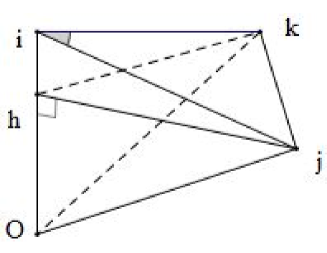
Figure 1: a local triangulation of sphere

Example 1.

Consider the standard sphere $\mathbb{S}^{2}$ imbedded in $\mathds{R}^{3}$. The smooth Gauss curvature of $\mathbb{S}^{2}$ is $+1$ everywhere. Consider a local triangulation of $\mathbb{S}^{2}$ at the north pole, which is denoted as a vertex $i$. $O$ is the origin of $\mathds{R}^{3}$. $h$ is a point lying in $Oi$, see Figure 1. The intersection between the horizonal plane passing through $h$ and $\mathbb{S}^{2}$ is a circle. Divide this circle into $n$ equal portions. Denote any two conjoint points by $j$ and $k$, thus $i$, $j$, $k$ forms a triangle. Denote $x=\angle iOj$. Taking $r_{i}$=$r_{j}$=$r_{k}$=$\overline{ij}/2$=$\sin\frac{x}{2}$, $\Phi_{ij}=\Phi_{ik}=0$ and suitably choosing $\Phi_{jk}$, we can always get a circle packing metric locally with $l_{jk}=2\sin\frac{\pi}{n}\sin x$. Moreover, we can get an infinitesimal triangulation at vertex $i$ by letting $n\rightarrow+\infty$ and $x\rightarrow 0$. By a trivial calculation we can get $\theta_{i}^{jk}=\angle kij=2\arcsin(sin\frac{\pi}{n}cos\frac{x}{2})$, hence the classical discrete Gauss curvature is $K_{i}=2\pi-2n\arcsin(sin\frac{\pi}{n}cos\frac{x}{2})$. It’s obviously that

$$\lim\limits_{n\rightarrow\infty,\,x\rightarrow 0}K_{i}=0.$$

However, the discrete Gauss curvature $R_{i}$ approaches the smooth Gauss curvature in the following way

$$\frac{R_{i}}{\pi}=\frac{K_{i}}{\pi r_{i}^{2}}=\frac{2\pi-2n\arcsin(sin\frac{\pi}{n}cos\frac{x}{2})}{\pi\sin^{2}\frac{x}{2}}\rightarrow+1.$$

$\blacksquare$

Secondly, let’s analyse from the view point of the scaling law of Riemann tensor and Gauss curvature. Recall that, for a $C^{1}$ curve $\gamma:[a,b]\rightarrow M$ in a Riemannian manifold $(M,g)$, the length of the curve is defined to be $L(\gamma,g)=\int_{a}^{b}\sqrt{g(\dot{\gamma}(t),\dot{\gamma}(t))}dt$, where $\dot{\gamma}(t)$ is the tangent vector of $\gamma(t)$ in $M$. So we have $L(\gamma,\tilde{g})=\lambda^{1/2}L(\gamma,g)$ if $\tilde{g}=\lambda g$ for some positive constant $\lambda$. Note that, for a weighted triangulated surface $(M,\mathcal{T},\Phi)$ with circle packing metric $r:V\rightarrow(0,+\infty)$, the length $l_{ij}$ of the edge $\{ij\}$ is given by (1.1). So the quantity corresponding to the Riemannian metric $g$ on the weighted triangulated surface $(M,\mathcal{T},\Phi)$ with circle packing metric $r$ should be quadratic in $r$, among which $r_{i}^{2}$ is the simplest. Furthermore, according to the definition $R_{i}=\frac{K_{i}}{r_{i}^{2}}$, we have $R_{i}(\lambda r_{i}^{2})=\lambda^{-1}R_{i}(r_{i}^{2})$, which has the same form as the transformation for the smooth scalar curvature.

Finally, the Definition 2.1 is geometrically reasonable. Let us recall the original definition of Gauss curvature. We just give a sketch of the definition here and the readers could refer to [S] for details. Suppose $M$ is a surface embedded in $\mathds{R}^{3}$ and $\nu$ is the unit normal vector of $M$ in $\mathds{R}^{3}$. $\nu$ defines the well-known Gauss map $\nu:M\rightarrow S^{2}\subset\mathds{R}^{3}$. Then the Gauss curvature at $p\in M$ is defined as

$$K(p)=\lim_{A\rightarrow p}\frac{Aera~{}\nu(A)}{Aera~{}A},$$

where the limit is taken as the region $A$ around $p$ becomes smaller and smaller. For the weighted triangulated surface $(M,\mathcal{T},\Phi)$ with circle packing metric $r$, assume it is embedded in $\mathds{R}^{3}$ and take the normal vector as a set-valued function, then the definition of discrete Gauss curvature $R_{i}=\frac{K_{i}}{r_{i}^{2}}$ is an approximation of the original Gauss curvature up to a uniform constant $\pi$, as the numerator $K_{i}$ is the measure of the set-valued function $\nu$ and the denominator $r_{i}^{2}$ is the area of the disk with radius $r_{i}$ up to a uniform constant $\pi$.

Note that the classical discrete Gauss curvature satisfies the Gauss-Bonnet identity (1.3). If we define a discrete measure $\mu$ on the vertices by $\mu_{i}=r_{i}^{2}$, then we have

$$\int_{M}fd\mu=\sum_{i=1}^{N}f_{i}r_{i}^{2}$$ (2.1)

for any $f\in C(V)$. Using this discrete measure, we have the following discrete version of Gauss-Bonnet formula

$$\int_{M}Rd\mu=\sum_{i}R_{i}d\mu_{i}=2\pi\chi(M).$$ (2.2)

In this sense, the average curvature is

$$R_{av}=\frac{\int_{M}Rd\mu}{\int_{M}d\mu}=\frac{2\pi\chi(M)}{||r||^{2}},$$ (2.3)

where $||r||^{2}=\sum_{i=1}^{N}r_{i}^{2}$ is the total measure of $M$ with respect to $\mu$.

We give the following table for the corresponding quantities for smooth surfaces and triangulated surfaces.

	Smooth surfaces	Weighted triangulated surfaces
Metric	$g=g_{ij}dx^{i}dx^{j}$	$g_{i}=r_{i}^{2}$
Length	$L(\gamma,g)=\int_{a}^{b}\sqrt{g(\dot{\gamma}(t),\dot{\gamma}(t))}dt$	$l_{ij}=\sqrt{r_{i}^{2}+r_{j}^{2}+2r_{i}r_{j}\cos\Phi_{ij}}$
Measure	$d\mu=\sqrt{\det g_{ij}}dx$	$d\mu_{i}=r_{i}^{2}$
Curvature	Gauss curvature $K$	$R_{i}=\frac{K_{i}}{r_{i}^{2}}$
Total curvature	$\int_{M}Kd\mu=2\pi\chi(M)$	$\sum_{i}R_{i}d\mu_{i}=2\pi\chi(M)$

Table 1: Corresponding between smooth surfaces and triangulated surfaces

For the curvature $R_{i}$ defined by (2.1), it is natural to consider the corresponding combinatorial Yamabe problem, i.e. does there exist any circle packing metric $r$ with constant curvature $R_{i}$ ? Inspired by [CL1, Ge, G1, L1], we study the combinatorial Yamabe problem by the combinatorial curvature flows introduced in the following.

3 The 2-dimensional combinatorial Ricci flow

3.1 Definition of 2-dimensional combinatorial Ricci flow

Ricci flow was introduced by Hamilton [Ham2] to study the low dimension topology. For a closed Riemannian manifold $(M^{n},g_{ij})$, the Ricci flow is defined as

$$\frac{\partial}{\partial t}g_{ij}=-2R_{ij}$$ (3.1)

with normalization

$$\frac{\partial}{\partial t}g_{ij}=\frac{2}{n}rg_{ij}-2R_{ij},$$ (3.2)

where $r$ is the average of the scalar curvature. Ricci flow is a powerful tool and has lots of applications. Specially, it has been used to prove the Poincaré conjecture [P1, P2, P3]. For a closed surface $(M^{2},g_{ij})$, the Ricci flow equation (3.1) is reduced to

$$\frac{\partial}{\partial t}g_{ij}=-Rg_{ij}$$ (3.3)

with the normalization

$$\frac{\partial}{\partial t}g_{ij}=(r-R)g_{ij},$$ (3.4)

where $R$ is the scalar curvature. It is proved [Ham1, CH1] that, for any closed surface with any initial Riemannian metric, the solution of the normalized Ricci flow (3.4) exists for all time and converges to a constant curvature metric conformal to the initial metric as time goes to infinity. It is further pointed out by Chen, Lu and Tian [CLT] that the Ricci flow can be used to give a new proof of the famous uniformization theorem of Riemann surfaces. The discrete version of surface Ricci flow was first introduce by Chow and Luo in [CL1], in which they gave another proof of Thurston’s existence of circle packing theorem. In this subsection, we will introduce a different combinatorial Ricci flow on surfaces to study the constant curvature problem of $R_{i}$.

Definition 3.1.

For a weighted triangulated surface $(M,\mathcal{T},\Phi)$ with circle packing metric $r$, the combinatorial Ricci flow is defined as

$$\frac{dg_{i}}{dt}=-R_{i}g_{i},$$ (3.5)

where $g_{i}=r_{i}^{2}$.

Following Hamilton’s approach, we introduce the following normalization of the flow (3.5)

$$\frac{dg_{i}}{dt}=(R_{av}-R_{i})g_{i},$$ (3.6)

where $R_{av}$ is the average curvature of $R_{i}$ defined by (2.3). It is easy to check that the total measure $\mu(M)=||r||^{2}$ of $M$ with respect to $\mu$ is invariant along the normalized flow (3.6), from which we know that the average curvature $R_{av}=\frac{2\pi\chi(M)}{||r||^{2}}$ is invariant along (3.6). As our goal is to study the existence of constant combinatorial curvature metric, we will focus on the properties of the flow (3.6) in the following. We assume $r(0)\in\mathbb{S}^{N-1}$ and then $r(t)\in\mathbb{S}^{N-1}$ along the flow in the following.

The flows (3.5) and (3.6) differ only by a change of scale in space and a change of parametrization in time. Let $t,r,R$ denote the variables for the unnormalized flow (3.5), and $\tilde{t},\tilde{r},\tilde{R}$ for the normalized flow (3.6). Suppose $r(t)$, $t\in[0,T)$, is a solution of (3.5). Set $\tilde{r}(\tilde{t})=\varphi(t)^{1/2}r(t)$, where $\varphi(t)=||r||^{-2}$ and $\tilde{t}=\int_{0}^{t}\varphi(\tau)d\tau$. Then we have

$$||\tilde{r}||^{2}=1,\ \tilde{R}_{i}=\varphi(t)^{-1}R_{i},\ \tilde{R}_{av}=\varphi(t)^{-1}R_{av}=2\pi\chi(M).$$

This gives

$$\frac{d\tilde{g}_{i}}{d\tilde{t}}=\frac{d\tilde{r}_{i}^{2}}{dt}\frac{dt}{d\tilde{t}}=(\varphi^{\prime}r_{i}^{2}+\varphi\frac{dr_{i}^{2}}{dt})\varphi^{-1}=(\varphi^{\prime}\varphi^{-1}\tilde{r}_{i}^{2}-\varphi R_{i}r_{i}^{2})\varphi^{-1}=(\tilde{R}_{av}-\tilde{R}_{i})\tilde{g}_{i},$$

where, in the last step, we use

$$\varphi^{\prime}=\frac{d}{dt}||r||^{-2}=-||r||^{-4}\frac{d}{dt}||r||^{2}=2\pi\chi(M)\varphi^{2}.$$

Conversely, if $\tilde{r}(\tilde{t}),\tilde{t}\in[0,\tilde{T})$, is a solution of (3.6), set $r(t)=\varphi(\tilde{t})^{1/2}\tilde{r}(\tilde{t})$, where

$$\varphi(\tilde{t})=e^{-\tilde{R}_{av}\tilde{t}},\ t=\int_{0}^{\tilde{t}}\varphi(\tau)d\tau.$$

Then it is easy to check that $\frac{dg_{i}}{dt}=-R_{i}g_{i}$.

For simplicity, we will set $u_{i}=\ln g_{i}$ in the following. Then the flows (3.5) and (3.6) could be written as

$$\dot{u}=-R$$ (3.7)

and

$$\dot{u}=R_{av}\textbf{1}-R$$ (3.8)

respectively, where $u=(u_{1},\cdots,u_{N})^{T}$, $\textbf{1}=(1,\cdots,1)^{T}$ and $R=(R_{1},\cdots,R_{N})^{T}$.

3.2 Discrete Laplace operator

Since $\mu$ is an analogy of the area element, we can define an inner product $\langle\cdot,\cdot\rangle$ on $(M,\mathcal{T},\Phi)$ with circle packing metric $r$ by

$$\langle f,h\rangle=\sum_{i=1}^{N}f_{i}h_{i}r_{i}^{2}=h^{T}\Sigma f$$ (3.9)

for any real functions $f,h\in C(V)$, where

$$\Sigma\triangleq diag\{r_{1}^{2},\cdots,r_{N}^{2}\}.$$

A combinatorial operator $S:C(V)\rightarrow C(V)$ is said to be self-adjoint if

$$\langle Sf,h\rangle=\langle f,Sh\rangle$$

for any $f,h\in C(V)$.

The classical discrete Laplace operator [CHU] $``\Delta"$ is often written in the following form

$$\Delta f_{i}=\sum_{i\sim j}\omega_{ij}(f_{j}-f_{i}),$$

where the weight $\omega_{ij}$ can be arbitrarily selected for different purpose. Bennett Chow and Feng Luo [CL1] first gave a special weight which comes from the dual structure of circle patterns, while Glickenstein [G1] gave a similar weight in three dimension. The curvature $K_{i}$ is determined by the circle packing metric $r$. Consider the curvature as a function of $u$, where $u_{i}=\ln g_{i}=2\ln r_{i}$ are coordinate transformations, then Bennett Chow and Feng Luo’s discrete Laplacian $\Delta_{CL}$ can be interpreted [Ge] as the Jacobian of curvature map, i.e. $\Delta_{CL}=-2L$, where

$$L=\frac{\partial(K_{1},\cdots,K_{N})}{\partial(u_{1},\cdots,u_{N})}.$$ (3.10)

It is noticeable that symbol $L$ above is different from that in [Ge] by a factor 2, which comes from the coordinate transformations.

Using the discrete measure $\mu_{i}=r_{i}^{2}$, we can give a new definition of discrete Laplace operator, which is slightly different from that in [CL1, Ge].

Definition 3.2.

For a weighted triangulated surface $(M,\mathcal{T},\Phi)$ with circle packing metric $r:V\rightarrow(0,+\infty)$, the discrete Laplace operator $\Delta:C(V)\rightarrow C(V)$ is defined as

$$\Delta f_{i}=\frac{1}{r_{i}^{2}}\sum_{j\sim i}(-\frac{\partial K_{i}}{\partial u_{j}})(f_{j}-f_{i})$$ (3.11)

for $f\in C(V)$.

The following property of $L$ will be used frequently in the rest of the paper.

Lemma 3.3.

([CL1], Proposition 3.9.) $L$ is positive semi-definite with rank $N$-$1$ and kernel $\{t\textbf{1}|t\in\mathds{R}\}$. Moreover, $\frac{\partial K_{i}}{\partial u_{i}}>0$, $\frac{\partial K_{i}}{\partial u_{j}}<0$ for $i\sim j$ and $\frac{\partial K_{i}}{\partial u_{j}}=0$ for others.

Using this lemma, we can write discrete Laplace operator as a matrix, that is,

$$\Delta=-\Sigma^{-1}L$$

with

$$\Delta f=-\Sigma^{-1}Lf.$$

Note that the term $-\frac{\partial K_{i}}{\partial u_{j}}>0$ for $i\sim j$ in the definition of the operator $\Delta$, thus it could be taken as a weight on the edges. We sometimes denote this weight as $w_{ij}$ in the following if there is no confusion. This implies that $\Delta$ is a standard Laplacian operator defined on the weighted triangulated surface $(M,\mathcal{T},\Phi)$ with circle packing metric $r$ and measure $\mu$. And it is easy to get

$$\langle\Delta f,g\rangle=g^{T}\Sigma(-\Sigma^{-1}Lf)=-g^{T}Lf=\langle f,\Delta g\rangle.$$

Hence the Laplacian operator $\Delta$ is self-adjoint with respect to $\langle\cdot,\cdot\rangle$. Moreover, if we define

$$|\nabla f|_{i}^{2}=\frac{1}{2r_{i}^{2}}\sum_{j\thicksim i}(-L_{ij})(f_{j}-f_{i})^{2},$$

then we can derive

$$\langle|\nabla f|^{2},\textbf{1}\rangle=\sum_{i=1}^{N}|\nabla f|_{i}^{2}r_{i}^{2}=\sum_{j\thicksim i}(-L_{ij})(f_{j}-f_{i})^{2}=f^{T}Lf=-\langle f,\Delta f\rangle.$$ (3.12)

Using the discrete measure $\mu$ introduced in (2.1), (3.12) can be written in an integral form

$$\int_{M}|\nabla f|^{2}d\mu=-\int_{M}f\Delta fd\mu.$$

When the circle packing metric evolves along the flow (3.6), so is the curvature $R_{i}$. The evolution of $R_{i}$ is very simple and it has almost the same form as the evolution of scalar curvature along the Ricci flow on surfaces derived by Hamilton in [Ham1].

Lemma 3.4.

Along the normalized combinatorial Ricci flow (3.6), the curvature $R_{i}$ satisfies the evolution equation

$$\frac{dR_{i}}{dt}=\Delta R_{i}+R_{i}(R_{i}-R_{av}).$$ (3.13)

Proof. As $u_{i}=\ln r_{i}^{2}$, we have $\frac{\partial}{\partial u_{j}}=\frac{1}{2}r_{j}\frac{\partial}{\partial r_{j}}$. Then we have

$$\frac{dR_{i}}{dt} =\sum_{j}\frac{\partial R_{i}}{\partial u_{j}}\frac{du_{j}}{dt}$$

$$=\sum_{j}(\frac{1}{r_{i}^{2}}\frac{\partial K_{i}}{\partial u_{j}}-\frac{K_{i}}{r_{i}^{4}}r_{i}r_{j}\delta_{ij})(R_{av}-R_{j})$$

$$=\frac{1}{r_{i}^{2}}\sum_{j}\frac{\partial K_{i}}{\partial u_{j}}(R_{av}-R_{j})-R_{i}(R_{av}-R_{i})$$

$$=-\frac{1}{r_{i}^{2}}\sum_{j}\frac{\partial K_{i}}{\partial u_{j}}R_{j}+R_{i}(R_{i}-R_{av})$$

$$=\frac{1}{r_{i}^{2}}\sum_{j\sim i}(-\frac{\partial K_{i}}{\partial u_{j}})(R_{j}-R_{i})+R_{i}(R_{i}-R_{av}).$$

In the last two steps, Lemma 3.3 is used. $\blacksquare$

Thus the evolution equation (3.13) of $R_{i}$ is a reaction-diffusion equation. In fact, suppose $\Omega$ is a subset of $V$, set $\nabla_{ij}f=f_{j}-f_{i}$ for $f\in C(V)$ and $i\sim j$, and denote

$$\partial\Omega=\{\{ij\}\in E|i\in\Omega,j\in\Omega^{c}\},$$

then it is easy to check that

$$\frac{d}{dt}\int_{\Omega}Rd\mu=\sum_{i\in\Omega,j\in\Omega^{c},i\sim j}(-\frac{\partial K_{i}}{\partial u_{j}})(R_{j}-R_{i})=\int_{\partial\Omega}\nabla Rdw.$$

Then we have similar explanation as the smooth Ricci flow for equation (3.6).

3.3 Maximum principle

As the evolution equation (3.13) is a heat-type equation, we have the following discrete maximum principle for such equations. Such maximum principle is almost standard, for completeness, we write it down here.

Theorem 3.5.

(Maximum Principle) Let $f:V\times[0,T)\rightarrow\mathds{R}$ be a $C^{1}$ function such that

$$\frac{\partial f_{i}}{\partial t}\geq\Delta f_{i}+\Phi_{i}(f_{i}),\ \ \forall(i,t)\in V\times[0,T)$$

where $\Phi_{i}:\mathds{R}\rightarrow\mathds{R}$ is a local Lipschitz function. Suppose there exists $C_{1}\in\mathds{R}$ such that $f_{i}(0)\geq C_{1}$ for all $i\in V$. Let $\varphi$ be the solution to the associated ODE

$$\left\{\begin{array}[]{ll}\frac{d\varphi}{dt}=\Phi_{i}(\varphi)\\ \varphi(0)=C_{1},\end{array}\right.$$

then

$$f_{i}(t)\geq\varphi(t)$$

for all $(i,t)\in V\times[0,T)$ such that $\varphi(t)$ exists.

Similarly, suppose $f:V\times[0,T)\rightarrow\mathds{R}$ be a $C^{1}$ function such that

$$\frac{\partial f_{i}}{\partial t}\leq\Delta f_{i}+\Phi_{i}(f_{i}),\ \ \forall(i,t)\in V\times[0,T).$$

Suppose there exists $C_{2}\in\mathds{R}$ such that $f_{i}(0)\leq C_{2}$ for all $i\in V$. Let $\psi$ be the solution to the associated ODE

$$\left\{\begin{array}[]{ll}\frac{d\psi}{dt}=\Phi_{i}(\psi)\\ \psi(0)=C_{2},\end{array}\right.$$

then

$$f_{i}(t)\leq\psi(t)$$

for all $(i,t)\in V\times[0,T)$ such that $\psi(t)$ exists.

Remark 3.

In fact, Theorem 3.5 is valid for general Laplacian operators defined as

$$\Delta f_{i}=\sum_{j\sim i}a_{ij}(t)(f_{j}-f_{i}),$$

where $a_{ij}\geq 0$, but not required to satisfy the symmetry condition $a_{ij}=a_{ji}$.

The proof of Theorem 3.5 is almost the same as that in [CK], we give a proof of it here just for completeness.

Proposition 3.6.

Let $f:V\times[0,T)\rightarrow\mathds{R}^{N}$ be a $C^{1}$ solution to the heat equation

$$\frac{\partial f}{\partial t}=\Delta f,$$

i.e.

$$\frac{\partial f_{i}}{\partial t}=\Delta f_{i}=\sum_{j\sim i}a_{ij}(t)(f_{j}-f_{i}).$$

If there are constants $C_{1}\leq C_{2}\in\mathds{R}$ such that $C_{1}\leq f_{i}(0)\leq C_{2}$ for all $i\in V$, then

$$C_{1}\leq f_{i}(t)\leq C_{2},\ \ \ \forall(i,t)\in V\times[0,T).$$

This proposition follows from the following more general theorem.

Theorem 3.7.

Suppose $f:V\times[0,T)\rightarrow\mathds{R}^{N}$ be a $C^{1}$ function with $f_{i}(0)\geq\alpha$ for some constant $\alpha\in\mathds{R}$, and $f$ satisfies

$$\frac{\partial f_{i}}{\partial t}\geq\Delta f_{i}$$

at any $(i,t)\in V\times[0,T)$ such that $f_{i}(t)<\alpha$. Then

$$f_{i}(t)\geq\alpha$$

for all $(i,t)\in V\times[0,T)$.

Proof. Note that if $H:V\times[0,T)\rightarrow\mathds{R}$ is a $C^{1}$ function and $(i,t_{0})$ is the vertex and time where $H_{i}(t)$ attains its minimum among all vertices and earlier times, namely

$$H_{i}(t_{0})=\min_{(j,t)\in V\times[0,t_{0}]}H_{j}(t),$$

then

$$\frac{\partial H_{i}}{\partial t}(t_{0})\leq 0,\Delta H_{i}(t_{0})\geq 0.$$

Consider a function $H$ defined by $H_{i}(t)=\left(f_{i}(t)-\alpha\right)+\varepsilon t+\varepsilon,$ where $\varepsilon$ is any positive constant. Then $H_{i}(0)\geq\varepsilon>0$, and

$$\frac{\partial H_{i}}{\partial t}=\frac{\partial f_{i}}{\partial t}+\varepsilon\geq\Delta f_{i}+\varepsilon=\Delta H_{i}+\varepsilon$$

for $(i,t)\in V\times[0,T)$ satisfies $f_{i}(t)\leq\alpha$. Thus we just need to prove that $H_{i}(t)>0$ for $(i,t)\in V\times[0,T)$.

Suppose that $(i,t_{0})$ is the first point in $V\times[0,T)$ such that $H_{i}(t_{0})=0$. Then

$$f_{i}(t_{0})=H_{i}(t_{0})+\alpha-\varepsilon t_{0}-\varepsilon=\alpha-\varepsilon t_{0}-\varepsilon<\alpha.$$

Then we have

$$0\geq\frac{\partial H_{i}}{\partial t}(t_{0})\geq\Delta H_{i}(t_{0})+\varepsilon\geq\varepsilon>0,$$

which is a contradiction. And the theorem follows from $\varepsilon\rightarrow 0$. $\blacksquare$

Now suppose $\beta:V\times[0,T)\rightarrow\mathds{R}$ be a function.

Proposition 3.8.

Let $f:V\times[0,T)\rightarrow\mathds{R}$ be a $C^{1}$ function such that

$$\frac{\partial f_{i}}{\partial t}\geq\Delta f_{i}+\beta_{i}f_{i}.$$

And for each $\tau\in[0,T)$, $\exists C_{\tau}<\infty$ such that $\beta_{i}(t)<C_{\tau}$ for $(i,t)\in V\times[0,\tau]$. If $f_{i}\geq 0$ for all $i\in V$, then $f_{i}(t)\geq 0$ for all $(i,t)\in V\times[0,T)$.

Proof. Given $\tau\in(0,T)$, define

$$J_{i}(t)=e^{-C_{\tau}t}f_{i}(t),$$

then

$$\frac{\partial J_{i}}{\partial t}\geq\Delta J_{i}+(\beta_{i}-C_{\tau})J_{i}.$$

Since $\beta_{i}(t)\leq C_{\tau}$ for all $(i,t)\in V\times[0,\tau]$, then we have

$$\frac{\partial J_{i}}{\partial t}\geq\Delta J_{i}$$

for $(i,t)\in V\times[0,\tau]$ such that $J_{i}(t)<0$. Then by the Theorem 3.7, we have $J_{i}(t)\geq 0$, and then $f_{i}(t)\geq 0$ for any $(i,t)\in V\times[0,T)$. $\blacksquare$

Now we give the proof of Theorem 3.5.

Proof of Theorem 3.5: We take the lower bound to prove, and proof for the upper bound is similar. By assumption, we have

$$\frac{\partial}{\partial t}(f_{i}-\varphi)\geq\Delta(f_{i}-\varphi)+\Phi_{i}(f_{i})-\Phi_{i}(\varphi).$$

The assumptions on the initial data imply that

$$(f_{i}-\varphi)(0)\geq 0,\forall i\in V.$$

Let $\tau\in(0,T)$, then $\exists C_{\tau}<\infty$ such that $|f_{i}(t)|<C_{\tau}$ for all $(i,t)\in V\times[0,\tau]$ and $|\varphi(t)|<C_{\tau}$ for $t\in[0,\tau]$. Since $F$ is locally Lipschitz, then we have

$$|\Phi_{i}(f_{i})-\Phi_{i}(\varphi)|\leq L_{\tau}|f_{i}-\varphi|,\forall i\in V$$

for some positive constant $L_{\tau}>0$. Then

$$\frac{\partial}{\partial t}(f_{i}-\varphi)\geq\Delta(f_{i}-\varphi)-L_{\tau}Sgn(f_{i}-\varphi)\cdot(f_{i}-\varphi),\forall(i,t)\in V\times[0,\tau].$$

Applying Proposition 3.8, we get

$$f_{i}(t)-\varphi(t)\geq 0,\forall(i,t)\in V\times[0,\tau].$$

And the theorem follows from $\tau\in[0,T)$ is arbitrary. $\blacksquare$

Applying Theorem 3.5 to (3.13) with vanishing initial value, we can easily get the following corollary.

Corollary 3.9.

If $R_{i}(0)\geq 0$ ($R_{i}(0)\leq 0$) for all $i\in V$, then $R_{i}(t)\geq 0$ ($R_{i}(t)\leq 0$) for all $i\in V$ as long as the flow exists, i.e. the positive and negative curvatures are preserved along the normalized flow (3.6).

Set $R_{max}(t)=\max_{i\in V}R_{i}(t)$ and $R_{min}(t)=\min_{i\in V}R_{i}(t)$. Applying Theorem 3.5 to (3.13) with general initial data, we get the following lower bounds for $R_{i}(t)$. For simplicity, We just state it in the form parallel to that given in [CK].

Lemma 3.10.

(Lower Bound) Let $r_{i}(t)$ be a solution to the normalized combinatorial Ricci flow (3.13) on a closed triangulated surface $(M,T,\Phi)$.

• If $\chi(M)<0$, then

  $$R_{i}-R_{av}\geq\frac{R_{av}}{1-(1-\frac{R_{av}}{R_{min}(0)})e^{R_{av}t}}-R_{av}\geq(R_{min}(0)-R_{av})e^{R_{av}t}.$$

• If $\chi(M)=0$, then

  $$R_{i}\geq\frac{R_{min}(0)}{1-R_{min}(0)t}>-\frac{1}{t}.$$

• If $\chi(M)>0$ and $R_{min}(0)<0$, then

  $$R\geq\frac{R_{av}}{1-(1-\frac{R_{av}}{R_{min}(0)})e^{R_{av}t}}\geq R_{min}(0)e^{-R_{av}t}.$$

Notice that in each case, the right hand side of the lower bound estimate tends to 0 as $t\rightarrow\infty$. However, for the upper bound, the situation is not so good. The solution of the ODE

$$\left\{\begin{array}[]{ll}\frac{ds}{dt}&=s(s-R_{av})\\ s(0)&=s_{0}\end{array}\right.$$

corresponding to (3.13) is

$$\begin{aligned} s(t)=\left\{\begin{array}[]{ll}0,&\hbox{$s_{0}=0$}\\ \frac{s_{0}}{1-s_{0}t},&\hbox{$s_{0}\neq 0,\ \chi(M)=0$}\\ \frac{R_{av}}{1-(1-\frac{R_{av}}{s_{0}})e^{R_{av}t}},&\hbox{$s_{0}\neq 0,\ \chi(M)\neq 0$}\end{array}\right.\end{aligned}.$$

If $s_{0}>\max\{R_{av},0\}$, there is $T<\infty$ given by

$$T=\left\{\begin{array}[]{ll}-\frac{1}{R_{av}}\ln\left(1-\frac{R_{av}}{s_{0}}\right)>0,&\hbox{$\chi(M)\neq 0$}\\ \frac{1}{s_{0}},&\hbox{$\chi(M)=0$}\end{array}\right.$$

such that

$$\lim_{t\rightarrow T^{-}}s(t)=+\infty.$$

The implies that, in the case of $R_{max}(0)>\max\{R_{av},0\}$, Theorem 3.5 will not give us good upper bounds for the curvature along the combinatorial Ricci flow (3.13). However, in the case of $R_{max}(0)<0$, we have good upper bounds.

Lemma 3.11.

If $R_{i}(0)<0$ for all $i\in V$, then we have

$$R_{i}(t)-R_{av}\leq R_{av}\left(1-\frac{R_{av}}{R_{max}(0)}\right)e^{R_{av}t}.$$

These results are almost parallel to that of the smooth Ricci flow on surfaces.

3.4 Convergence of the 2-dimensional combinatorial Ricci flow

Combining Lemma (3.10) with (3.11) gives

Theorem 3.12.

Suppose $(M,\mathcal{T},\Phi)$ is a weighted triangulated surface with initial circle packing metric $r(0)$ satisfying $R_{i}(0)<0$ for all $i\in V$, then there exists a negative constant curvature metric $r^{*}$ on $(M,\mathcal{T},\Phi)$. Furthermore, the solution $r(t)$ to the normalized combinatorial Ricci flow (3.6) exists for all time and converges exponentially fast to $r^{*}$ as $t\rightarrow+\infty$.

Theorem 3.12, derived by combinatorial maximum principle, implies more than it seems. It claims that, if there is a metric with all curvatures negative, then there always exists a negative constant curvature metric, and vice versa. Using this fact, we will give a combinatorial and topological condition which is equivalent to the existence of negative constant curvature metric in subsection 3.6. For the convergence of combinatorial Ricci flow, the negative initial curvature condition in Theorem 3.12 is a little restrictive. It is natural to consider Hamilton’s approach to generalize this result. However, we found that there is some technical difficulties to go further with Hamilton’s approach in this case. By studying critical points of (3.6), which is an ODE system, we can get the following local convergence result.

Theorem 3.13.

Suppose $r^{*}$ is a constant $R$-curvature metric on a weighted triangulated surface $(M,\mathcal{T},\Phi)$. If the first positive eigenvalue $\lambda_{1}$ of $-\Delta$ at $r^{*}$ satisfies

$$\lambda_{1}(-\Delta)>R_{av}^{*}=\frac{2\pi\chi(M)}{||r^{*}||^{2}}$$ (3.14)

and $||r(0)-r^{*}||^{2}$ is small enough, then the solution to the normalized combinatorial Ricci flow (3.6) exists for $t\in[0,+\infty)$ and converges exponentially fast to $r^{*}$.

Proof. We can rewrite the normalized combinatorial Ricci flow (3.6) as

$$\frac{dr_{i}}{dt}=\frac{1}{2}(R_{av}-R_{i})r_{i}.$$

Set $\Gamma_{i}(r)=\frac{1}{2}(R_{av}-R_{i})r_{i}$, then the Jacobian matrix of $\Gamma(r)$ is given by

$$(D_{r}\Gamma(r))_{ij}=\frac{\partial}{\partial r_{j}}\left(\frac{1}{2}(R_{av}-R_{i})r_{i}\right)=\frac{1}{2}(R_{av}-R_{i})\delta_{ij}+(R_{i}\delta_{ij}-R_{av}\frac{r_{i}r_{j}}{||r||^{2}})-\frac{1}{r_{i}r_{j}}\frac{\partial K_{i}}{\partial u_{j}}.$$

Denote $\Lambda=\Sigma^{-\frac{1}{2}}L\Sigma^{-\frac{1}{2}}$, then $\Lambda\sim\Sigma^{-\frac{1}{2}}\Lambda\Sigma^{\frac{1}{2}}=-\Delta$, hence $\lambda_{1}(-\Delta)=\lambda_{1}(\Lambda)$. At the constant curvature metric point $r^{*}$, we have

$$D_{r}\Gamma|_{r^{*}}=R_{av}\left(I-\frac{rr^{T}}{||r||^{2}}\right)-\Sigma^{-\frac{1}{2}}L\Sigma^{-\frac{1}{2}}=R_{av}\left(I-\frac{rr^{T}}{||r||^{2}}\right)-\Lambda.$$

Select an orthonormal matrix $P$ such that

$$P^{T}\Lambda P=diag\{0,\lambda_{1}(\Lambda),\cdots,\lambda_{N-1}(\Lambda)\}.$$

Suppose $P=(e_{0},e_{1},\cdots,e_{N-1})$, where $e_{i}$ is the $(i+1)$-column of $P$. Then $\Lambda e_{0}=0$ and $\Lambda e_{i}=\lambda_{i}e_{i},\,1\leq i\leq N-1$, which implies $e_{0}=r/\|r\|$ and $r\perp e_{i},\,1\leq i\leq N-1$. Hence $\big{(}I_{N}-\frac{rr^{T}}{\|r\|^{2}}\big{)}e_{0}=0$ and $\big{(}I_{N}-\frac{rr^{T}}{\|r\|^{2}}\big{)}e_{i}=e_{i}$, $1\leq i\leq N-1$, which implies $P^{T}\big{(}I_{N}-\frac{rr^{T}}{\|r\|^{2}}\big{)}P=diag\{0,1,\cdots,1\}$. Therefore,

$$D_{r}\Gamma\big{|}_{r^{*}}=P\cdot diag\{0,R_{av}-\lambda_{1}(\Lambda),\cdots,R_{av}-\lambda_{N-1}(\Lambda)\}\cdot P^{T}.$$

If $\lambda_{1}(\Lambda)>R_{av}^{*}=\frac{2\pi\chi(M)}{||r^{*}||^{2}}$, then $D_{r}\Gamma\big{|}_{r^{*}}$ is negative semi-definite with kernel $\{cr|c\in\mathbb{R}\}$ and $rank\,(D_{r}\Gamma\big{|}_{r^{*}})=N-1$. Note that, along the flow (3.6), $||r||^{2}$ is invariant. Thus the kernel is transversal to the flow. This implies that $D_{r}\Gamma|_{r^{*}}$ is negative definite on $\mathbb{S}^{N-1}$ and $r^{*}$ is a local attractor of the normalized combinatorial Ricci flow (3.6). Then the conclusion follows from the Lyapunov Stability Theorem([P], Chapter 5). $\blacksquare$

If $\chi(M)\leq 0$, we always have $\lambda_{1}(-\Delta)>0\geq R_{av}^{*}=\frac{2\pi\chi(M)}{||r^{*}||^{2}}$, thus we get

Corollary 3.14.

Suppose there is a nonpositive constant curvature metric $r^{*}$ on a weighted triangulated surface $(M,\mathcal{T},\Phi)$ with $\chi(M)\leq 0$. If $||r(0)-r^{*}||^{2}$ is small enough, then the solution to the normalized combinatorial Ricci flow (3.6) exists for $t\in[0,+\infty)$ and converges exponentially fast to $r^{*}$.

Before proving the global results, we first check that the convergence of the flow (3.6) ensures the existence of the constant curvature metric. More generally, we have the following result.

Lemma 3.15.

Suppose that the solution to the flow (3.6) lies in a compact region in $\mathds{R}^{N}_{>0}$, then there exists a constant curvature metric $r^{*}$. Moreover, there exists a sequence of metrics which converge to $r^{*}$ along this flow.

Proof. Consider the Ricci potential

$$F(u)=\int_{u_{0}}^{u}\sum_{i=1}^{N}(K_{i}-R_{av}r_{i}^{2})du_{i},$$

where $u_{i}=\ln r_{i}^{2}$ and $u_{0}\in\mathds{R}^{N}$ is an arbitrary point. If we set $\varphi_{i}=K_{i}-\frac{2\pi\chi(M)}{||r||^{2}}r_{i}^{2}$, by direct calculations, we have

$$\frac{\partial\varphi_{i}}{\partial u_{j}}=\frac{\partial\varphi_{j}}{\partial u_{i}}.$$

As the domain of $u$ is simply connected, this implies that the integration is path independent and then the Ricci potential is well defined. Suppose $t\in[0,T)$ and $T$ is the maximal existing time of $u(t)$. Then $\{u(t)\}\subset\subset\mathds{R}^{N}$ implies $T=+\infty$, otherwise $u(t)$ will run out of the compact region. $\{u(t)\}\subset\subset\mathds{R}^{N}$ also implies that $F(u(t))$ is bounded. Moreover,

$$\frac{d}{dt}F(u(t))=(\nabla_{u}F)^{T}\cdot\dot{u}=-\sum\left(\frac{K_{i}}{r_{i}}-\frac{2\pi\chi(M)}{||r||^{2}}r_{i}\right)^{2}=-\sum_{i}(R_{i}-R_{av})^{2}r_{i}^{2}\leq 0.$$

Hence $\lim_{t\rightarrow+\infty}F(u(t))$ exists. Then by the mean value theorem, there exists a sequence $\xi_{n}\in(n,n+1)$ such that

$$F(u(n+1))-F(u(n))=(F(u(t)))^{\prime}|_{t=\xi_{n}}=-\sum_{i}(R_{i}-R_{av})^{2}r_{i}^{2}(\xi_{n})\rightarrow 0$$

as $n\rightarrow+\infty$. Since $\{r(t)\}\subset\subset R_{>0}^{N}$, we can further select a subsequence $t_{k}=\xi_{n_{k}}$ such that $r(t_{k})\rightarrow r^{*}$ as $k\rightarrow+\infty$. Combining $\sum_{i}r_{i}^{2}(R_{i}-R_{av})^{2}(\xi_{n_{k}})\rightarrow 0$, we know that $r^{*}$ determines a constant $R$-curvature. $\blacksquare$

Corollary 3.16.

Suppose that the solution to flow (3.6) exists for all time and converges to $r(+\infty)$, then $r(+\infty)$ is a constant curvature metric.

Remark 4.

For the Ricci potential functional $F$ used in the proof of Lemma 3.15, the primitive form of this type of functional was first constructed by Colin de Verdière in [DV] and then further studied by Chow and Luo in [CL1]. Our definition is a modification of their constructions.

For the Ricci potential $F$ introduced in the proof of Lemma 3.15, we further have the following property.

Lemma 3.17.

Given a weighted triangulated surface $(M,\mathcal{T},\Phi)$. Assume there is a constant curvature circle packing metric $r^{*}$ on $(M,\mathcal{T},\Phi)$. Define the Ricci potential as

$$F(u)=\int_{u^{*}}^{u}\sum_{i=1}^{N}(K_{i}-R_{av}r_{i}^{2})du_{i}.$$ (3.15)

Denote

$$\mathscr{U}_{a}\triangleq\{u\in\mathds{R}^{N}|\sum_{i}u_{i}=a\},\ \ \ a\in\mathds{R}.$$

If $\lambda_{1}(-\Delta)>R_{av}$ for all $r\in\mathds{R}_{>0}^{N}$, then

• $Hess_{u}F$ is positive semi-definite with rank $N-1$ and kernel $\{t\mathbf{1}|t\in\mathds{R}\}$.

• Restricted to $\mathscr{U}_{a}$, $F|_{\mathscr{U}_{a}}$ is strictly convex and proper. $F|_{\mathscr{U}_{a}}$ has a unique zero point which is also the unique minimum point. Moreover, $\lim\limits_{u\in\mathscr{U}_{a},\,u\rightarrow\infty}F(u)=+\infty$.

Proof. By direct calculations, we have

$$Hess_{u}F=L-R_{av}\Sigma^{\frac{1}{2}}\left(I-\frac{rr^{T}}{||r||^{2}}\right)\Sigma^{\frac{1}{2}}=\Sigma^{\frac{1}{2}}\left(\Lambda-R_{av}\left(I-\frac{rr^{T}}{||r||^{2}}\right)\right)\Sigma^{\frac{1}{2}}.$$ (3.16)

By the same analysis as that of Theorem 3.13, we know that, if $\lambda_{1}(-\Delta)>R_{av}$, $Hess_{u}F$ is positive semi-definite with $rank(Hess_{u}F)=N-1$ and $Ker(Hess_{u}F)=\{t\mathbf{1}|t\in\mathds{R}\}$.

For the second part of the proof, we follow that of Colin de Verdière [DV] and Chow and Luo[CL1]. It’s easy to see $F(u)=F(u+t\textbf{1})$ for any $t\in\mathds{R}$ and $u\in\mathds{R}^{N}$. As $F$ is invariant along the direction 1, we just need to prove it on $\mathscr{U}_{0}=\{u\in\mathds{R}^{N}|\sum u_{i}=0\}$. A rigorous proof is formulated in Theorem B.2 of [Ge]. In addition, $u^{*}+\frac{a-\textbf{1}^{T}u^{*}}{N}\textbf{1}$ is the unique zero point and minimum point of $F|_{\mathscr{U}_{a}}$. $\blacksquare$

Theorem 3.18.

Suppose $(M,\mathcal{T},\Phi)$ is a weighted triangulated surface and $\lambda_{1}(-\Delta)>R_{av}$ for all $r\in\mathds{R}_{>0}^{N}$. Then the solution to the flow (3.6) converges if and only if there exists a constant curvature metric $r^{*}$. Furthermore, if the solution converges, it converges exponentially fast to the metric of constant curvature.

Proof. The necessary part can be seen from Corollary 3.16. For the sufficient part, without loss of generality, we may assume $r^{*}\in\mathbb{S}^{N-1}$. Consider the flow (3.6) with initial metric $r(0)\in\mathbb{S}^{N-1}\cap\mathds{R}^{N}_{>0}$. Then $r(t)\in\mathbb{S}^{N-1}\cap\mathds{R}^{N}_{>0}$ and $u(t)\in\mathscr{V}_{1}^{*}\triangleq\{u\in\mathds{R}^{N}|\sum_{i}e^{u_{i}}=1\}$ for all $t$. Let $\Pi$ be the orthogonal projection from $\mathscr{V}_{1}^{*}$ to the plane $\mathscr{U}_{0}=\{u\in\mathds{R}^{N}|\sum_{i}u_{i}=0\}$. Then $F(u)=F(\Pi(u))$ and $\Pi(u)\rightarrow\infty$ as $u\rightarrow\infty$. In fact, for a sequence $\{u^{(n)}\}$, $\Pi(u^{(n)})$ is unbounded if and only if $|\Pi(u^{(n)})_{i}-\Pi(u^{(n)})_{j}|=|u^{(n)}_{i}-u^{(n)}_{j}|$ is unbounded. Then Lemma 3.17 implies

$$\lim\limits_{u\rightarrow\infty,\,u\in\mathscr{V}_{1}^{*}}F(u)=+\infty,$$ (3.17)

which means that $F(u)$ is still proper on $\mathscr{V}_{1}^{*}$. Since $F(u(t))^{\prime}\leq 0$, $u(t)$ lies in a compact region in $\mathscr{V}_{1}^{*}$. By Lemma 3.15, the solution exists for $t\in[0,+\infty)$ and there exists a sequence of metrics $r(t_{k})$ which converge to $r^{*}$ as $t_{k}\uparrow+\infty$. Hence $F(u(+\infty))=\lim\limits_{k\rightarrow+\infty}F(u(t_{k}))=F(u^{*})=0$. While Lemma 3.17 says that $u^{*}$ is the unique zero and minimum point of $F$, thus we get $u(t)$ converges to $u^{*}$ as $t\rightarrow+\infty$. The exponentially convergent rate comes from Theorem 3.13. $\blacksquare$

Corollary 3.19.

Suppose $(M,\mathcal{T},\Phi)$ is a weighted triangulated surface with $\chi(M)\leq 0$. Then the solution to the flow (3.6) converges if and only if there exists a constant $R$-curvature metric $r^{*}$. Furthermore, if the solution converges, it converges exponentially fast to the metric of constant curvature.

We expect Corollary 3.19 to be still valid for surfaces with $\chi(M)>0$. However, things are not so satisfactory for general triangulations. In fact, things may become very different and complicated. Assume there exists a constant curvature metric $r^{*}$, we may compare the Ricci potential (3.15) with

$$G(u)=\int_{u^{*}}^{u}\sum_{i=1}^{N}(K_{i}-K_{i}^{*})du_{i},$$

where $K_{i}^{*}=\frac{2\pi\chi(M)}{\|r^{*}\|^{2}}r_{i}^{*2}$, then

$$F(u)-G(u) =\int_{u_{*}}^{u}\sum_{i=1}^{N}(K_{i}^{*}-R_{av}r_{i}^{2})du_{i}$$

$$=2\pi\chi(M)\left(\cfrac{\sum_{i=1}^{N}r_{i}^{*2}(u_{i}-u_{i}^{*})}{\|r^{*}\|^{2}}-\int_{u_{*}}^{u}\cfrac{e^{u_{1}}du_{1}+\cdots+e^{u_{N}}du_{N}}{e^{u_{1}}+\cdots+e^{u_{N}}}\right)$$

$$=2\pi\chi(M)\cfrac{\sum_{i=1}^{N}r_{i}^{*2}(u_{i}-u_{i}^{*})}{\|r^{*}\|^{2}}-2\pi\chi(M)\ln(e^{u_{1}}+\cdots+e^{u_{N}})\bigg{|}_{u^{*}}^{u}.$$

Restricted to the hypersurface $\mathscr{V}^{*}\triangleq\{u\in\mathds{R}^{N}|\sum_{i}e^{u_{i}}=\sum_{i}e^{u_{i}^{*}}\}$, the last term becomes zero, hence

$$F(u)=G(u)+2\pi\chi(M)\cfrac{\sum_{i=1}^{N}r_{i}^{*2}(u_{i}-u_{i}^{*})}{\|r^{*}\|^{2}},\,\,\forall u\in\mathscr{V}^{*}.$$

By similar arguments in the proof of Theorem 3.18, we further have

$$\lim\limits_{u\rightarrow\infty,\,u\in\mathscr{V}^{*}}G(u)=+\infty.$$

One may expect that the growth behavior of $F$ is similar to that of $G$. Unfortunately, there is an obstruction which makes things very complicated. It’s easy to see

$$\lim\limits_{u\rightarrow\infty,\,u\in\mathscr{V}^{*}}\cfrac{\sum_{i=1}^{N}r_{i}^{*2}(u_{i}-u_{i}^{*})}{\|r^{*}\|^{2}}=-\infty.$$

The growth behavior of $F$ is uncertain unless one can compare the growth rates of these two terms concretely. It seems that we can not expect that $G(u)$ succeeds the last term due to the following example.

Example 2.

Given a topological sphere, triangulate it into four faces of a single tetrahedron. Fix weights $\Phi\equiv 0$. Denote $r^{*}=\textbf{1}$, then $r^{*}$ is a constant curvature metric with $R_{i}\equiv\pi$. By direct calculation, we get $Hess_{u}F|_{u^{*}}=(\frac{\sqrt{3}}{6}-\frac{\pi}{4})(4I_{4}-\textbf{1}\textbf{1}^{T})$, which is negative semi-definite with three negative eigenvalues. Up to scaling, $Hess_{u}F$ is negative definite at $r^{*}$. Thus the fixed point $r^{*}=\textbf{1}$ of the ODE system $r_{i}^{\prime}(t)=\frac{1}{2}(R_{av}-R_{i})r_{i}$ (i.e. the flow (3.6)) is a source. For this particular weighted triangulation, the flow (3.6) can never converge to the constant curvature metric $r^{*}$ for any initial value $r(0)$, as $t\rightarrow+\infty$. However, when $t\rightarrow-\infty$, the solution of (3.6) converges to $r^{*}$ if $r(0)\in\mathbb{S}^{N-1}(2)$ is close enough to $r^{*}$.

From the example we know that it is impossible to get an analogous version of Corollary 3.19 when $\chi(M)>0$. However, we can get the following long time existence of (3.6) by maximum principle.

Theorem 3.20.

Given a weighted triangulated surface $(M,\mathcal{T},\Phi)$ with $\chi(M)>0$ and

$$-\sum_{(e,v)\in Lk(I)}(\pi-\Phi(e))+2\pi\chi(F_{I})<0,\ \ \forall I:\,\emptyset\subsetneqq I\subsetneqq V.$$ (3.18)

Suppose $r_{0}$ is a circle packing metric with $R_{i}\geq 0$ for all $i\in V$. Then the solution of (3.6) with initial metric $r_{0}$ exists for all time and lies in a compact region in $\mathds{R}^{N}_{>0}$. Furthermore, there exists $t_{n}\uparrow+\infty$, such that $r(t_{n})$ converges to a constant curvature metric $r^{*}$.

Proof. By Lemma 3.15, we just need to prove that $\{r(t)\}\subset\subset\mathds{R}^{N}_{>0}$. We prove it by contradiction. Suppose

$$\overline{\{r(t)\}}\cap\partial(\mathds{R}^{N}_{>0}\cap\mathbb{S}^{N-1})\neq\emptyset,$$

then there exists a sequence $t_{n}$ such that

$$r(t_{n})\rightarrow r^{*}\in\partial(\mathds{R}^{N}_{>0}\cap\mathbb{S}^{N-1}),$$

where $r^{*}=(0,\cdots,0,r^{*}_{|I|+1},\cdots,r_{N}^{*})$ for some nonempty proper subset $I$ of $V$. By Proposition 4.1 of [CL1], we have

$$\lim_{n\rightarrow+\infty}\sum_{i\in I}K_{i}(r(t_{n}))=-\sum_{(e,v)\in Lk(I)}(\pi-\Phi(e))+2\pi\chi(F_{I})<0.$$ (3.19)

However, by Corollary 3.9, $R_{i}\geq 0$ is preserved along the flow (3.6). Thus $K_{i}\geq 0$ for all $i\in V$, which implies $\lim_{n\rightarrow+\infty}\sum_{i\in I}K_{i}(r(t_{n}))\geq 0$. This contradicts (3.19). $\blacksquare$

Remark 5.

It is easy to see that the triangulation of sphere in Example 2 does not satisfy the condition (3.18).

3.5 The prescribing curvature problem

Using modified combinatorial Ricci flow, we can consider the prescribing curvature problem on a weighted triangulated surface $(M,\mathcal{T},\Phi)$.

Definition 3.21.

Suppose $(M,\mathcal{T},\Phi)$ is a weighted triangulated surface with circle packing metric $r$, $\overline{R}\in C(V)$ is a function defined on $M$. The modified combinatorial Ricci flow with respect to $\overline{R}$ is defined to be

$$\frac{dg_{i}}{dt}=(\overline{R}_{i}-R_{i})g_{i},$$ (3.20)

where $g_{i}=r_{i}^{2}$ as before.

Note that the total measure $\mu(M)=||r||^{2}$ may vary along the modified combinatorial Ricci flow (3.20), which is different from that of (3.6).

$\overline{R}$ is called admissible if there is a circle packing metric $\overline{r}$ with curvature $\overline{R}$. For a given function $\overline{R}\in C(V)$, we can introduce the following modified Ricci potential

$$\overline{F}(u)=\int_{u_{0}}^{u}\sum_{i=1}^{N}\left(K_{i}-\overline{R}_{i}r_{i}^{2}\right)du_{i}.$$ (3.21)

It is easy to check that the modified Ricci potential $\overline{F}$ is well-defined. Furthermore, by direct calculations, we have

$$Hess_{u}\overline{F}=L-\Sigma^{\frac{1}{2}}\left(\begin{array}[]{ccc}\overline{R}_{1}&&\\ &\ddots&\\ &&\overline{R}_{N}\\ \end{array}\right)\Sigma^{\frac{1}{2}}.$$

The following lemma is useful.

Lemma 3.22.

([CL1]) Suppose $\Omega\subset\mathds{R}^{N}$ is convex, the function $h:\Omega\rightarrow\mathds{R}$ is strictly convex, then the map $\nabla h:\Omega\rightarrow\mathds{R}^{N}$ is injective.

Theorem 3.23.

Suppose $(M,\mathcal{T},\Phi)$ is a weighted triangulated surface and $\overline{R}\in C(V)$ is a function defined on $M$.

• If the solution to the modified flow (3.20) converges, then $\overline{R}$ is admissible.

• If $\overline{R}_{i}\leq 0$ for all $i$, but not identically zero, and $\overline{R}$ is admissible by a metric $\overline{r}$. Then $\overline{r}$ is the unique metric in $\mathds{R}^{N}_{>0}$ such that its curvature is $\overline{R}$. Moreover, the solution to the modified flow (3.20) converges exponentially fast to $\overline{r}$.

Proof. The first part is obviously, and $\overline{R}$ is admissible by metric $r(+\infty)$. For the second part, notice that

$$Hess_{u}\overline{F}=L-\Sigma^{\frac{1}{2}}diag\{\overline{R}_{1},\cdots,\overline{R}_{N}\}\Sigma^{\frac{1}{2}},$$

it is easy to check that, if $\overline{R}_{i}\leq 0$ for $i=1,\cdots,N$ and not identically zero, $Hess_{u}\overline{F}$ is positive definite. By Lemma 3.22, $\nabla_{u}\overline{F}=(K_{1}-\overline{R}_{1}r_{1}^{2},\cdots,K_{N}-\overline{R}_{N}r_{N}^{2})^{T}$ is an injective map from $u\in\mathds{R}^{N}$ to $\mathds{R}^{N}$. Hence $\overline{r}$ is the unique zero point of $\nabla_{u}\overline{F}$. This fact implies that $\overline{r}$ is the unique metric in $\mathds{R}^{N}_{>0}$ such that it’s curvature is $\overline{R}$. By Lemma B.1 in [Ge], we know that $\overline{F}$ is proper and $\lim\limits_{u\rightarrow\infty}\overline{F}(u)=+\infty$. Furthermore, $\frac{d}{dt}F(u(t))=-\sum_{i}r_{i}^{-2}(K_{i}-\overline{R}_{i}r_{i}^{2})^{2}\leq 0$ implies that the solution to (3.20) lies in a compact region. The rest of the proof is the same as that of Theorem 3.18, so we omit it here. $\blacksquare$

Remark 6.

Theorem 3.23 could be taken as a discrete version of a result obtained by Kazdan and Warner in [KW1].

Remark 7.

The second part of Theorem 3.23 implies that $\chi(M)<0$. If $\overline{R}_{i}=0$ for all $i$, the corresponding prescribing curvature problem is already solved in Corollary 3.19. In this case, the metric $\overline{r}$ is not unique. However, it is unique up to scaling. This is slightly different from Theorem 3.23.

3.6 Existence and uniqueness of constant curvature metric

We first condider the uniqueness of constant $R$-curvature metric.

Theorem 3.24.

Suppose $(M,\mathcal{T},\Phi)$ is a weighted triangulated surface. $c^{*}\in\mathds{R}$ is a constant.

• If $c^{*}<0$, there exists at most one circle packing metric with curvature $R=c^{*}\textbf{1}$.

• If $c^{*}=0$, there exists at most one metric with curvature $R=c^{*}\textbf{1}$ up to scaling.

Proof. The first part is just a corollary of the second part of Theorem 3.23. The second part is already proved by Thurston [T1]. $\blacksquare$

If $\chi(M)\leq 0$, Theorem 3.24 implies that the constant curvature metric (if exists) is unique or unique up to scaling. If $\chi(M)>0$, there may be several different constant curvature metrics on $\mathbb{S}^{N-1}$ and we have the following example.

Example 3.

Consider the weighted triangulation of the sphere in Example 2 with tangential circle packing metric. Let $r_{1}=1$, $r_{i}=x>0$, $2\leq i\leq 4$ and then $x=\frac{\cos\theta}{1-\cos\theta}$, where $\theta$ is the inner angle of $\triangle v_{1}v_{2}v_{3}$ at the vertex $v_{3}$.

Figure 2: tetrahedron triangulation of sphere

By direct calculations, $K_{1}=6\theta-\pi$, $K_{i}=\frac{5}{3}\pi-2\theta$, $2\leq i\leq 4$. Constant $R$-curvature implies that

$$\frac{\frac{5}{3}\pi-2\theta}{x^{2}}=\frac{6\theta-\pi}{1^{2}}.$$

Using MATLAB, we can solve the equation and get two solutions $x=1$ and $x\approx 5.9487$. Thus we find at least two constant curvature metrics $r_{1}^{*}=\textbf{1}$ and $r_{2}^{*}\approx(1,5.9487,5.9487,5.9487)$.

In the following of this subsection, we consider the existence of constant $R$-curvature metric. For the classical discrete Gauss curvature $K_{i}$, Theorem 1.1 states that the existence of constant $K$-curvature metric is equivalent to

$$2\pi\chi(M)\frac{|I|}{|V|}>-\sum_{(e,v)\in Lk(I)}(\pi-\Phi(e))+2\pi\chi(F_{I})$$ (3.22)

for any nonempty proper subset $I$ of $V$. Theorem 1.2 further states that the space of all admissible classical discrete Gauss curvature $K$ is

$$\mathscr{Y}\triangleq\mathscr{K}_{GB}\cap\Big{(}\mathop{\cap}\limits_{\phi\,\neq\,I\,\subsetneqq\,V}\mathscr{Y}_{I}\Big{)},$$

where $\mathscr{K}_{GB}$ and $\mathscr{Y}_{I}$ are defined by (1.6) and (1.7) respectively. If $r^{*}$ determines a constant $R$-curvature, then the $K$-curvature $K^{*}=(K_{1}^{*},\cdots,K_{N}^{*})^{T}$ is admissible, where $K_{i}^{*}=\frac{2\pi\chi(M)}{||r^{*}||^{2}_{2}}r_{i}^{*2}$. Hence $K^{*}\in\mathscr{Y}_{I}$, i.e.

$$2\pi\chi(M)\frac{\sum_{i\in I}r_{i}^{*2}}{||r^{*}||^{2}_{2}}>-\sum_{(e,v)\in Lk(I)}(\pi-\Phi(e))+2\pi\chi(F_{I})$$ (3.23)

for any nonempty proper subset $I$ of $V$. (3.23) is necessary for the existence of constant $R$-curvature metric, which involves the combinatorial, topological and metric structure of the triangulated surface. In the case of $\chi(M)\leq 0$, the combinatorial-topological-metric condition (3.23) is also sufficient. In fact, we have the following result.

Theorem 3.25.

Suppose $(M,\mathcal{T},\Phi)$ is a weighted triangulated surface with $\chi(M)\leq 0$. Then there exists a constant $R$-curvature metric if and only if there exists a circle packing metric $r^{*}$ such that, for any nonempty proper subset $I$ of vertices $V$, (3.23) is valid.

Proof. In the case of $\chi(M)=0$, a zero $R$-curvature metric is exactly a zero $K$-curvature metric. The conclusion is contained in Theorem 1.1.

In the case of $\chi(M)<0$, We just need to prove the sufficient part. Set $K_{i}^{*}=2\pi\chi(M)\frac{\sum_{i\in I}r_{i}^{*2}}{\|r^{*}\|^{2}_{2}}$. By Theorem 1.2, (3.23) implies that $K^{*}=(K_{1}^{*},\cdots,K_{N}^{*})^{T}$ is an admissible $K$-curvature. Suppose $K(r_{0})=K^{*}$. Then $r_{0}$ is a circle packing metric with $R_{i}(r_{0})<0$ for all $i\in V$. By Theorem 3.12, the combinatorial Ricci flow (3.6) with $r_{0}$ as the initial metric converges to a negative constant $R$-curvature metric. Therefore, there exists a constant $R$-curvature metric on $(M,\mathcal{T},\Phi)$. $\blacksquare$

The key point of the proof of Theorem 5.7 is to find a circle packing metric with all $R$-curvature negative and then use the combinatorial Ricci flow (3.6) to evolve it to a constant $R$-curvature metric. Therefore, we can generalize Theorem 5.7 to the following form.

Theorem 3.26.

Suppose $(M,\mathcal{T},\Phi)$ is a weighted triangulated surface.

• There exists a negative constant curvature metric if and only if $\mathscr{Y}\cap\mathds{R}^{N}_{<0}\neq\phi$.

• There exists a zero curvature metric if and only if $0\in\mathscr{Y}$.

• If there exists a positive constant curvature metric, then $\mathscr{Y}\cap\mathds{R}^{N}_{>0}\neq\phi$.

We include the case of $\chi(M)>0$ in Theorem 3.26. In this case, if there exists a constant $R$-curvature metric, then there exists a circle packing metric $r^{*}$ satisfying (3.23), which implies $\mathscr{Y}\cap\mathds{R}^{N}_{>0}\neq\phi$.

Similar to Thurston’s condition (1.4), conditions in Theorem (3.26) also show that the combinatorial structure of the triangulation and the topology of surface, which have no relation to the circle packing metrics, contain some information of $R$-curvature.

For the surfaces with $\chi(M)>0$, the property of constant $R$-curvature metric seems complicated and confusing as exhibited in Example 2 and Example 3. We do not know whether the condition $\mathscr{Y}\cap\mathds{R}^{N}_{>0}\neq\phi$ is sufficient for the existence of constant $R$-curvature metric. Even through, we can get some sufficient conditions for the existence of constant $R$-curvature metric by the discrete maximum principle.

Theorem 3.27.

Suppose $(M,\mathcal{T},\Phi)$ is a weighted triangulated surface. If there is a circle packing metric $r$ satisfying $R_{i}\geq 0$ for all $i\in V$, and

$$-\sum_{(e,v)\in Lk(I)}(\pi-\Phi(e))+2\pi\chi(F_{I})<0$$

for any nonempty subset $I$ of $V$, then there exists a non-negative constant $R$-curvature metric on $(M,\mathcal{T},\Phi)$.

Proof. By the maximum principle, i.e. Theorem 3.5, $R_{i}\geq 0$ is preserved along the normalized combinatorial Ricci flow (3.6). Using similar arguments in the proof of Theorem 3.20, we get the proof. $\blacksquare$

4 Combinatorial Calabi flow on surfaces

Given a compact complex manifold admitting at least one Kähler metric, to find the extreme metric which minimizes the $L^{2}$ norm of the curvature tensor in a given principal cohomology class, Calabi [Ca] introduced the Calabi flow, which could be written as

$$\frac{\partial g}{\partial t}=\Delta_{g}K\cdot g$$ (4.1)

on a Riemannian surface. Chruściel [CP] proved that the Calabi flow (4.1) exists for all time and converges to a constant Gaussian curvature metric on closed surfaces using the Bondi mass estimate, assuming the existence of the constant Gaussian curvature in the background which is ensured by the the uniformization theorem. Chang [CSC] pointed out that Chruściel’s results still hold for arbitrary initial metric, which implies the uniformization theorem on closed surfaces with genus greater than one. Chen [CXX] gave a geometrical proof of the long-time existence and the convergence of the Calabi flow on closed surfaces. The first author [Ge] first introduced the notion of combinatorial Calabi flow in Euclidean background geometry and proved that the convergence of the flow is equivalent to the existence of constant classical discrete Gauss curvature. Then we [GX1] studied the combinatorial Calabi flow in hyperbolic background geometry. We also use the combinatorial Calabi flow to study some constant combinatorial curvature problem on 3-dimensional triangulated manifolds [GX2]. In this section, we study the $R$-curvature problem by combinatorial Calabi flow.

Definition 4.1.

For a weighted triangulated surface $(M,\mathcal{T},\Phi)$ with circle packing metric $r$, the combinatorial Calabi flow is defined as

$$\frac{dg_{i}}{dt}=\Delta R_{i}\cdot g_{i},$$ (4.2)

where $g_{i}=r_{i}^{2}$ and $\Delta$ is the Laplacian operator given by (3.11).

It is easy to check that the total measure $\mu(M)=\|r\|^{2}$ of $M$ is invariant along the combinatorial Calabi flow (4.2). Interestingly, the combinatorial curvature $R_{i}$ evolves according to

$$\frac{dR_{i}}{dt}=-R_{i}\Delta R_{i}-\Delta^{2}R_{i},$$

which has almost the same form as that of the scalar curvature along the smooth Calabi flow on surfaces. We can rewrite the combinatorial Calabi flow (4.2) as

$$\frac{dr_{i}}{dt}=-\frac{1}{2r_{i}}\sum_{j}\frac{\partial K_{i}}{\partial u_{j}}R_{j}=-\frac{1}{2r_{i}}\sum_{j}\frac{\partial K_{i}}{\partial u_{j}}(R_{j}-R_{av}).$$

Set

$$\Gamma(r)_{i}=-\frac{1}{2r_{i}}\sum_{j}\frac{\partial K_{i}}{\partial u_{j}}(R_{j}-R_{av}).$$

If there exists a constant curvature metric $r^{*}$, then we have

$$D_{j}\Gamma_{i}|_{r^{*}}=-\frac{1}{r_{i}r_{j}}\left(\sum_{k}\frac{1}{r_{k}^{2}}\frac{\partial K_{i}}{\partial u_{k}}\frac{\partial K_{j}}{\partial u_{k}}-R_{av}\frac{\partial K_{i}}{\partial u_{j}}\right).$$

If we further assume that the condition (3.14), i.e. $\lambda_{1}(-\Delta)>R_{av}^{*}=\frac{2\pi\chi(M)}{||r^{*}||^{2}}$, is satisfied, then $D\Gamma|_{r^{*}}$ is negative semi-definite with rank $N-1$ and kernel $\{t\textbf{1}|t\in\mathds{R}\}$. From this fact we can get local convergence results similar to Theorem 3.13, Corollary 3.14. We can also get results similar to Lemma 3.15, Corollary 3.16, Theorem 3.18 and Corollary 3.19. We just state the following main theorem for this section here.

Theorem 4.2.

Suppose $(M,\mathcal{T},\Phi)$ is a weighted triangulated surface with $\chi(M)\leq 0$, then the combinatorial Calabi flow (4.2) converges if and only if there exists a constant $R$-curvature metric $r^{*}$.

Proof. If the solution of (4.2) converges, $u(+\infty)$ must be a critical point of this ODE system, i.e. $\Delta R(+\infty)=-\Sigma^{-1}LR(+\infty)=0$, which implies that $R(+\infty)$ belongs to the kernel of $L$ and hence $r(+\infty)$ is a constant curvature metric.

Assume there exists a constant curvature metric $r^{*}$. Write the flow (4.2) in the matrix form $\dot{u}=\Delta R=-\Sigma^{-1}LR$ or $\dot{r^{2}}=-LR$, where $r^{2}=(r_{1}^{2},\cdots,r_{N}^{2})^{T}$. It is easy to see that

$$\frac{d}{dt}F(u(t))=-(K-R_{av}r^{2})^{T}\Sigma^{-1}LR=-R^{T}LR\leq 0.$$

Using the properties of the Ricci potential, we can get the convergence result by similar arguments in the proof of Theorem 3.18. $\blacksquare$

Analogous to the combinatorial Ricci flow, we can also use the combinatorial Calabi flow to study the combinatorial prescribing curvature problem. In fact, we have the following result.

Theorem 4.3.

Suppose $(M,\mathcal{T},\Phi)$ is a weighted triangulated surface, $\overline{R}\in C(V)$ is a function defined on $M$ with $\overline{R}_{i}\leq 0$ for all $i$. Then $\overline{R}$ is admissible if and only if the solution of the modified combinatorial Calabi flow

$$\frac{dg_{i}}{dt}=\Delta(R-\overline{R})_{i}g_{i}$$ (4.3)

exists for all time and converges. $\blacksquare$

The proof is just a combination of that of Theorem 3.23, Remark 7 and Theorem 4.2, we omit it here.

Following [Ge], we can also introduce a notion of energy to study the combinatorial curvature $R_{i}$.

Definition 4.4.

For a weighted triangulated surface $(M,\mathcal{T},\Phi)$ with circle packing metric $r$, the combinatorial Calabi energy is defined as

$$\widetilde{C}(r)=\sum_{i=1}^{N}\varphi_{i}^{2},$$ (4.4)

where $\varphi_{i}=K_{i}-\frac{2\pi\chi_{M}}{||r||^{2}}r_{i}^{2}$.

Consider the combinatorial Calabi energy $\widetilde{C}$ as a function of $u$, we have $\nabla_{u}\widetilde{C}=2A^{T}\varphi$, where

$$A=\frac{\partial(\varphi_{1},\cdots,\varphi_{N})}{\partial(u_{1},\cdots,u_{N})}=\left(\begin{array}[]{ccc}\frac{\partial\varphi_{1}}{\partial u_{1}}&\cdots&\frac{\partial\varphi_{1}}{\partial u_{N}}\\ \vdots&\ddots&\vdots\\ \frac{\partial\varphi_{N}}{\partial u_{1}}&\cdots&\frac{\partial\varphi_{N}}{\partial u_{N}}\\ \end{array}\right).$$

Note that $A$ is in fact given by (3.16). Thus, if $\chi(M)\leq 0$, $A$ is symmetric, positive semi-definite with rank $N-1$ and kernel $\{t\mathbf{1}|t\in\mathds{R}\}$. Using this fact, we can define a new flow, which is the gradient flow of $\widetilde{C}$. We call it the modified combinatorial Calabi flow.

Definition 4.5.

For a weighted triangulated surface $(M,\mathcal{T},\Phi)$ with circle packing metric $r$, the modified combinatorial Calabi flow is defined as

$$\dot{u}=-\frac{1}{2}\nabla_{u}\widetilde{C},$$ (4.5)

or equivalently,

$$\dot{u}=-A^{T}\varphi,$$ (4.6)

where $\varphi=(\varphi_{1},\cdots,\varphi_{N})^{T}$.

Note that $\sum_{i}\varphi_{i}=0$, so in the case of $\chi(M)\leq 0$, if the flow (4.5) converges, it converges to the constant curvature metric. Along the flow (4.5), we have

$$\dot{\varphi}=-AA^{T}\varphi,\ \dot{\widetilde{C}}=-2||A^{T}\varphi||^{2}\leq 0$$

and

$$\frac{d}{dt}F(u(t))=(\nabla_{u}F)^{T}\cdot\dot{u}=\varphi^{T}\cdot\dot{u}=-\varphi^{T}A^{T}\varphi\leq 0,$$

which implies that $F(u(t))$ is decreasing along the flow (4.5).

Following the arguments in the proof of Theorem 3.18 and 4.2, we can derive the following result.

Theorem 4.6.

Suppose $(M,\mathcal{T},\Phi)$ is a weighted triangulated surface with $\chi(M)\leq 0$, then the existence of constant curvature metric $r^{*}$ is equivalent to the convergence of the modified combinatorial Calabi flow (4.5). $\blacksquare$

5 Combinatorial $\alpha$-curvature and combinatorial $\alpha$-flows

In the previous sections, we investigated the properties of the new discrete Gauss curvature $R_{i}=K_{i}/r_{i}^{2}$. Since the area of the disk packed at $i$ is just $\pi r_{i}^{2}$, the denominator of the curvature $r_{i}^{2}$ (omitting the efficient $\pi$) may also be considered as an “area element” attached to vertex $i$. We want to know whether there exists other types of “area element”. Suppose $A_{i}$ is a general “area element”, which is an analogy of the volume element in the smooth case, the combinatorial Gauss curvature could be defined as $R_{i}=K_{i}/A_{i}$. The average curvature should be $2\pi\chi(M)/\sum A_{i}$, which is an analogy of $\int Rd\mu/\int d\mu$ in the smooth case. If we expect the functional

$$F(u)=\int_{u_{0}}^{u}\sum_{i=1}^{N}(K_{i}-\frac{2\pi\chi(M)}{\sum A_{i}}A_{i})du_{i}$$

to be well defined, the following formula

$$\frac{\partial}{\partial u_{i}}\left(\frac{A_{j}}{\sum_{k}A_{k}}\right)=\frac{\partial}{\partial u_{j}}\left(\frac{A_{i}}{\sum_{k}A_{k}}\right)$$ (5.1)

should be satisfied for all $i$ and $j$. It is a trivial observation that $A_{i}=r_{i}^{\alpha}$ always satisfies (5.1) for all $\alpha\in\mathds{R}$.

When $\chi(M)\leq 0$, we have already seen in the previous sections that the combinatorial Ricci flow and Calabi flow are good enough to evolve circle packing metrics to a constant $R$-curvature metric. However, in the case of $\chi(M)>0$, we do not know how to evolve it. Maybe this is because that the growth behavior of $F$ is uncertain (in integral level), or equivalently, $Hess_{u}F$ is not positive semi-definite (in differential level), even for the simplest triangulation of $\mathbb{S}^{2}$ (see Example 2).

The above two reasons motivate us to consider a new “area element” $A_{i}=r_{i}^{\alpha}$. We find that, for $\chi(M)>0$, if $\alpha<0$, combinatorial flow methods are good enough to evolve the curvature to a constant. For $\chi(M)\leq 0$, if $\alpha>0$, the properties of combinatorial flows are almost the same with previous sections. It is very interesting that [CL1] and [Ge] can be included into the case of $\alpha=0$.

Definition 5.1.

For a weighted triangulated surface $(M,\mathcal{T},\Phi)$ with a circle packing metric $r$, the combinatorial $\alpha$-curvature is defined as

$$R_{\alpha,i}=\frac{K_{i}}{r_{i}^{\alpha}},$$ (5.2)

where $\alpha$ is a real number.

For this type of curvature, we can also consider the corresponding constant curvature problem and prescribing curvature problem. As the methods are all the same as that we dealt with $R$-curvature, we will give only the outline and skip the details in the following.

The measure defined on $M$ is now $\mu_{\alpha}(i)=r_{i}^{\alpha}$ and the average curvature is now

$$R_{\alpha,av}=\frac{\int_{M}R_{\alpha}d\mu_{\alpha}}{\int_{M}d\mu_{\alpha}}=\frac{2\pi\chi(M)}{||r||_{\alpha}^{\alpha}},$$

where $||r||_{\alpha}=(\sum_{i=1}^{N}r_{i}^{\alpha})^{\frac{1}{\alpha}}$ and $||r||_{\alpha}^{\alpha}$ is defined to be $N$ in the case of $\alpha=0$. In this section, we set $u=\ln r_{i}$ and define the Ricci potential as

$$F_{\alpha}(u)=\int_{u_{0}}^{u}\sum_{i=1}^{N}(K_{i}-R_{\alpha,av}r_{i}^{\alpha})du_{i},$$

where $u_{0}\in\mathds{R}^{N}$ is an arbitrary point. By direct calculations, it is easy to check that the Ricci potential $F_{\alpha}$ is well-defined. We further have $\nabla_{u}F_{\alpha}=K-R_{\alpha,av}r^{\alpha}$ and

$$Hess_{u}F_{\alpha} =\widetilde{L}-\alpha R_{\alpha,av}\Sigma^{\frac{\alpha}{4}}\left(I-\frac{r^{\frac{\alpha}{2}}\cdot(r^{\frac{\alpha}{2}})^{T}}{||r||_{\alpha}^{\alpha}}\right)\Sigma^{\frac{\alpha}{4}}$$

$$=\left(\begin{array}[]{ccc}r_{1}^{\frac{\alpha}{2}}&&\\ &\ddots&\\ &&r_{1}^{\frac{\alpha}{2}}\\ \end{array}\right)\left(\Lambda_{\alpha}-\alpha R_{\alpha,av}\left(I-\frac{r^{\frac{\alpha}{2}}\cdot(r^{\frac{\alpha}{2}})^{T}}{||r||_{\alpha}^{\alpha}}\right)\right)\left(\begin{array}[]{ccc}r_{1}^{\frac{\alpha}{2}}&&\\ &\ddots&\\ &&r_{1}^{\frac{\alpha}{2}}\\ \end{array}\right),$$

where $r^{\alpha}=(r_{1}^{\alpha},\cdots,r_{N}^{\alpha})^{T}$, $\Lambda_{\alpha}=\Sigma^{-\frac{\alpha}{4}}\widetilde{L}\Sigma^{-\frac{\alpha}{4}}$ and $\widetilde{L}_{ij}=\frac{\partial K_{i}}{\partial u_{j}}$ with $u_{j}=\ln r_{j}$. Note that the matrix $I-\frac{r^{\frac{\alpha}{2}}\cdot(r^{\frac{\alpha}{2}})^{T}}{||r||_{\alpha}^{\alpha}}$ has eigenvalues 1 ($N-1$ times) and 0 (1 time) and kernel $\{cr^{\frac{\alpha}{2}}|c\in\mathds{R}\}$. Following the arguments in the proof of Lemma 3.17, we have, if the first positive eigenvalue of $\Lambda_{\alpha}$ satisfies

$$\lambda_{1}(\Lambda_{\alpha})>\alpha R_{\alpha,av},$$

$Hess_{u}F_{\alpha}$ is positive semi-definite with rank $N-1$ and kernel $\{c\textbf{1}|c\in\mathds{R}\}$. Especially, if $\alpha\chi(M)\leq 0$, $Hess_{u}F_{\alpha}$ is positive semi-definite with rank $N-1$ and kernel $\{c\textbf{1}|c\in\mathds{R}\}$.

We can also define the following modification of the combinatorial Ricci flow, which is called $\alpha$-Ricci flow.

Definition 5.2.

For a weighted triangulated surface $(M,\mathcal{T},\Phi)$ with circle packing metric $r$, the $\alpha$-Ricci flow is defined to be

$$\frac{dr_{i}}{dt}=-R_{\alpha,i}r_{i}.$$ (5.3)

The normalization of the $\alpha$-Ricci flow is

$$\frac{dr_{i}}{dt}=(R_{\alpha,av}-R_{\alpha,i})r_{i}.$$ (5.4)

Notice that, when $\alpha=0$, the flow (5.3) and the normalized flow (5.4) are just Chow and Luo’s combinatorial Ricci flows [CL1]. In this case, $\Pi_{i=1}^{N}r_{i}$ (or $\sum_{i=1}^{N}u_{i}$) is invariant along the normalized flow (5.4). When $\alpha\neq 0$, $\|r\|_{\alpha}$ (or $\sum_{i=1}^{N}e^{\alpha u_{i}}$) is invariant along the normalized flow (5.4). Along the normalized $\alpha$-Ricci flow, the $\alpha$-curvature evolves according to

$$\frac{dR_{\alpha,i}}{dt}=\frac{1}{r_{i}^{\alpha}}\sum_{j=1}^{N}\left(-\frac{\partial K_{i}}{\partial u_{j}}\right)R_{\alpha,j}+\alpha R_{\alpha,i}(R_{\alpha,i}-R_{\alpha,av}).$$ (5.5)

For $\alpha=2$, this is just the evolution equation (3.13) derived in Lemma 3.4. As the evolution equation (5.5) is still a heat-type equation, the discrete maximum principle, i.e. Theorem 3.5, could be applied to this equation. The evolution of curvature (5.5) under the normalized $\alpha$-Ricci flow suggests us to define the $\alpha$-Laplacian as

$$\Delta_{\alpha}f_{i}=\frac{1}{r_{i}^{\alpha}}\sum_{j=1}^{N}\left(-\frac{\partial K_{i}}{\partial u_{j}}\right)f_{j}=\frac{1}{r_{i}^{\alpha}}\sum_{j\sim i}\left(-\frac{\partial K_{i}}{\partial u_{j}}\right)(f_{j}-f_{i}),$$ (5.6)

where $f\in C(V)$ and $u_{i}=\ln r_{i}$. Using this Laplacian, we can define the combinatorial $\alpha$-Calabi flow as

$$\frac{dr_{i}}{dt}=(\Delta_{\alpha}R_{\alpha})_{i}r_{i}.$$ (5.7)

Similarly, denote $\varphi_{\alpha,i}=K_{i}-\frac{2\pi\chi(M)}{||r||^{\alpha}_{\alpha}}r_{i}^{\alpha}$ and $\widetilde{C}_{\alpha}(r)=\sum_{i=1}^{N}\varphi_{\alpha,i}^{2}$, we can define a modified $\alpha$-Calabi flow as

$$\dot{u}=-\frac{1}{2}\nabla_{u}\widetilde{C}_{\alpha}.$$ (5.8)

Applying the discrete maximal principle to $\alpha$-Ricci flow (5.4), we can get similar existence results for constant $\alpha$-curvature metric.

Theorem 5.3.

Suppose $(M,\mathcal{T},\Phi)$ is a weighted triangulated surface. If the initial metric $r(0)$ satisfying $\alpha R_{\alpha,i}(0)<0$ for all $i\in V$, then the normalized $\alpha$-Ricci flow (5.4) converges to a constant $\alpha$-curvature metric.

Proof. Note that the $\alpha$-curvature $R_{i,\alpha}$ evolves according to (5.5) along the normalized $\alpha$-Ricci flow (5.4). The maximum principle, i.e. Theorem 3.5, is valid for this equation. By the maximum principle, if $\alpha>0$ and $R_{\alpha,i}<0$ for all $i\in V$, we have

$$\left(R_{\alpha,\min}(0)-R_{\alpha,av}\right)e^{\alpha R_{\alpha,av}t}\leq R_{\alpha,i}-R_{\alpha,av}\leq R_{\alpha,av}(1-\frac{R_{\alpha,av}}{R_{\alpha,\max}(0)})e^{\alpha R_{\alpha,av}t}.$$

If $\alpha<0$ and $R_{\alpha,i}>0$ for all $i\in V$, we have

$$\frac{R_{\alpha,av}}{R_{\alpha,\min}(0)}\left(R_{\alpha,\min}(0)-R_{\alpha,av}\right)e^{\alpha R_{\alpha,av}t}\leq R_{\alpha,i}-R_{\alpha,av}\leq(R_{\alpha,\max}(0)-R_{\alpha,av})e^{\alpha R_{\alpha,av}t}.$$

In summary, if $\alpha R_{\alpha,i}<0$ for all $i\in V$, there exists constants $c_{1}$ and $c_{2}$ such that

$$c_{1}e^{\alpha R_{\alpha,av}t}\leq R_{\alpha,i}-R_{\alpha,av}\leq c_{2}e^{\alpha R_{\alpha,av}t},$$

which implies the exponential convergence of the normalized $\alpha$-Ricci flow (5.4). $\blacksquare$

Using the normalized $\alpha$-Ricci flow (5.4), the combinatorial $\alpha$-Calabi flow (5.7) and the modified $\alpha$-Calabi flow (5.8), we can give a characterization of the existence of constant $\alpha$-curvature metric.

Theorem 5.4.

Suppose $(M,\mathcal{T},\Phi)$ is a weighted triangulated surface with $\alpha\chi(M)\leq 0$. Then the existence of constant $\alpha$-curvature circle packing metric, the convergence of $\alpha$-Ricci flow (5.4), the convergence of $\alpha$-Calabi flow (5.7) and the convergence of modified $\alpha$-Calabi flow (5.8) are mutually equivalent. Furthermore, if the solutions of the flows converge, then they all converge exponentially fast to a constant $R_{\alpha}$-curvature metric.

Proof. Assume there exists a constant curvature metric $r^{*}$, $u^{*}$ is the corresponding $u$-coordinate. Consider the $\alpha$-Ricci potential

$$F_{\alpha}(u)=\int_{u^{*}}^{u}\sum_{i=1}^{N}(K_{i}-R_{\alpha,av}r_{i}^{\alpha})du_{i}.$$ (5.9)

It has similar properties as stated in Lemma 3.17. Restricted to the hypersurface $\mathcal{U}=\{u\in\mathds{R}^{N}|\sum_{i}e^{\alpha u_{i}}=\sum_{i}e^{\alpha u_{i}(0)}\}$, we have

$$\lim_{u\in\mathcal{U},u\rightarrow\infty}F_{\alpha}(u)=+\infty$$

and $F_{\alpha}|_{\mathcal{U}}$ is also proper. The rest proof is similar to that of Theorem 3.18 and Theorem 4.2, so we omit it here. $\blacksquare$

We can also use the combinatorial $\alpha$-Ricci flow, combinatorial $\alpha$-Calabi flow and modified combinatorial $\alpha$-Calabi flow to study the prescribing $\alpha$-curvature problem. Specifically, we have the following result.

Theorem 5.5.

Suppose $(M,\mathcal{T},\Phi)$ is a weighted triangulated surface, $\alpha\in\mathds{R}$ is a given real number, $\overline{R}_{\alpha}\in C(V)$ is a function defined on $M$ with $\alpha\overline{R}_{\alpha,i}\leq 0$ for $i=1,\cdots,N$. Then $\overline{R}_{\alpha}$ is an admissible $\alpha$-curvature if and only if the combinatorial $\alpha$-Ricci flow with target

$$\frac{dr_{i}}{dt}=(\overline{R}_{\alpha,i}-R_{\alpha,i})r_{i},$$

exists for all time and converges, if and only if the combinatorial $\alpha$-Calabi flow with target

$$\frac{dr_{i}}{dt}=\Delta_{\alpha}(R_{\alpha}-\overline{R}_{\alpha})_{i}r_{i}$$

exists for all time and converges, if and only if the modified combinatorial $\alpha$-Calabi flow with target

$$\dot{u}=-\frac{1}{2}\nabla_{u}\overline{C}$$

exists for all time and converges, where $\overline{C}=\sum_{i}(K_{i}-\overline{R}_{\alpha,i}r_{i}^{2})^{2}$.

Remark 8.

For $\alpha=0$, the condition $\alpha\chi(M)\leq 0$ is always satisfied, so there is no restriction on $\chi(M)$ and the equivalences in Theorem 5.4 and Theorem 5.5 are always valid. For $\alpha=0$, the equivalent condition given by combinatorial Ricci flow is obtained in [CL1], and the equivalent condition given by combinatorial Calabi flow is obtained in [Ge].

Now we consider the uniqueness and existence of constant $\alpha$-curvature metrics. As the results are parallel to that of $R$-curvature, we just give the statements of the results and omit the proofs.

Theorem 5.6.

Suppose $(M,\mathcal{T},\Phi)$ is a weighted triangulated surface with $\alpha\chi(M)\leq 0$, then the constant $\alpha$-curvature metric is unique if it exists. Specificly, if $\alpha\chi(M)=0$, then there exists at most one constant $\alpha$-curvature metric up to scaling. If $\alpha\chi(M)<0$, then for any $c^{*}$, there exists at most one metric with $\alpha$-curvature $R_{\alpha,i}\equiv c^{*}$.

Remark 9.

For $\alpha=0$, this is the result obtained by Thurston [T1] and Chow and Luo [CL1].

Theorem 5.7.

Suppose $(M,\mathcal{T},\Phi)$ is a weighted triangulated surface with $\alpha\chi(M)\leq 0$. Then there exists a constant $\alpha$-curvature metric if and only if there exists a circle packing metric $r^{*}$ such that, for any nonempty proper subset $I$ of $V$,

$$2\pi\chi(M)\frac{\sum_{i\in I}r_{i}^{*\alpha}}{\|r^{*}\|^{\alpha}_{\alpha}}>-\sum_{(e,v)\in Lk(I)}(\pi-\Phi(e))+2\pi\chi(F_{I}).$$ (5.10)

Theorem 5.8.

Suppose $(M,\mathcal{T},\Phi)$ is a weighted triangulated surface. If $\alpha\chi(M)<0$, then there exists a constant $\alpha$-curvature metric if and only if $\mathscr{Y}\cap\mathds{R}^{N}_{<0}\neq\phi$ when $\alpha>0$ and $\mathscr{Y}\cap\mathds{R}^{N}_{>0}\neq\phi$ when $\alpha<0$.

Corollary 5.9.

Suppose $(M,\mathcal{T},\Phi)$ is a weighted triangulated surface with $\alpha\chi(M)>0$. If there exists a constant $\alpha$-curvature metric, then there exists a circle packing metric $r^{*}$ such that (5.10) is valid, which implies that $\mathscr{Y}\cap\mathds{R}^{N}_{>0}\neq\phi$ in the case of $\alpha>0$ and $\chi(M)>0$, and $\mathscr{Y}\cap\mathds{R}^{N}_{<0}\neq\phi$ in the case of $\alpha<0$ and $\chi(M)<0$.

Theorem 5.10.

Suppose $(M,\mathcal{T},\Phi)$ is a weighted triangulated surface. If there is a circle packing metric $r$ satisfying $R_{\alpha,i}\geq 0$ for all $i\in V$, and

$$-\sum_{(e,v)\in Lk(I)}(\pi-\Phi(e))+2\pi\chi(F_{I})<0$$

for any nonempty subset $I$ of $V$, then there exists a non-negative constant $\alpha$-curvature metric.

Remark 10.

Theorem 3.12 and Theorem 3.20 are now special cases of Theorem 5.3 and Theorem 5.10.

6 3-dimensional combinatorial Yamabe problem

6.1 The definition of combinatorial scalar curvature

Suppose $M$ is a 3-dimensional compact manifold with a triangulation $\mathcal{T}=\{V,E,F,T\}$, where the symbols $V,E,F,T$ represent the sets of vertices, edges, faces and tetrahedrons respectively. A sphere packing metric is a map $r:V\rightarrow(0,+\infty)$ such that the length between vertices $i$ and $j$ is $l_{ij}=r_{i}+r_{j}$ for each edge $\{i,j\}\in E$, and the lengths $l_{ij},l_{ik},l_{il},l_{jk},l_{jl},l_{kl}$ determines a Euclidean tetrahedron for each tetrahedron $\{i,j,k,l\}\in T$. We can take sphere packing metrics as points in $\mathds{R}^{N}_{>0}$, $N$ times Cartesian product of $(0,\infty)$, where $N=V^{\#}$ denotes the number of vertices. It is pointed out [G1] that a tetrahedron $\{i,j,k,l\}\in T$ generated by four positive radii $r_{i},r_{j},r_{k},r_{l}$ can be realized as a Euclidean tetrahedron if and only if

$$Q_{ijkl}=\left(\frac{1}{r_{i}}+\frac{1}{r_{j}}+\frac{1}{r_{k}}+\frac{1}{r_{l}}\right)^{2}-2\left(\frac{1}{r_{i}^{2}}+\frac{1}{r_{j}^{2}}+\frac{1}{r_{k}^{2}}+\frac{1}{r_{l}^{2}}\right)>0.$$ (6.1)

Thus the space of admissible Euclidean sphere packing metrics is

$$\mathfrak{M}_{\mathcal{T}}=\left\{\;r\in\mathds{R}^{N}_{>0}\;\big{|}\;Q_{ijkl}>0,\;\forall\{i,j,k,l\}\in T\;\right\}.$$

Cooper and Rivin [CR] called the tetrahedrons generated in this way conformal and proved that a tetrahedron is conformal if and only if there exists a unique sphere tangent to all of the edges of the tetrahedron. Moreover, the point of tangency with the edge $\{i,j\}$ is of distance $r_{i}$ to $v_{i}$. They further proved that $\mathfrak{M}_{\mathcal{T}}$ is a simply connected open subset of $\mathds{R}^{N}_{>0}$, but not convex.

For a triangulated 3-manifold $(M,\mathcal{T})$ with sphere packing metric $r$, there is also the notion of combinatorial scalar curvature. Cooper and Rivin [CR] defined the combinatorial scalar curvature $K_{i}$ at a vertex $i$ as angle deficit of solid angles

$$K_{i}=4\pi-\sum_{\{i,j,k,l\}\in T}\alpha_{ijkl},$$ (6.2)

where $\alpha_{ijkl}$ is the solid angle at the vertex $i$ of the Euclidean tetrahedron $\{i,j,k,l\}\in T$ and the sum is taken over all tetrahedrons with $i$ as one of its vertices. $K_{i}$ locally measures the difference between the volume growth rate of a small ball centered at vertex $v_{i}$ in $M$ and a Euclidean ball of the same radius. Cooper and Rivin’s definition of combinatorial scalar curvature is motivated by the fact that, in the smooth case, the scalar curvature at a point $p$ locally measures the difference of the volume growth rate of the geodesic ball with center $p$ to the Euclidean ball [LP, Be].

Similar to the two dimensional case, Cooper and Rivin’s definition of combinatorial scalar curvature $K_{i}$ is scaling invariant, which is not so satisfactory. The authors [GX2] once defined a new combinatorial scalar curvature as $\frac{K_{i}}{r_{i}}$ on 3-dimensional triangulated manifold $(M,\mathcal{T})$ with sphere packing metric $r$. Motivated by the analysis in Section 2, we find that it is more natural to define the combinatorial scalar curvature in the following way.

Definition 6.1.

For a triangulated 3-manifold $(M,\mathcal{T})$ with a sphere packing metric $r$, the combinatorial scalar curvature at the vertex $i$ is defined as

$$R_{i}=\frac{K_{i}}{r_{i}^{2}},$$ (6.3)

where $K_{i}$ is given by (6.2).

As $R_{i}$ differs from $K_{i}$ only by a factor $\frac{1}{r_{i}^{2}}$, $R_{i}$ still locally measures the difference between the volume growth rate of a small ball centered at vertex $v_{i}$ in $M$ and a Euclidean ball of the same radius. Furthermore, according to the analysis in Section 2, $r_{i}^{2}$ is the analogue of the smooth Riemannian metric. If $\widetilde{r}_{i}^{2}=cr_{i}^{2}$ for some positive constant $c$, we have $\widetilde{R}_{i}=c^{-1}R_{i}$. This is similar to the transformation of scalar curvature in the smooth case under scaling.

Analogous to the two dimensional case, we can define a measure on the vertices. As $r_{i}^{2}$ is the analogue of the Riemannian metric, we can take the measure as $\mu_{i}=r_{i}^{3}$, which corresponds to the volume element. Then the total combinatorial scalar curvature is

$$\mathcal{S}=\int_{M}Rd\mu=\sum_{i=1}^{N}R_{i}r_{i}^{3}=\sum_{i=1}^{N}K_{i}r_{i}.$$ (6.4)

Note that $\mathcal{S}$ is just the functional introduced by Cooper and Rivin in [CR]. For the total combinatorial scalar curvature $\mathcal{S}$, we have the following important property.

Lemma 6.2.

([CR, Ri, G3]) Suppose $(M,\mathcal{T})$ is a triangulated 3-manifold with sphere packing metric $r$, $\mathcal{S}$ is the total combinatorial scalar curvature. Then we have

$$\nabla_{r}\mathcal{S}=K.$$ (6.5)

If we set

$$\Lambda=Hess_{r}\mathcal{S}=\frac{\partial(K_{1},\cdots,K_{N})}{\partial(r_{1},\cdots,r_{N})}=\left(\begin{array}[]{ccccc}{\frac{\partial K_{1}}{\partial r_{1}}}&\cdot&\cdot&\cdot&{\frac{\partial K_{1}}{\partial r_{N}}}\\ \cdot&\cdot&\cdot&\cdot&\cdot\\ \cdot&\cdot&\cdot&\cdot&\cdot\\ \cdot&\cdot&\cdot&\cdot&\cdot\\ {\frac{\partial K_{N}}{\partial r_{1}}}&\cdot&\cdot&\cdot&{\frac{\partial K_{N}}{\partial r_{N}}}\end{array}\right),$$

then $\Lambda$ is positive semi-definite with rank $N-1$ and the kernel of $\Lambda$ is the linear space spanned by the vector $r$.

It should be emphasized that , as pointed out by Glickenstein [G1], the element $\frac{\partial K_{i}}{\partial r_{j}}$ for $i\sim j$ maybe negative, which is different from that of the two dimensional case.

By the definition of measure $\mu$, the total measure of $M$ is $\mu(M)=\sum_{i=1}^{N}r_{i}^{3}$. We will denote the total measure of $M$ by $V$ for simplicity in the following, if there is no confusion. The average combinatorial scalar curvature is

$$R_{av}=\frac{\int_{M}Rd\mu}{\int_{M}d\mu}=\frac{\mathcal{S}}{V}=\frac{\sum_{i=1}^{N}K_{i}r_{i}}{\sum_{i=1}^{N}r_{i}^{3}}.$$ (6.6)

6.2 Combinatorial Yamabe problem in 3 dimension

For the curvature $R_{i}$, it is natural to consider the corresponding constant curvature problem. Suppose $R_{i}=\lambda,\forall i\in V,$ for some constant $\lambda$, then we have $K_{i}=\lambda r_{i}^{2}$, which implies that $\lambda=\frac{\mathcal{S}}{V}$. We can take $\frac{\mathcal{S}}{V}$ as a functional of the sphere packing metric $r$. However, this functional is not scaling invariant in $r$. So we can modified the functional as $\frac{\mathcal{S}}{V^{1/3}}$. This recalls us of the smooth Yamabe problem.

The classical Yamabe problem aims at solving the problem of existence of constant scalar curvature metric on a closed manifold. In order to study the constant scalar curvature problem on a closed Riemannian manifold $(M,g)$, Yamabe [Ya] introduced the so-called Yamabe functional $Q(g)$ and the Yamabe invariant $Y_{M,[g_{0}]}$, which are defined as

$$Q(g)=\frac{\int_{M}Rdv_{g}}{(\int_{M}dv_{g})^{1-\frac{2}{n}}},$$

$$Y_{M,[g_{0}]}=\inf_{g\in[g_{0}]}Q(g),$$

where $[g_{0}]$ is the conformal class of Riemannian metric $g_{0}$. Trudinger [Tr] and Aubin [Au] made lots of contributions to this problem, and Schoen [Sc] finally gave the solution of the Yamabe Problem. We refer the readers to [LP] for this problem.

For piecewise flat manifolds, one can introduce similar functionals and invariants. Champion, Glickenstein and Young [CGY] studied Einstein-Hilbert-Regge functionals and related invariants on triangulated manifolds with piecewise linear metrics. The authors [GX2] also introduced a type of combinatorial Yamabe functional and studied its properties. To study the curvature defined by (6.3), we can introduce the following definition of combinatorial Yamabe functional and Yamabe invariant on triangulated 3-manifolds with sphere packing metrics.

Definition 6.3.

Suppose $(M,\mathcal{T})$ is a triangulated 3-manifold with a fixed triangulation $\mathcal{T}$. The combinatorial Yamabe functional is defined as

$$Q(r)=\frac{\mathcal{S}}{V^{\frac{1}{3}}}=\frac{\sum_{i=1}^{N}K_{i}r_{i}}{(\sum_{i=1}^{N}r_{i}^{3})^{1/3}},\ \ r\in\mathfrak{M}_{\mathcal{T}}.$$ (6.7)

The combinatorial Yamabe invariant with respect to $\mathcal{T}$ is defined as

$$Y_{M,\mathcal{T}}=\inf_{r\in\mathfrak{M}_{\mathcal{T}}}Q(r).$$

The admissible sphere packing metric space $\mathfrak{M}_{\mathcal{T}}$ for a given triangulated manifold $(M,\mathcal{T})$ is an analogue of the conformal class $[g_{0}]$ of a Riemannian manifold $(M,g_{0})$, as every admissible sphere packing metric could be taken to be conformal to the metric with all $r_{i}=1$. We call $\mathfrak{M}_{\mathcal{T}}$ the combinatorial conformal class for $(M,\mathcal{T})$. It is uniquely determined by the triangulation $\mathcal{T}$ of $M$. $Y_{M,\mathcal{T}}$ is referred to as the Yamabe constant for $(M,\mathcal{T})$.

Note that the combinatorial Yamabe invariant $Y_{M,\mathcal{T}}$ is an invariant of the conformal class $\mathfrak{M}_{\mathcal{T}}$ and is well defined, as we have

$$|Q(r)|=\left|\frac{\mathcal{S}}{V^{1/3}}\right|=\left|\frac{\Sigma K_{i}r_{i}}{\left(\Sigma r_{i}^{3}\right)^{\frac{1}{3}}}\right|\leq\left(\Sigma K_{i}^{3/2}\right)^{\frac{2}{3}}=\|K\|_{3/2},$$ (6.8)

and $K_{i}$ satisfies $(4-2d)\pi\leq K_{i}<4\pi$, where $d$ is the maximal degree and $d\leq E^{\#}$. If the equality in (6.8) is achieved, the corresponding sphere packing metric must be a constant curvature metric.

By direct computation, we have

$$\nabla_{r_{i}}Q=\frac{1}{V^{1/3}}(K_{i}-R_{av}r_{i}^{2}),$$ (6.9)

which implies that $r$ is a constant combinatorial scalar curvature metric if and only if it is a critical point of combinatorial Yamabe functional $Q(r)$.

Analogue to the smooth Yamabe problem, we can raise the following combinatorial Yamabe problem on 3-dimensional triangulated manifold.
 
The Combinatorial Yamabe Problem. Given a 3-dimensional manifold $M$ with a triangulation $\mathcal{T}$, find a sphere packing metric with constant combinatorial scalar curvature in the combinatorial conformal class $\mathfrak{M}_{\mathcal{T}}$.

We could further consider finding a suitable triangulation for $M$ which admits a constant combinatorial scalar curvature metric.

It is easy to see that the Platonic solids with tetrahedral cells all admit constant combinatorial scalar curvature metric, including the 5-cell, the 16-cell, the 600-cell, etc. In these cases, the constant combinatorial scalar curvature metrics arise from symmetry and taking the radii equal.

6.3 Combinatorial Yamabe flow

In 1980s, Hamilton [Ham1, Ham3] proposed the Yamabe flow to the Yamabe problem. For a closed n-dimensional Riemannian manifold $(M^{n},g)$ with $n\geq 3$, the Yamabe flow is defined to be

$$\frac{\partial}{\partial t}g_{ij}=-Rg_{ij}$$ (6.10)

with normalization

$$\frac{\partial}{\partial t}g_{ij}=(r-R)g_{ij},$$ (6.11)

where $R$ is the scalar curvature of $g$ and $r$ is the average of the scalar curvature. Along the normalized Yamabe flow, the volume is invariant, the total scalar curvature is decreased, and the scalar curvature evolves according to

$$\frac{\partial R}{\partial t}=(n-1)\Delta R+R(R-r).$$ (6.12)

It is proved by Hamilton [Ham3] that the solution to the Yamabe flow (6.11) exists for all time and the solution converges exponentially fast to a metric with constant scalar curvature if $R<0$ initially. Ye [Ye] then proved that, if the initial metric is locally conformally flat, then the solution to the normalized Yamabe flow (6.11) converges to a metric of constant scalar curvature. Brendle [Br1] proved that the solution of (6.11) also converges to a metric of constant curvature if $3\leq n\leq 5$. He [Br2] further handled the case of $n\geq 6$ and got some convergence results.

In the combinatorial case, Luo [L1] first introduced the combinatorial Yamabe flow on surfaces and Glickenstein [G1, G2] introduced the combinatorial Yamabe flow on 3-dimensional manifolds and studied its related properties. Luo [L2] also introduced a combinatorial curvature flow for piecewise constant curvature metrics on compact triangulated 3-manifolds with boundary consisting of surfaces of negative Euler characteristic. To study the constant curvature problem of $R_{i}$, we introduce the following combinatorial Yamabe flow.

Definition 6.4.

Given a 3-dimensional triangulated manifold $(M,\mathcal{T})$ with sphere packing metric $r$, the combinatorial Yamabe flow is defined to be

$$\frac{dg_{i}}{dt}=-R_{i}g_{i},$$ (6.13)

with normalization

$$\frac{dg_{i}}{dt}=(R_{av}-R_{i})g_{i},$$ (6.14)

where $g_{i}=r_{i}^{2}$ and $R_{av}$ is the average of the combinatorial scalar curvature given by (6.6).

Following the 2-dimensional case, it is easy to check that the solutions of (6.13) and (6.14) can be transformed to each other by a scaling procedure. And it is easy to see that, if the solution of (6.14) converges to a sphere packing metric $r(+\infty)$, then $r(+\infty)$ is a metric with constant combinatorial scalar curvature. Analogous to the smooth Yamabe flow, we have the following properties.

Proposition 6.5.

Suppose $r(t)$ is a solution of (6.14) on a triangulated 3-manifold $(M,\mathcal{T})$. Along the flow (6.14), the total measure $\mu(M)=V=\sum_{i=1}^{N}r_{i}^{3}$ is invariant and the total combinatorial scalar curvature $\mathcal{S}$ is decreased.

Proof. The normalized combinatorial Yamabe flow could be written as

$$\frac{dr_{i}}{dt}=\frac{1}{2}(R_{av}-R_{i})r_{i}.$$

Using this equation, we have

$$\frac{dV}{dt}=3\sum_{i=1}^{N}r_{i}^{2}\frac{dr_{i}}{dt}=\frac{3}{2}\sum_{i=1}^{N}r_{i}^{3}(R_{av}-R_{i})=0.$$

For the total combinatorial scalar curvature $\mathcal{S}$, we have

$$\frac{d\mathcal{S}}{dt}= \sum_{i=1}^{N}\frac{dK_{i}}{dt}r_{i}+\sum_{i=1}^{N}K_{i}\frac{dr_{i}}{dt}$$ (6.15)

$$= \frac{1}{2}\sum_{i,j=1}^{N}r_{i}\frac{\partial K_{i}}{\partial r_{j}}(R_{av}-R_{j})r_{j}+\frac{1}{2}\sum_{i=1}^{N}K_{i}r_{i}(R_{av}-R_{i})$$

$$= -\frac{1}{2}\sum_{i=1}^{N}\frac{K_{i}(K_{i}-R_{av}r_{i}^{2})}{r_{i}}$$

$$= -\frac{1}{2}\sum_{i=1}^{N}\frac{(K_{i}-R_{av}r_{i}^{2})^{2}}{r_{i}},$$

which implies that $\mathcal{S}$ is decreased along the flow (6.14). Note that Lemma 6.2 is used in the third step. $\blacksquare$

Remark 11.

As the total measure of $M$ is invariant along (6.14), we will focus on the properties of (6.14) in the following. Furthermore, we will assume $r(0)\in\mathbb{S}^{N-1}\triangleq\{r\in\mathds{R}^{N};||r||_{3}=(\sum r_{i}^{3})^{\frac{1}{3}}=1\}$ in the following.

By direct calculations, we find that the curvature $R_{i}$ evolves according to the following equation along the normalized combinatorial Yamabe flow (6.14)

$$\frac{dR_{i}}{dt}=-\frac{1}{2r_{i}^{2}}\sum_{j=1}^{N}\frac{\partial K_{i}}{\partial r_{j}}r_{j}R_{j}+R_{i}(R_{i}-R_{av}).$$ (6.16)

If we define the Laplacian as

$$\Delta f_{i}=-\frac{1}{r_{i}^{2}}\sum_{j=1}^{N}\frac{\partial K_{i}}{\partial r_{j}}r_{j}f_{j}=\frac{1}{r_{i}^{2}}\sum_{j\sim i}(-\frac{\partial K_{i}}{\partial r_{j}}r_{j})(f_{j}-f_{i})$$ (6.17)

for $f\in C(V)$, then the equation (6.16) could be written as

$$\frac{dR_{i}}{dt}=\frac{1}{2}\Delta R_{i}+R_{i}(R_{i}-R_{av}),$$ (6.18)

which has almost the same form as the evolution equation (6.12) of scalar curvature along the Yamabe flow (6.11) on three dimensional smooth manifolds. The Laplacian defined by (6.17) satisfies $\int_{M}\Delta fd\mu=0$ and $\Delta c=0$ for any $f\in C(V)$ and constant $c\in\mathds{R}$. Furthermore, by the calculations in [G1], we have

$$\Delta f_{i}=\frac{1}{r_{i}^{3}}\sum_{j\sim i}\frac{l_{ij}^{*}}{l_{ij}}(f_{j}-f_{i}),$$ (6.19)

where $l_{ij}^{*}$ is the area dual to the edge $\{i,j\}$. Note that this form of Laplacian is very similar to Hirani’s definition [Hi] of Laplace-Beltrami operator

$$\Delta f_{i}=\frac{1}{V_{i}^{*}}\sum_{j\sim i}\frac{l_{ij}^{*}}{l_{ij}}(f_{j}-f_{i}),$$

except the first factor. It should be mentioned that $r_{i}^{3}$ is a type of volume.

Though the definition (6.17) of Laplacian has lots of good properties, it is not a Laplacian on graphs in the usual sense, as $l_{ij}^{*}$ may be negative, which makes the maximum principle for (6.18) not so good. This was founded by Glickenstein and he studied the properties of such Laplacian in [G1, G2].

To study the long time behavior of (6.14), we need to classify the solutions of the flow.

Definition 6.6.

A solution $r(t)$ of the combinatorial Yamabe flow (6.14) is nonsingular if the solution $r(t)$ exists for $t\in[0,+\infty)$ and $\{r(t)\}\subset\subset\mathfrak{M}_{\mathcal{T}}\cap\mathbb{S}^{N-1}$.

In fact, the condition $\{r(t)\}\subset\subset\mathfrak{M}_{\mathcal{T}}\cap\mathbb{S}^{N-1}$ ensures the long time existence of the flow (6.14). Furthermore, we have the following property for nonsingular solutions.

Theorem 6.7.

If there exists a nonsingular solution for the flow (6.14), then there exists at least one sphere packing metric with constant combinatorial scalar curvature $R_{i}$ on $(M,\mathcal{T})$.

Proof. By (6.15), we know that $Q(r)$ is decreasing along the flow (6.14). As $Q(r)$ is uniformly bounded by (6.8), the limit $\lim_{t\rightarrow+\infty}Q(r(t))$ exists. Then there exists a sequence $t_{n}\uparrow+\infty$ such that

$$(Q(r))^{\prime}(t_{n})=-\frac{1}{2}\sum_{i=1}^{N}\frac{(K_{i}-R_{av}r_{i}^{2})^{2}}{r_{i}}\rightarrow 0.$$ (6.20)

As $\{r(t)\}\subset\subset\mathfrak{M}_{\mathcal{T}}\cap\mathbb{S}^{N-1}$, there exists a subsequence, denoted as $r_{n}$, of $r(t_{n})$ such that $r_{n}\rightarrow r^{*}\in\mathfrak{M}_{\mathcal{T}}\cap\mathbb{S}^{N-1}$. Then (6.20) implies that $r^{*}$ satisfies $K_{i}^{*}=R_{av}(r_{i}^{*})^{2}$ and $r^{*}$ is a sphere packing metric with constant combinatorial scalar curvature $R_{i}$. $\blacksquare$

In fact, under some conditions, we find that the sphere packing metrics with constant combinatorial scalar curvature are isolated on $\mathbb{S}^{N-1}$.

Theorem 6.8.

The sphere packing metrics with nonpositive constant combinatorial scalar curvature are isolated in $\mathfrak{M}_{\mathcal{T}}\cap\mathbb{S}^{N-1}$.

Proof. Define

$$G:\mathfrak{M}_{\mathcal{T}} \rightarrow\mathds{R}^{N}$$

$$r \mapsto\left(\frac{1}{r_{1}}(K_{1}-\lambda r_{1}^{2}),\cdots,\frac{1}{r_{N}}(K_{N}-\lambda r_{N}^{2})\right),$$

where $\lambda=\frac{\mathcal{S}}{V}$. It is easy to see that the zero point of $G$ corresponds to the metric with constant combinatorial scalar curvature. By direct calculations, the Jacobian of $G$ at the constant curvature metric is

$$DG=\left(\Lambda-2\lambda\Sigma^{\frac{1}{4}}\left(I-\frac{r^{3/2}\cdot(r^{3/2})^{T}}{V}\right)\Sigma^{\frac{1}{4}}\right)\Sigma^{-\frac{1}{2}},$$ (6.21)

where $r^{3/2}=(r_{1}^{3/2},\cdots,r_{N}^{3/2})^{T}$. If $r^{*}$ is a sphere packing metric with nonpositive constant combinatorial scalar curvature, then $\lambda\leq 0$ and hence $DG$ is a positive semi-definite matrix with rank $N-1$ and kernel $\{cr^{2}|c\in\mathds{R}\}$, which is normal to $\mathbb{S}^{N-1}$. Restricted to $\mathbb{S}^{N-1}$, $DG$ is positive definite and then nondegenerate, which implies that the zero points of $G$ with nonpositive curvature are isolated in $\mathfrak{M}_{\mathcal{T}}\cap\mathbb{S}^{N-1}$. $\blacksquare$

Suppose the solution of the flow (6.14) exists for $t\in[0,T)$ with $0<T\leq+\infty$, then we have $\{r(t)\}\subseteq\mathfrak{M}_{\mathcal{T}}\cap\mathbb{S}^{N-1}$. However, if

$$\overline{\{r(t)\}}\cap\partial(\mathfrak{M}_{\mathcal{T}}\cap\mathbb{S}^{N-1})\neq\emptyset,$$

the flow will raise singularities. They could be separated into two types as follows.

Essential Singularity

There is a vertex $i\in V$ such that there exists a sequence of time $t_{n}\uparrow T$ such that $r_{i}(t_{n})\rightarrow 0$ as $n\rightarrow+\infty$;

Removable Singularity

There exists a sequence of time $t_{n}\uparrow T$ such that $r_{i}(t_{n})\subset\subset\mathds{R}_{>0}$ for all vertices $i\in V$, but there exists a tetrahedron $\{ijkl\}\in\mathcal{T}$ such that $Q_{ijkl}(t_{n})\rightarrow 0$ as $n\rightarrow+\infty$.

It seems that the following conjectures are likely to hold for the normalized combinatorial Yamabe flow (6.14) on 3-dimensional manifolds.