Evaluating direct transcription and nonlinear optimization methods for robot motion planning

Abstract

This paper studies existing direct transcription methods for trajectory optimization applied to robot motion planning. There are diverse alternatives for the implementation of direct transcription. In this study we analyze the effects of such alternatives when solving a robotics problem. Different parameters such as integration scheme, number of discretization nodes, initialization strategies and complexity of the problem are evaluated. We measure the performance of the methods in terms of computational time, accuracy and quality of the solution. Additionally, we compare two optimization methodologies frequently used to solve the transcribed problem, namely Sequential Quadratic Programming (SQP) and Interior Point Method (IPM). As a benchmark, we solve different motion tasks on an underactuated and non-minimal-phase ball-balancing robot with a 10 dimensional state space and 3 dimensional input space. Additionally, we validate the results on a simulated 3D quadrotor. Finally, as a verification of using direct transcription methods for trajectory optimization on real robots, we present hardware experiments on a motion task including path constraints and actuation limits.

I Introduction

Numerical methods for trajectory optimization (TO) [1] have received considerable attention from the robotics community in recent years. These methods are especially convenient for motion planning and control problems on high dimensional systems with complex dynamics [2, 3]. In such systems, using common approaches separating kinematic planning and control struggles in finding plausible solutions and tends to produce inefficient and artificial motions. In contrast to designed or motion captured references, TO methods generate dynamically feasible motions maximizing a performance criterion while satisfying a set of constraints. This is an appealing approach when dealing with nonlinear and unstable systems like legged or balancing robots, where an optimal solution cannot be obtained analytically from the necessary conditions of optimality.

There are different types of methods to numerically solve the TO problem (direct, indirect, single shooting, multiple shooting). The classification of these methods is out of the scope of this paper [1]. Here we are interested in studying the performance of the family of methods known as direct transcription when applied to systems with high nonlinearities and unstable dynamics. Recent results in the area of whole-body dynamic motion planning have demonstrated the potential of these methods [4, 5, 3], where very dynamic and complex motions have been obtained. Interestingly, to the best of our knowledge there are no reports of hardware experiments of direct transcription methods on floating-base and naturally unstable robots.

In direct transcription the state and control trajectories are discretized over time, and an augmented version of the original problem is stated over the values of the trajectories at the discrete points or nodes [6, 7]. Therefore, constraints enforcing the system dynamics between nodes need to be included. The resulting problem can be solved by a nonlinear programming (NLP) solver. There are many approaches to direct transcription, mainly differing in the method used to enforce the dynamic constraints.

During robot motion planning, the procedure consists of folding the problem into a continuous TO framework and subsequently find optimal trajectories using direct transcription and an NLP solver. The main challenge of TO for robotics applications is to adequately integrate all components of the problem into this formulation (e.g. contact forces [3], contact dynamics [5]). However, the transcription and solver stages are often treated as black box processes with few degrees of freedom for the robotics researcher. Specialized software is available to apply direct transcription on general optimal control problems (e.g., PSOPT [8]), and a number of NLP solvers exist (e.g. SNOPT [9], IPOPT [10]), based on mature methods in mathematical optimization.

One of the main disadvantages of direct transcription is the augmented size of the subsequent NLP, making its solution computationally expensive. This is especially true for robotics problems with high dimensional systems with contact forces or obstacle constraints. The accuracy of the solution is also a major concern, as the dynamics of the robot are approximated in between the nodes and the resulting plan might not be feasible on the real robot. Given such difficulties, it is worth to evaluate the impact of choosing different types of dynamic constraints, number of discretization nodes and NLP solvers on the accuracy and quality of the solution. Moreover, it is also important to measure the performance of the different implementations for tasks with diverse levels of complexity.

The main contribution of this paper is the quantification of the performance of various direct transcription methods in an experimental study. It is also shown that these methods are sufficiently fast so online motion planning on robotic hardware comes in reach. This work also investigates the performance of two types of methods, namely Sequential Quadratic Programming (SQP) and Interior Point Methods (IPM), for solving the corresponding NLP problem. This paper does not present a survey or comparison of methods for solving TO problems [11], nor does it evaluate available optimization software packages or compare NLP solvers [12]. Instead, we use an unstable ball-balancing robot [13] (10 states, 3 inputs) to compare the performance of these techniques in terms of computational time, accuracy and quality of the solution. Influences of the complexity of the task and NLP initialization are also evaluated. Moreover, the results of the evaluation are validated using a different robot and task (3D quadrotor, 12 states, 4 controls), indicating how results scale to other systems.

This paper is organized as follows. Section II presents a theoretical review of direct transcription methods and NLP solvers. In Section III, the methodology designed to evaluate and compare the methods is described. Information about the model of the robot used in this study, together with a description of the cost function and feedback controller used during the benchmark tasks are provided in Section IV. Results are shown in Section V and analyzed and discussed in Section VI. Section VII presents the conclusions.

II Background

In this section we describe direct transcription as well as the key concepts supporting SQP and IPM solvers.

II-A Direct transcription for trajectory optimization

In general, the system dynamics of a nonlinear robot can be modeled by a set of differential equations,

$$\dot{x}(t)=f(x(t),u(t)),$$ (1)

where $x\in\mathbb{R}^{n}$ represents the system states and $u\in\mathbb{R}^{m}$ the vector of control actions. The transition function $f(\cdot)$ defines the system evolution in time. A single phase TO problem consists in finding a finite-time input trajectory $u(t),\forall t\in[0,T]$, such that a given criteria is minimized,

$$J=\Psi(x(T))+\int_{0}^{T}\psi(x(t),u(t),t)~{}dt$$ (2)

where $\psi(\cdot)$ and $\Psi(\cdot)$ are the intermediate and final cost functions respectively. The optimization may be subject to a set of boundary and path constraints,

$$\phi_{p,min}\leq\phi_{p}(x(t),u(t),t)\leq\phi_{p,max}$$ (3)

and bounds on the state and control variables

$$x_{min}\leq x(t)\leq x_{max}\ \ ,\ \ u_{min}\leq u(t)\leq u_{max}.$$ (4)

Direct transcription translates this continuous formulation into an optimization problem with a finite number of variables. The set of decision variables, $y\in\mathbb{R}^{p}$, includes the discrete values of the state and control trajectories at certain points or nodes. Therefore, $y=\{x_{k},u_{k}\}$, for $k=1,...,N$. Moreover, the set of decision variables can be augmented with additional parameters to be optimized. For instance, in the results presented in this paper the time between nodes $\Delta T=t_{k+1}-t_{k}$ has been included as a decision variable.

The resulting NLP is then formulated as follows,

$$\begin{array}[]{rlclcl}\displaystyle\min_{y}&f_{0}(y)\\ \textrm{s.t.}&&\zeta(y)&=&0&\\ &g_{min}&\leq&g(y)&\leq&g_{max}\\ &y_{min}&\leq&y&\leq&y_{max},\\ \end{array}$$ (5)

where $f_{0}(\cdot)$ is a scalar objective function which in our implementation is given by a quadrature formula approximating (2), whereas the boundary and path constraints in (3) are gathered in $g(\cdot)$. The NLP also includes bounds on the decision variables. Additionally, a vector of dynamic constraints or defects $\zeta(\cdot)\in\mathbb{R}^{(N-1)n}$ is added to verify the system dynamics at each interval.

As a consequence of the discretization, the resulting NLP is considerably large. This fact is partially compensated by the sparsity of the resulting problem, as such structural property is handled particularly well by large-scale NLP solvers [9, 10].

Direct transcription methods mainly differ in the way they formulate the dynamic constraints in (5). The simplest dynamic constraint is given by Euler’s integration rule,

$$\zeta_{k}=x_{k+1}-x_{k}-f(x_{k},u_{k})\Delta T=0.$$ (6)

There are other approaches using different implicit integration rules. For example, using a trapezoidal [1] interpolation for the dynamics, the defects are then given by

$$x_{k+1}-x_{k}-\frac{\Delta T}{2}\left[f(t_{k})+f(t_{k+1})\right]=0,$$ (7)

where the notation $f(t_{i})=f(x_{i},u_{i})$ has been adopted for simplicity. In the original formulation of the scheme known as direct collocation [7] [6] piecewise cubic Hermite functions are used to interpolate the states between nodes. In this method the difference between the system dynamics and the derivative of the Hermite function at the middle of the interval, $(t=t_{c})$, is used as dynamic constraint. This approach is equivalent to a Simpson’s integration rule,

$$x_{k+1}-x_{k}-\frac{\Delta T}{6}\left[f(t_{k})+4f(t_{c})+f(t_{k+1})\right]=0.$$ (8)

Euler’s and trapezoidal integration rules are computationally less expensive than the one given in (8). Therefore, the integration scheme influences the accuracy of the solution and also the possibility of the solver of finding a feasible solution. To mitigate these issues a more refined discretization, i.e. more nodes, might be necessary. In return however, the size of the problem and potentially the time required to find a solution is increased. Depending on the ability of the solver to handle the sparsity in the structure of the problem, this increase in complexity may be partially absorbed by the solver itself. Still, there is a compromise between simplicity of the integration rule, number of nodes and efficiency of the solver to be made.

II-B NLP solvers

Nonlinear programming solvers are in a mature state of development given the vast experience of the field of mathematical optimization. Here we evaluate two representative instances of NLP solvers. The first solver in our comparison is SNOPT which is based on Sequential Quadratic Programming. The second solver is IPOPT using the Interior Point Method. The goal of the analysis is to evaluate the performance of both approaches within a robotics application. The complete description of the solvers and the algorithms lies outside of the scope of this paper. This section presents some features aiming to describe the main differences between them and to identify the nature of any difference in their performances. A complete comparison between these classes of solvers can be found in [12].

II-B1 SNOPT (Sparse Nonlinear OPTimizer)

The basic structure of this implementation of the SQP algorithm involves major and minor iterations. Major iterations advance along a sequence of points ${y_{h}}$ that satisfy the set of linear constraints in $\zeta(y_{h})$ and $g(y_{h})$. These iterations converge to a point that satisfies the remaining nonlinear constraints and the first-order conditions of optimality [9]. The direction towards which the major iterations move is produced by solving a QP subproblem. Solving this subproblem is an iterative procedure by itself (i.e. the minor iterations), based on a Newton-type minimization approach.

An important characteristic of all SQP algorithms is that they are ‘active set’. Roughly speaking, this means that during the iterative procedure all the inequality constraints play a very explicit role as the QP subproblem must estimate the active set in order to find the search direction.

II-B2 IPOPT

This algorithm also depends on a Newton type subproblem. Nevertheless, inequalities are handled in a different manner. A barrier function is used to keep the search as far as possible from the bounds of the feasible set. The barrier parameters change along iterations, allowing proximity to the adequate constraint.

III Evaluation Procedure

Considering the elements presented in the previous section, there are several decisions to make in order to put all the pieces together to solve a robot motion planning problem using direct transcription.

What integration method to use? What is the influence of the number of nodes? Given a complex robotic problem (i.e. high state dimensionality, nonlinear dynamics and path constraints), how long does it take to find a solution? Can this technique be implemented online? What type of solver is more favorable for TO in robotics? Can the resulting trajectory be implemented on a real robot?

We address these questions measuring the performance of different configurations of the method against a robot motion benchmark.

III-A Benchmark robot and tasks

The robot used for the benchmark is the ball balancing robot Rezero [13], a so called ballbot. These kind of robots are essentially 3D inverted pendulums and hence are statically unstable, underactuated and non-minimal phase systems. Due to this instability there is a complex interaction between the requirements for stable control and satisfying constraints.

The benchmark consists of a set of three different motion tasks. Each task is a variation of a go–to task, i.e. the robot is supposed to move from an initial to a final spatial location avoiding fixed obstacles (see Fig. 1). State and control trajectories are not pre-specified and should result from the minimization of a cost function as well as from the satisfaction of the boundary and path constraints. Details on the implementation of the cost function and constraints are presented in Section IV.

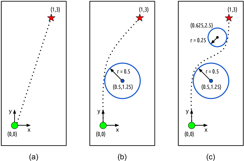
Figure 1: Illustration of the benchmark tasks (top view). Starting from the origin the robot should reach the goal (star mark). Circle obstacles (blue) are included to increase the problem complexity. (a) Go-to task, (b) one-obstacle task and (c) two-obstacles task. Position and size of the obstacles are expressed in meters.

III-B Problem components

The benchmark compares the performance of different configurations of the direct transcription method. Table I summarizes the variables evaluated in this study.

Regarding the complexity of the task, each path constraint added to (3) has to be verified at each node in (5), augmenting the size and density of the gradients required to find an optimal solution. This complexity is also increased when bounds on the state and control are considered. This is the case for the hardware experiments presented later in Section V-D. Here we measure the effect of including such bounds to the two-obstacle task, in a problem complexity labeled as ‘two-obstacle-bounds’.

At the same time, the performance also depends on the initial values of the decision variables of the NLP. Here we evaluate three different initialization methods, namely Zero, Linear and Incremental. In the first method all variables are naively set to zero before the optimization begins. The linear method initializes only the variables corresponding to the states of the robot, using a linear interpolation between the initial and desired final states. Finally, the incremental method uses the optimal solution of a simpler task (e.g. less constrained) as initial values for all variables.

TABLE I: Analyzed Components of a Direct Transcription Problem

Integration Scheme	Trapezoidal
	Hermite-Simpson
Problem Complexity	Go-to
	One-obstacle
	Two-obstacle
	Two-obstacle-bounds
NLP Initialization	Zero
	Linear interpolation
	Incremental
Number of Nodes
NLP Solvers	SNOPT
	IPOPT

III-C Performance criteria

The ultimate goal of TO is to obtain state and control trajectories that can be implemented on a real robot, such that a certain task is accomplished while an objective function is minimized. Accordingly, we measure the performance of the methods in terms of accuracy, solving time and quality of the solution.

Accuracy

The system dynamics are approximated using a piecewise polynomial function. A solution is only valid if such an approximation is accurate. In case of perfect accuracy, almost no stabilizing feedback control would be required during simulation. We measure the accuracy of the solution using the mean squared error between the planned and the actual total control trajectories measured when the complete system is simulated (i.e. an indication of the divergence between planned $(u^{*})$ and total $(u)$ control signals as defined in Section IV and represented in Fig. 2).

Running time

Ideally, the motion planner should be fast enough to compute trajectories online. However, depending on the configuration, different number of iterations might be required to solve the NLP. Here we use the total time required to find a feasible solution as indicator of performance. In contrast to the number of iterations, it provides an absolute value that can be used to compare among solutions obtained with different solvers and integration schemes.

Quality of the solution

The conditions of optimality for the continuous trajectory optimization problem are given by the Pontryagin’s minimum principle. In direct transcription such conditions are approximated by the Karush-Kuhn-Tucker (KKT) necessary conditions for the corresponding NLP (see e.g., [1]). Continuous and discrete conditions converge as $N\rightarrow\infty$ and $\Delta T\rightarrow 0$. In this paper the KKT conditions are satisfied by any given solution with a tolerance of $10^{-6}$. We compare the quality of the solutions in terms of optimality using the resulting value of the objective function.

IV Robot Model and Control Scheme

IV-A Robot model

The non-linear model of the ballbot dynamics is described in [13]. The robot is modeled as two rigid bodies, the torso of the robot and the ball. The two bodies are linked by three actuators. In our model, we neglect wheel dynamics and we assume that no slip or friction losses occur. The state vector of this ballbot is defined as

$$x=[\phi_{r}\quad\dot{\phi}_{r}\quad\phi_{p}\quad\dot{\phi}_{p}\quad\phi_{y}\quad\dot{\phi}_{y}\quad\theta_{x}\quad\dot{\theta}_{x}\quad\theta_{y}\quad\dot{\theta}_{y}]^{T},$$ (9)

where $\phi$ and $\dot{\phi}$ represent the torso angles and velocities in the roll, pitch and yaw directions $(rpy)$. Furthermore, the state includes the rotational angles of the ball $(\theta_{x},\theta_{y})$ as well as their derivatives $(\dot{\theta}_{x},\dot{\theta}_{y})$, representing the ball position with respect to the initial state. The control actions are defined by the wheels’ input torques $u=[\tau_{1}\,\tau_{2}\,\tau_{3}]^{T}$.

The desired goal state for all tasks is given by,

$$x_{g}=\left[0\quad 0\quad 0\quad 0\quad 0\quad 0\quad 8\quad 0\quad 24\quad 0\right]^{T}$$

where the goal angles of the ball ($\theta_{x}=8$ rad, $\theta_{y}=24$ rad) correspond to the desired spatial location ($x=1$ m , $y=3$ m), given that the radius of the ball is $r=0.125$ m.

IV-B Cost function, terminal conditions and total trajectory time constraint

A quadratic function is used for the intermediate cost, i.e.,

$$\psi(x_{k},u_{k})=x_{k}^{T}Qx_{k}+u_{k}^{T}Ru_{k}.$$ (10)

Where $\bar{x}_{N}=x_{N}-x_{g}$ is the difference between the last state of the trajectory $x_{N}$ and the desired goal state $x_{g}$. The diagonal cost matrices $Q,R$ weigh the contribution of the state and control to the total cost. Setting those values of $Q$ to zero that correspond to the rotational angles of the ball, tends to reduce the amount of time the robot is not in the upright pose, and at the same time use as little torque as possible along the path.

In direct transcription initial conditions are assumed to be fixed. Additionally, in the simulations and experiments presented in this paper, the desired goal state is added as a hard terminal condition to the NLP, (i.e., $x_{N}=x_{g}$). In case this condition is not satisfied the problem is considered infeasible. It is important to note that by using this hard constraint the use of a final cost function $\Psi(x_{N})$ can be avoided.

Finally, the time between nodes $(\Delta T)$ is chosen to be constant and included as a decision variable. A constraint is added bounding the total trajectory time $(T)$,

$$T_{min}\leq(N-1)\cdot\Delta T\leq T_{max},$$ (11)

where the bounds are given as a task specification. For this study we define that motions should be completed between $T_{min}=1.0$ s, and $T_{max}=3.5$ s.

IV-C Trajectory stabilization

Despite using an elaborated integration scheme or a very small discretization time, solutions obtained using direct transcription are based on an approximation of the system dynamics. Even in simulation very small numerical integration errors push the system towards instability. Therefore, it is necessary to stabilize the system.

In this work we use Time Variant Linear Quadratic Regulator - TVLQR (see e.g., [14]) to obtain a feedback controller. The derivation of this optimal controller is out of the scope of this paper. However, a descriptive explanation is provided for completeness: The dynamics of the system are linearized around the continuous optimal trajectory $\left(x^{*}_{t},u^{*}_{t}\right)$ using a Taylor approximation of (1). The state and control trajectory errors are defined as $\hat{x}_{t}=x^{*}_{t}-x_{t}$ and $\hat{u}_{t}=u^{*}_{t}-u_{t}$. Thus, its dynamics are described as a linear time varying system

$$\dot{\hat{x}}_{t}=A(t)\hat{x}_{t}+B(t)\hat{u}_{t}.$$ (12)

The state and input matrices are given by

$$A(t) = \left.\frac{\partial f\left(x,u\right)}{\partial x}\right\|_{x^{*}_{t},u^{*}_{t}}$$

$$B(t) = \left.\frac{\partial f\left(x,u\right)}{\partial u}\right\|_{x^{*}_{t},u^{*}_{t}}.$$

By solving the TVLQR problem for the system in (12), a matrix of time dependent optimal feedback gains $K(t)\in\mathbb{R}^{m\times n}$ is obtained. The resulting control scheme is illustrated in Fig. 2.

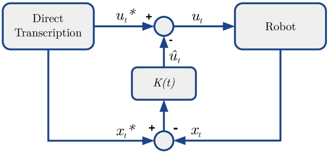
Figure 2: Complete control scheme. Feed forward control action is provided by the TO planner and a feedback stabilization control is computed using a time varying gain matrix, $K(t)$, obtained via TVLQR.

V Results

The results presented in this section were obtained using a standard laptop computer with 2.4Ghz Intel Core i5 (dual core) processor with 4GB 133Mhz DDR3 RAM. Feasibility tolerance of the NLP solvers was set to $1\times 10^{-6}$, meaning that all the constraints, including the terminal condition $(x_{N}=x_{g})$, are satisfied with an error bounded by this value.

V-A Optimal solution and stabilizer

Here we present the resulting state and control trajectories for the goto task obtained with a typical configuration: 100 Nodes, Hermite-Simpson integration scheme, linear initialization and SNOPT as NLP solver.

Fig. 3 presents the optimal trajectories for the states. The desired state is reached in $T=3.1$ s. Similarly, Fig. 4 shows the control trajectories and Fig. 5 shows the corresponding stabilizer gains obtained using TVLQR.

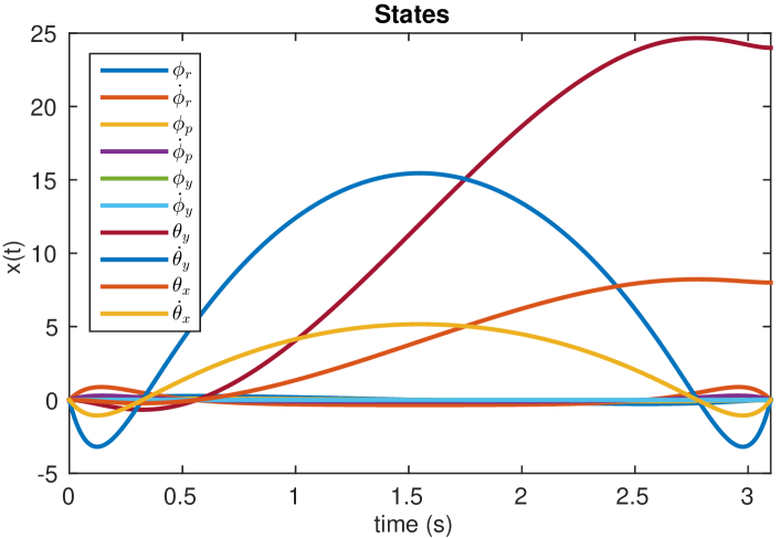
Figure 3: State trajectories for the goto task. Solution found using $N=100$ nodes, linear initialization, Hermite-Simpson integration and SNOPT solver. The optimal solution also includes the time increment between nodes $\Delta T=0.03131$ s. All velocities and body angles converge to zero.

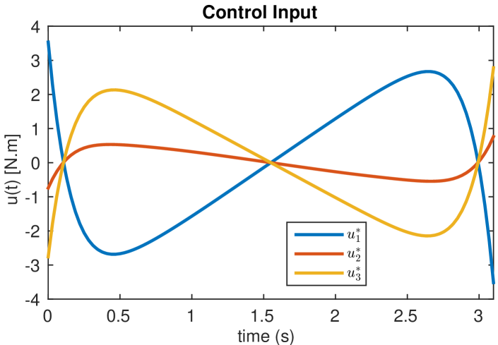
Figure 4: Control trajectories for the goto task. Solution found using $N=100$ nodes, linear initialization, Hermite-Simpson integration and SNOPT solver.

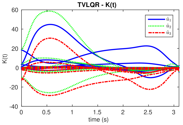
Figure 5: Feedback gains for stabilizing the goto task. Gains are grouped (line/color) by the corresponding control. Each feedback control $(\hat{u}_{i})$ is computed adding the weighted contribution of the state error ($\hat{x}$).

V-B Task complexity and initialization strategy

In this part, the performance of direct transcription for tasks of diverse complexity as well as the influence of different NLP initialization strategies are evaluated.

Firstly, we observed that the two-obstacles task cannot be solved using zero initialization regardless of the number of nodes, integration scheme or solver used. On the other hand, such a task can be solved using linear initialization. Fig. 6 shows the solving time required by the solvers to find a solution to the different tasks using the same scheme (100 nodes, trapezoidal interpolation and linear initialization). It can be seen that the complexity of the task affects the time required by the solvers. This is more significant in the case of SNOPT. Moreover, for the two-obstacle-bounds complexity, SNOPT does not find a feasible solution before reaching the maximum number of iterations ($1000$), irrespective of the integration scheme or number of nodes used.

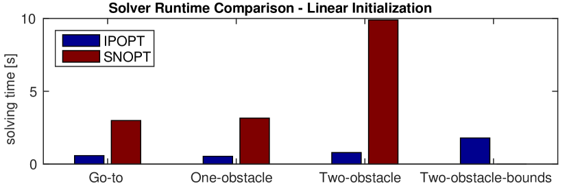
Figure 6: This plot compares the solving time for the different tasks and solvers using linear initialization method. Number of nodes $(N=100)$ and integration scheme (trapezoidal) are constant. SNOPT is not able to find a solution for the real robot task given those conditions.

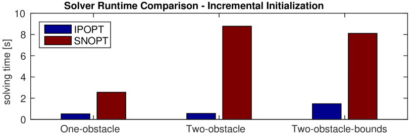
Figure 7: This plot compares the solving time for the different tasks and solvers using incremental initialization. Number of nodes $(N=100)$ and integration scheme (trapezoidal) are constant.

In Fig. 7 solving time for the different tasks and solvers are shown for the case of incremental initialization. Decision variables are initialized with the solution of the previous task. As expected in this type of initialization, the solving time is lower than those shown in Fig.6. Moreover, in this case SNOPT is able to find a solution for the two-obstacle-bounds complexity. Apart from the variation on running time and feasibility reported in this section, no significant differences were observed on the accuracy or quality of the solution given different initialization methods.

V-C Integration scheme

In this section we show the influence of the integration scheme and solvers in terms of run time, accuracy and quality of the solution. In order to obtain the corresponding data we use the one-obstacle task using zero initialization.

Fig. 8 compares the runtime for the integration schemes in combination with both solvers. While the absolute values of these measures are highly dependent on the CPU capacity, this section is concerned with their relative values. With a low number of nodes (i.e. $N<20$) both solvers show similar performance. However, with an increasing number of nodes the computational complexity of SNOPT is higher and increases faster than the one obtained with IPOPT. For both solvers, Hermite integration requires more CPU time than trapezoidal integration, but the difference is not significant.

Fig. 9 shows the divergence, in terms of mean squared error, between the planned and total control trajectories (during simulation). As it can be observed, the accuracy is independent of the solver. However, Hermite integration produces an error which is by several magnitudes lower than the one of trapezoidal integration.

Fig. 10 compares the value of the objective function after optimization. This value can be understood as being inversely proportional to the quality of the solution. The difference between the two solvers is marginal. However, Hermite integration is able to achieve a significantly lower objective function value, especially with a low number of nodes.

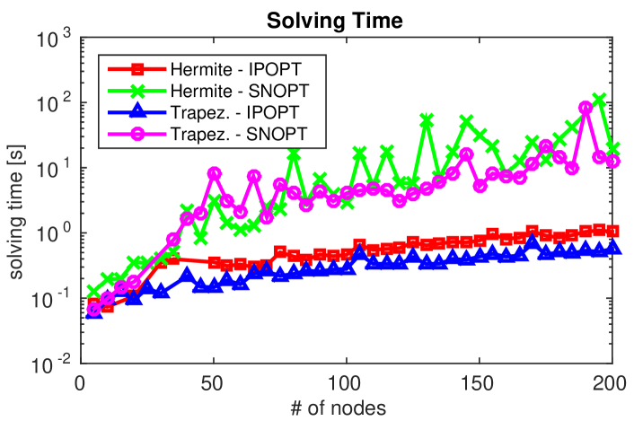
Figure 8: This plot shows the runtime of the different combinations of integration methods and solvers. For a low number of nodes, differences are small. However, with an increasing number of nodes, the runtimes of SNOPT are above those of IPOPT and also rise faster.

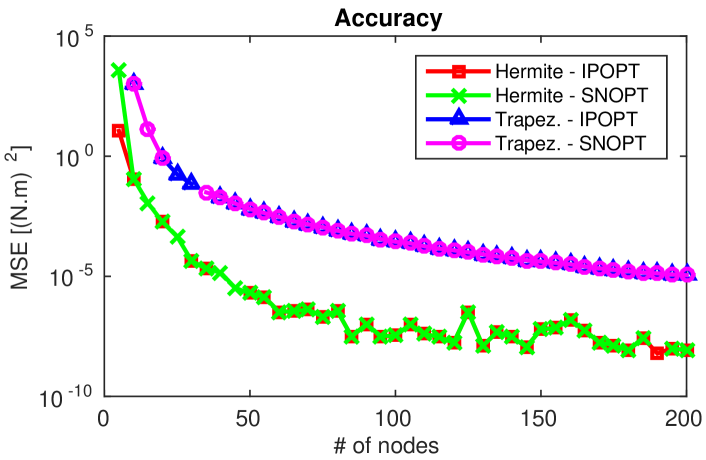
Figure 9: This plot shows the accuracy of the solution for both solvers and integration schemes. As indicator of accuracy we use the mean squared error (MSE) between the planned and the total control required to simulate the task. It can be seen that Hermite integration is significantly more accurate than trapezoidal integration.

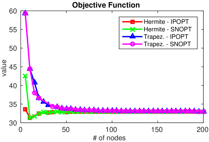
Figure 10: This plot shows the objective function value for the different combinations of integration methods and solvers. Especially for low number of nodes, Hermite integration clearly outperforms trapezoidal integration. For more than 50 nodes, the differences vanish.

V-D Hardware experiments

All the benchmark tasks shown in Fig. 1 (including those with path constraints) were applied to the real hardware in order to verify that these approaches also hold on a physical system. Control inputs and states were bounded to more conservative values avoiding aggressive behaviors and to operate in a safer regime. Moreover, upper bound for the total trajectory time was relaxed ($T_{max}=7$ s). Solutions were found using 100 Nodes, Hermite approximation and IPOPT as a solver. The robot used in the experiment is shown in Fig. 11 and a video with the experimental results can be found at https://www.youtube.com/watch?v=VGIROnFWgMw. In the video it can be seen that the robot executes the task synchronized with the simulation, following the planned trajectories.

Figure 11: Ball balancing robot. This robot consists of three major elements: the ball, the propulsion unit and the upper body (torso). The ball is driven by three omniwheels mounted on brushless motors with planetary gear heads. Through optical encoders on the motors, the ball rotation is measured providing onboard odometry for the robot.

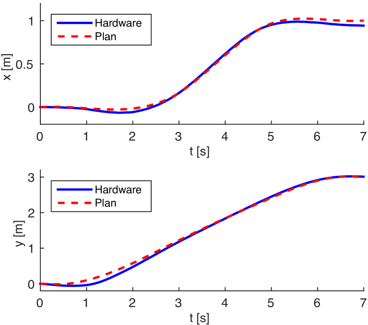
Figure 12: Position of the robot in $x$ and $y$ direction during execution of the two obstacles task. The blue solid line shows the measured data while the red dashed lie shows the planned trajectory. Solution time for this configuration is $1.79$ s.

The $xy$ position of the robot during execution of all tasks matches the planned trajectory fairly well with almost no deviation. Fig. 12 shows the results for the third task. Even though this is the most challenging task, it can be seen that the tracking behavior is very good. In summary, the hardware tests show good tracking performance, verifying that the optimized trajectory is dynamically feasible and that the tracking control is able to reject disturbances and model inaccuracies very well.

V-E Validation on a different robot

Results presented above are validated by applying the same methods on a simulated 3D quadrotor ($x\in\mathbb{R}^{12},u\in\mathbb{R}^{4}$) executing an obstacle avoidance task. Fig. 13 shows the trajectory followed by the quadrotor, starting from the origin and reaching the goal after avoiding a cylindrical obstacle. The complete motion can be seen in the supplemental video.

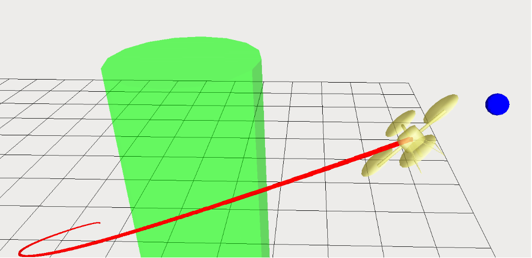
Figure 13: Quadrotor validation task. Blue dot represents the goal spatially located at $p=[5,5,5]$. A cylindrical obstacle ($r=1$) is centered at $x=2.5,y=2.5$.

We observed that the influences of the type of solver, dynamic constraints, initialization method and number of nodes are similar to the ones shown on the ballbot experiments. For instance, Table II shows the time required to solve this task for different configurations using zero initialization strategy. The same patterns can be observed: Solution time increases with the number of nodes and IPOPT is faster than SNOPT given the same integration scheme. As observed in Fig. 8, there is no clear pattern regarding solution times required by SNOPT when using different integration schemes. These results support the hypothesis that the conclusions drawn from the evaluation presented in this paper are not robot specific but that they can be extended to other platforms.

TABLE II: Verification Results - Solution Time (s)

N	IPOPT		SNOPT
	Hermite	Trapez.	Hermite	Trapez.
50	0.785	0.240	18.53	0.423
75	1.153	0.332	42.81	3.072

VI Analysis and Discussion

NLP solver

We observed that SNOPT requires more time in most of the comparisons. This is even clearer for the case of the two obstacle task, where the difference to IPOPT is significant. This can be explained by the need of SQP methods in finding a solution within a big active set of inequality constraints. As pointed out in other comparison studies [12], IPM tend to be faster in a NLP problem with many inequality constraints. Moreover, given a good initialization, the IPM algorithm always outperformed the SQP solver. In terms of quality and accuracy of the solution both solvers acted similarly under different schemes.

Integration scheme

The integration scheme has less influence on the solution time than the solver. However, selecting a Hermite-Simpson approximation has a considerable impact on the accuracy of the solution. As expected, the error decreases with the number of nodes, but this is not significant with respect to the better approximation reached with Hermite-Simpson. The quality of the solution is also affected by the integration scheme. Trapezoidal methods requires at least $50$ nodes to reach the same quality as the one obtained with Hermite integration using $20$ nodes. This fact, together with the running time results, where Hermite and trapezoidal schemes perform similarly when using IPOPT, suggests that Hermite integration scheme should be preferred.

Initialization

The aspect of initialization is closely related to the performance of the solver. We observed that direct transcription in general is considerably sensitive to the initialization strategy adopted at the NLP stage. Regardless of the solver, applying an adequate initialization policy clearly reduces the time to obtain a solution. This is a fundamental aspect for applying direct transcription online.

Hardware experiments

It has been shown that TO with a matching controller can be deployed on real hardware. The good match between simulated and real behavior can be observed both from the figures presented in this paper as well as from the video attachment overlaying simulated and physical robot. Small deviations between planned and real trajectories can be explained by model mismatches and sensor noise. These experiments validate the applicability of TO to real hardware and they are one of very few examples of using this technique on real underactuated robots.

Solving time

Ideally, the robot itself should be able to obtain plans online. Since the optimized trajectory is usually complemented with a stabilizing controller TO is not bound to run at the same rate or in hard real-time. However, the solving time of TO should be fast enough to react to large scale disturbances or unforeseen changes in the robot’s environment. The maximally acceptable solving time depends on the dynamics of the system and on the task. For the given example in Figure 7 the solving time is about 5 to 50 cycles of the inner stabilizing control loop. These solving times lie within a reasonable magnitude for online planning.

Failures during optimal trajectory search

TABLE III: Missing data points - configurations

Integration Scheme	Number of Nodes	Solver
Hermite	190	SNOPT
Hermite	15, 25, 40, 45	IPOPT
Trapez.	25,30	SNOPT

Occasionally the solver might not be able to find a solution, declaring numerical difficulties or because the maximum number of iterations has been reached. As observed in Fig. 8 and Fig. 10, data is missing for a few configurations of solver, integration scheme and number of nodes. Such configurations are reported in Table III. Further investigation is required to detect the fundamental reasons for these failures, as no clear pattern of the variables analyzed in this study is observed.

Finally, apart from the aforementioned cases, in Fig. 9 five other points are also missing. Such cases correspond to solutions for which the TVLQR method is not able to find a feedback controller and therefore the accuracy as defined in Section III-C cannot be determined. This is observed for some configurations with less than 30 nodes for both integration schemes and solvers. Further investigation regarding the relation between direct transcription and the solution of a TVLQR problem is required in order to identify the fundamental reason of such effect.

VII Conclusions

The comparisons performed in this work show clear patterns on the performance of direct transcription methods with respect to the different integration methods, solvers, initialization and problem types.

We showed a successful implementation of a direct transcription based motion planning and control approach for a real robot. For a problem of medium complexity, such as the one evaluated here, the solution convergences sufficiently fast so online planning using these methods comes in reach.

References

- [1] J. T. Betts, “Survey of numerical methods for trajectory optimization,” Journal of Guidance, Control, and Dynamics, vol. 21, no. 2, pp. 193–207, 1998.
- [2] J. Koenemann, A. Del Prete, Y. Tassa, E. Todorov, O. Stasse, M. Bennewitz, and N. Mansard, “Whole-body model-predictive control applied to the hrp-2 humanoid robot,” in IEEE-RSJ Int. Conference on Intelligent Robots and Systmes (IROS), 2015, pp. 3346–3351.
- [3] H. Dai, A. Valenzuela, and R. Tedrake, “Whole-body motion planning with centroidal dynamics and full kinematics,” in Humanoid Robots (Humanoids), 2014 14th IEEE-RAS International Conference on, 2014, pp. 295–302.
- [4] M. Posa, C. Cantu, and R. Tedrake, “A direct method for trajectory optimization of rigid bodies through contact,” International Journal of Robotics Research, vol. 33, no. 1, pp. 69–81, 2014.
- [5] G. Schultz and K. Mombaur, “Modeling and optimal control of human-like running,” Mechatronics, IEEE/ASME Transactions on, vol. 15, no. 5, pp. 783–792, 2010.
- [6] C. Hargraves and S. Paris, “Direct trajectory optimization using nonlinear programming and collocation,” Journal of Guidance, Control, and Dynamics, vol. 10, no. 4, pp. 338–342, 1987.
- [7] O. von Stryk and R. Bulirsch, “Direct and indirect methods for trajectory optimization,” Annals of Operations Research, vol. 37, no. 1, pp. 357–373, 1992.
- [8] V. Becerra, “Solving complex optimal control problems at no cost with psopt,” in Computer-Aided Control System Design (CACSD), 2010 IEEE International Symposium on, 2010, pp. 1391–1396.
- [9] P. Gill, W. Murray, and M. Saunders, “SNOPT: An SQP algorithm for large-scale constrained optimization,” SIAM Review, vol. 47, no. 1, pp. 99–131, 2005.
- [10] A. Wachter and L. T. Biegler, “On the implementation of a primal-dual interior point filter line search algorithm for large-scale nonlinear programming,” Mathematical Programming, vol. 106, no. 1, pp. 25–57, 2006.
- [11] B. Conway, “A survey of methods available for the numerical optimization of continuous dynamic systems,” Journal of Optimization Theory and Applications, vol. 152, no. 2, pp. 271–306, 2012.
- [12] J. T. Betts and J. M. Gablonsky, “A comparison of interior point and SQP methods on optimal control problems,” March 2002, tech. report.
- [13] P. Fankhauser and C. Gwerder, “Modeling and control of a ballbot,” Bachelor thesis, ETH - Zurich, 2010.
- [14] R. Tedrake, “Underactuated robotics: Algorithms for walking, running, swimming, flying, and manipulation (course notes for mit 6.832),” Downloaded in Fall, 2014. [Online]. Available: http://people.csail.mit.edu/russt/underactuated/